Carbon Footprint A Case Study on the Municipality of Haninge - Ho
←
→
Page content transcription
If your browser does not render page correctly, please read the page content below
Ho

                             Carbon Footprint
A Case Study on the Municipality of Haninge

                                               WEILING WU

             Master of Science Thesis in Technology and Health

                                              Stockholm 2011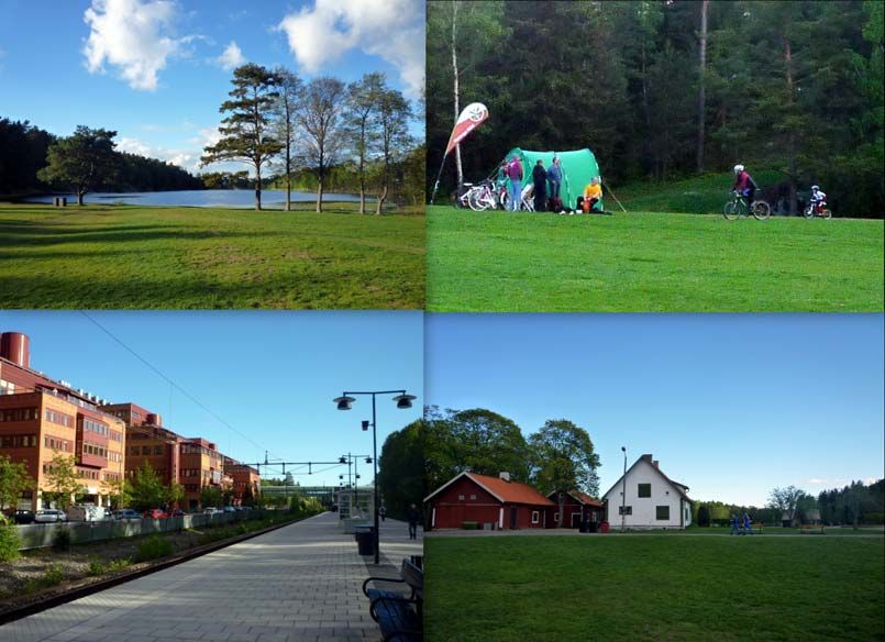
ii
Carbon Footprint

-- A Case Study on the Municipality of Haninge

                                           Weiling Wu

          Master of Science Thesis in Technology and Heath

                             Advanced level (second cycle)

                               Supervisor: Elisabeth Ilskog

                            Examiner: Eva-Lotta Thunqvist

                     KTH, School of Technology and Health

                                       TRITA-CHB 2011:5

                             Royal Institute of Technology

                                                  KTH STH

                                          Marinens väg 30

                               SE-136 40 Handen, Sweden

                                    http://www.kth.se/sth
                                                              iii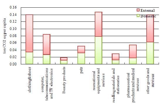
iv
Carbon Footprint – a Case Study on the Municipality of Haninge
                              Weiling Wu

KTH, Uppsala University, and Swedish University of Agricultural Sciences

                             Supervised by

                            Elisabeth Ilskog

                 KTH, School of Technology and Health

                    Submitted in Partial Fulfilment of

              Master of Science in Sustainable Development

                    Faculty of Technology and Science

                           Uppsala University

                              Spring 2011

                                                                           v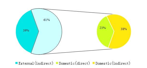
vi
Abstract

Carbon Footprints, as an indicator of climate performance, help identify major GHG emission
sources and potential areas of improvement. In the context of greatly expanding sub-national
climate efforts, research on Carbon Footprint accounting at municipality level is timely and
necessary to facilitate the establishment of local climate strategies. This study aims at
exploring the methodologies for Carbon Footprint assessment at municipality level, based on
the case study of Haninge municipality in Sweden. In the study, a Greenhouse Gas inventory
of Haninge is developed and it is discussed how the municipality can reduce its Carbon
Footprint. The Carbon Footprint of Haninge is estimated to be more than 338,225 tonnes CO2
eq, and 4.5 tonnes CO2 eq per capita. These numbers are twice as large as the production-
based emissions, which are estimated to be 169,024 tonnes CO2 eq in total, and approximately
2.3 tonnes CO2 eq per capita. Among them the most important parts are emissions caused by
energy use, and indirect emissions caused by local private consumption. It is worth noting that
a large proportion of emissions occur outside Haninge as a result of local consumption.
Intensive use of biomass for heat production and electricity from renewable sources and
nuclear power have significantly reduced the climate impact of Haninge. The major barrier
for Carbon Footprint accounting at municipality level is lack of local statistics. In the case of
Sweden, several databases providing emission statistics are used in the research, including
KRE, RUS, NIR and Environmental Account.

Key words: Carbon Footprint, Greenhouse Gas emissions, inventory, municipality, Haninge.

                                                                                               vii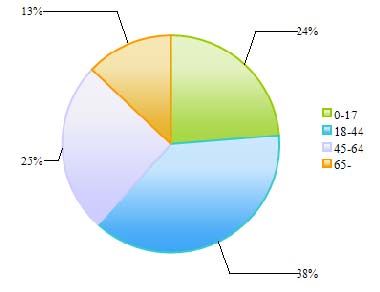
viii
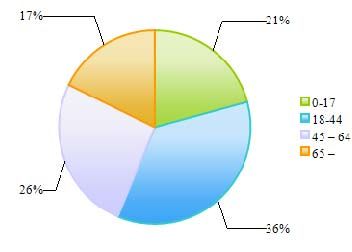
Table of Content
Abbreviation ............................................................................................................................. 1
1. Introduction .......................................................................................................................... 2
1.1. Definition of Carbon Footprint .................................................................................... 2
1.2. Previous studies on Carbon Footprint .......................................................................... 4
1.3. Haninge Municipality .................................................................................................. 5
1.4. Aim .............................................................................................................................. 7
2. Methodology for Carbon Footprint accounting ................................................................ 8
2.1. GHG accounting based on production or consumption ............................................... 8
2.2. Methodologies of Carbon Footprint calculation ........................................................ 10
2.2.1. Environmentally Extended Input-Output Analysis ......................................... 11
2.2.2. Process Analysis ---Life Cycle Assessment (PA- LCA) ................................. 12
2.2.3. Hybrid Approaches .......................................................................................... 12
2.3. Standardization .......................................................................................................... 13
2.4. Research methodology applied in this thesis ............................................................. 15
3. Results and analysis: Carbon Footprint of Haninge ...................................................... 17
3.1. Greenhouse Gas inventory of Haninge ...................................................................... 17
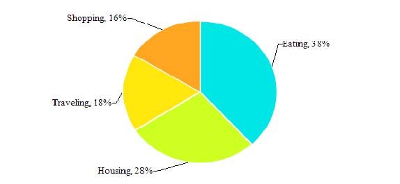
3.2. Swedish private consumption based GHG inventory ................................................ 22
3.2.1. Eating ............................................................................................................... 26
3.2.2. Housing ............................................................................................................ 27
3.2.3. Travelling......................................................................................................... 28
3.2.4. Shopping .......................................................................................................... 29
3.3. Climatic impact of Haninge and comparison with national data ............................... 30
3.4. Analysis of influential factors on the Carbon Footprint of Haninge ......................... 31
3.4.1. Population and population density .................................................................. 31
3.4.2. Income level .................................................................................................... 333.4.3. Transport pattern.............................................................................................. 33
4. Discussion ............................................................................................................................ 34
4.1. Reducing climatic impact of the energy sector in Haninge ....................................... 34
4.2. Refining local climate strategies ................................................................................ 35
4.3. Reducing the Carbon Footprint of private consumption of Haninge ......................... 36
4.4. Establishing a regular statistical collection procedure for long-term monitoring...... 37
4.5. Methodology of Carbon Footprint assessment at municipal scale ............................ 38
4.6. Limitations and further study ..................................................................................... 39
5. Conclusions ......................................................................................................................... 39
6. Acknowledgements ............................................................................................................. 41
References ............................................................................................................................... 42
Appendix ................................................................................................................................. 44
Appendix I Description of GHG accounting standards ................................................... 44
Appendix II Tables of energy balance of Haninge (Year 2008) ...................................... 48
Appendix III Instruction of product groups in Table 3.3 ................................................. 49
Appendix IV Example of GHG accounting Excel sheet for Haninge ............................. 51
xAbbreviation
CF ------ Carbon Footprint
GHG ------ Greenhouse Gas
IPCC ------ Inter-governmental Panel of Climate Change
SEPA ------ Swedish Environmental Protection Agency
ICLEI ------ Local Governments for Sustainability
NIR ------ National Inventory Report
WRI ------ World Resource Institute
WBCSD ------ World Business Council for Sustainable Development
IEAP ------ International Local Government GHG Emissions Analysis Protocol
GHG Protocol ------ The Greenhouse Gas Protocol, a corporate accounting and reporting
standard.
PAS 2050 ------ PAS2050 2050: 2008 Specification for the assessment of the life cycle
greenhouse gas emissions of goods and services
SEI ------ Stockholm Environment Institution
KRE ------ Municipal and regional energy statistics / Kommunal och regional energistatistik
(in Swedish)
RUS ------ Regional Development and Co-operation in environmental system / Regional
Utveckling och Samverkan i miljömålssystemet
SMED ------ Swedish Environmental Emissions Data / Svenska MiljöEmissions Data (in
Swedish)
BSI ------ British Standards Institution
LULUCF ------ Land use and land use change
11. Introduction
With growing concern over climate change globally, emission control of Greenhouse Gases
(GHGs) has been put on the agenda of both developed and developing countries. Despite the
great difficulty in achieving sufficient agreement in international climate negotiation, cities
have realized that they can actually proceed faster than the international climate negotiation
with more flexible ways of corporation. Actions are taken at sub-national levels to mitigate
climate change. At COP 16 in Cancún, local governments were for the first time recognized
as key governmental stakeholders in climate change efforts (ICLEI, 2010a). As a key
component of the Mexico City Pact which is signed by 138 cities around the world, the
Carbonn Cities Climate Registry has been launched as an official reporting mechanism for
cities to register their GHG reduction commitment (ICLEI, 2010b). As the initial step of
action, GHG accounting supports policy making process since it gives an overall picture of
the city's emission situation, helps identify major emission sources and potential areas of
improvement. It is also an essential tool to assess the performance of local climate actions,
and to support improvement of policies. To ensure local climate action is "measurable,
reportable, and verifiable", feasible ways of assessing local GHGs emissions are called for.
Hence research on assessment of local Carbon Footprint is timely and necessary in assisting
assist the expanding sub-national climate efforts.
This thesis explores the methodology and feasibility of municipal Carbon Footprint (CF)
accounting, and its implications on local climate efforts. A case study of Haninge in Sweden
is conducted. The report constitutes five chapters: chapter 1 gives a overall picture of the
study as well as background information of CF; in chapter 2 different methodologies are
discussed and compared, accordingly approaches applied in this research are selected and
described; in chapter 3 Greenhouse Gas emission inventories of Haninge from both
production and consumption perspectives are presented and analyzed; the last two chapters
present discussion of results and conclusions. The research was undertaken at the Kungliga
Tekniska Högskolan (KTH) as a thesis for the master’s programme in Sustainable
Development in Uppsala University.
1.1. Definition of Carbon Footprint
There is no exact academic definition of Carbon Footprint yet, and debate continues
(Wiedmann & Minx, 2008). The concept of Carbon Footprint derives from the concept of
Ecological Footprint raised by Wackernagel and Rees in 1996. As one part of Ecological
Footprint, the land area needed to sequester CO2 emitted from burning fossil fuel is measured
to estimate the land requirement for energy use (Wackernagel & Rees, 1996). However, with
increasing public and political concern of climate change, Carbon Footprint has been
developed into a separate concept with extended scopes.
Although no common definition has been provided by the academic world, there are many
definitions in wider literature. As can be seen from the summary of "Carbon Footprint"
2definitions from the grey literature by Wiedmann and Minx (2008), several key elements that
formulate a valid CF concept have not been agreed on: Should the calculation include carbon
dioxide exclusively or other GHGs as well? Should it be measured in CO2 equivalent or
hectares as in Ecological Footprints? Should the indirect emission be considered? How can
the temporal as well as spatial boundaries be set?
The definition proposed by Wiedmann answers some of these questions: "The carbon
footprint is a measure of the exclusive total amount of carbon dioxide emissions that is
directly and indirectly caused by an activity or is accumulated over the life stages of a
product." (Wiedmann & Minx, 2008, p.4) Though there are difficulties regarding
methodology, the author holds that indirect emissions should also be included in CF
inventories. It has been demonstrated by some case studies that indirect emissions constitute
the majority of Carbon Footprint of a functional unit (Larsen & Hertwich, 2009a). Exclusion
of indirect emissions arising from the upstream supply chain as well as downstream disposal
is very likely to bring about considerable underestimation. Furthermore, in the context of
ethics and equity, inclusion of indirect emissions includes the environmental impact of
manufacturing nations into the account of consuming nations, therefore avoiding an unfair
shift of responsibility from rich countries to developing countries in the globalizing economy.
Inclusion of indirect emissions is in accordance with the definition used in a case study of
York neighborhoods, where Carbon Footprint is defined as the total amount of CO2 emissions
which result directly and indirectly from the individual use of goods and services, covering
both individuals’ immediate emissions and emissions arising during the production process
(Haq & Owen, 2009).
An open definition that attempts to allow for applications at varied scales is provided by
Peters (2010, p.245): "The ‘carbon footprint’ of a functional unit is the climate impact under a
specified metric that considers all relevant emission sources, sinks, and storage in both
consumption and production within the specified spatial and temporal system boundary." This
definition offers large flexibility on both objects and emission categories of interest. It also
covers the main stages of the carbon cycle related to anthropogenic activities. The
disadvantage is that this definition is too broad to help set research boundaries for a specific
case study.
Given the need of a well-defined scope for the study, the following definition of Carbon
Footprint is applied here: “Carbon footprint is the life-cycle GHG emissions caused by the
production of goods and services consumed by a geographically-defined population or activity,
independent of whether the GHG emissions occur inside or outside the geographical borders
of the population or activity of interest.” (Larsen & Hertwich, 2009a, p.792) According to this
definition, CF refers to GHG emissions based on the consumption of a defined population,
therefore calculation of the CF of a city or municipality should not be limited to its
geopolitical boundaries.
31.2. Previous studies on Carbon Footprint
Research on Carbon Footprint are conducted at various scales from national to municipal
levels, from industries to certain kind of products. As this study focuses on municipal climate
impact, this literature review includes only studies on national and municipal Carbon
Footprints. Nevertheless, one should bear in mind that efforts at carbon accounting are also
common in private and industrial sectors as a result of widespread climate concern.
Besides governmental reporting mechanisms under the UNFCCC system academia also
shows great interests in exploring the underlying rules of dynamic Carbon Footprints. A
cross-country analysis of the CF of consumption using a multi-regional input-output (MRIO)
model based on Global Trade Analysis (GTAP) database (Hertwich & Peters, 2009) shows
that per capita CF increases as countries become wealthier. Meanwhile, consumption pattern
changes with rising income: food is of more importance in the expenditure of low-income
countries. The study also concluded that indirect impact in the supply chain is more important
than direct impact: shelter, food and mobility are the most important consumption categories.
Furthermore, as developed countries are shifting their carbon-intensive industries to less
developed countries, an increasing proportion of indirect emissions tend to occur outside the
borders of consumption countries. The significant impact of importing in developed countries
has been demonstrated by some studies. In UK, over half of the average households' Carbon
Footprint comes from embedded CO2, of which 40 % took place outside UK in 2004. The
proportion has been continuously rising since 1990 (Druckman & Jackson, 2009). In general,
it has been widely accepted that income level and international trade play important roles in
the country's CF status.
There is an increasing trend towards applying consumption-based inventories to municipal
Carbon Footprint accounting instead of the traditional production-based method, as it has
been widely accepted that indirect emissions actually dominate local emission categories
especially in cities of developed countries. A case study of a Norwegian city indicates that
approximately 93% of the CF of municipal services is indirect emissions from upstream
procedures, "underlying the need of introducing consumption-based indicators that take into
account upstream GHG emissions" (Larsen & Hertwich, 2009, p.791). In the same year, 30%
of total US household CO2 emssions occurred outside the US as a result of growing
international trade, with household income and expenditure recognized as the best predictor of
both domestic and international portions of total CO2 impact (Weber & Matthews, 2007). In
light of the fact that indirect emissions are becoming increasingly important, a shift of
research interest from a production perspective to consumption perspective is observed.
Carbon Footprint accounting is applied as a useful tool to help municipalities develop local
climate strategies. For example, SEI conducted Carbon Footprint analysis for the
neighborhoods of York and the surrounding area in the UK (Haq & Owen, 2009). With an
average CF of 12.58 tonnes of CO2 per capita per year, housing and transport accounted for
nearly 60% of the total emissions and were identified to be the key sectors to work on.
Analysis of CF together with other factors such as ‘green’ attitudes and local infrastructure
over different districts of York also helps select the pilot neighborhood for promoting green
4lifestyle. At a larger scale, Carbon Footprint assessment is used as an indicator of community
planning. A comparison of the CF of 429 Norwegian municipalities (Larsen & Hertwich,
2009b) shows that CF changes significantly with size and wealth. 500,000 inhabitants is
recognized as a possible size of municipality to achieve the optimal municipal CF. It is
explained that up to a certain size, the efficiency of provision of public service increases with
population density. On the other hand, larger municipalities could encounter other social
problems which require additional public service.
While policy makers and practitioners are striving for improved local GHG inventories to
support climate mitigation strategies, academia has started to take the challenge of developing
and implementing calculation tools for embedded municipal Carbon Footprint. Hogne and
colleagues developed a specific consumption-based municipal GHG inventory based on
environmentally input-output analysis (EEIOA), which has been implemented in several
Norwegian municipalities (Hogne et al., 2010). REAP is another tool developed by SEI
which allows consumers to calculate the full supply chain emissions as a result of individual
consumption simply by putting in expenditure data on different product categories (Paul et al.,
2010). This tool is being developed for the UK and Sweden with country-specific databases.
Despite of the importance of CF accounting for enhancing municipal climate performance,
applying Carbon Footprint calculation and analysis on municipality level is uncommon in
academic research.
1.3. Haninge Municipality
Located at southern suburban Stockholm, Haninge is a small-sized city covering 2,190 km2,
with 454 km2 land and 1,736 km2 water (Haninge Municipality, 2010a). Haninge consists of
both urban districts and suburban areas (see map of Haninge, Figure 1.1).
With its 75,071 inhabitants (in 2009), Haninge ranks 25th in size among Sweden's
municipalities. The population structure is relatively young with an average age of 38. The
municipality is growing at the expected rate of 1000 persons per year, which implies a
population of 100,000 in 2030. Most of the population (50,000) live in the seven city districts.
Among the 31,100 dwellings of Haninge, 18,870 are apartments and 12,230 are houses
(Haninge Kommun, 2010a).
The small business sector dominates the city's economy and 95% out of the over 4,600
registered businesses have fewer than five employees. The main industries are logistics, car,
construction and real estate. Major companies include Coca Cola AB, Recipharm, AVL /
MTC, Tech Data, Frigo Scandia, Kemetyl, logistics enterprises such as Prologis, Green Cargo
and Lagena. 77% of the municipality's population aged between 20 and 64 are employed,
among which 30% work within the city and 47% commute out of Haninge. Meanwhile
10,300 workers commute in from other parts of the county (Haninge Kommun, 2010a).
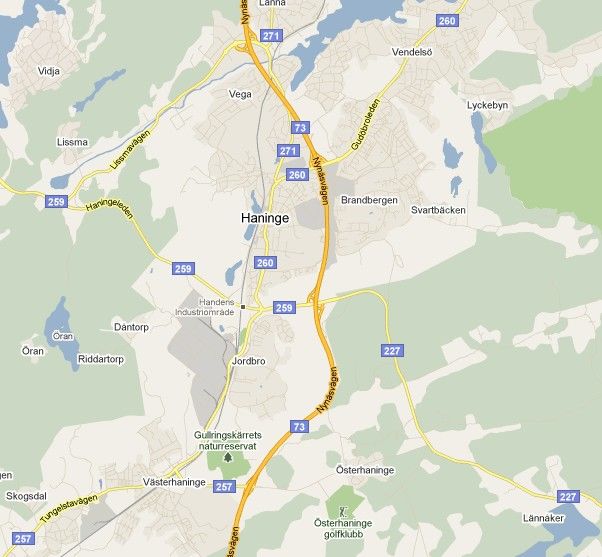
5Figure 1.1 Map of Haninge
Source: Google map.
As a typical small city in Sweden, there are few carbon-intensive industries within Haninge.
The only significant emission source registered on the 1 Swedish Pollution Release and
Transfer Register system1 is the district heating plant in Jordbro district. As is shown in
Figure 1.2, heat for the area is supplied by the district heating plant and waste generated by
activities in Haninge are delivered to a waste treating site in Sofielunds outside Haninge.
Sewage is also sent to Henriksdal sewage treatment plant outside Haninge.
1
http://utslappisiffror.naturvardsverket.se/
6Concerned about climatic issues, the municipality has developed its own climate strategy. The
overall objective to reduce Greenhouse Gas emissions by 90% in 2050 compared with 1990
while in the short term a 40% reduction by 2020 is expected. (Haninge Kommun, 2010b)
Figure 1.2 Map of Haninge, with Jordbro district heating plant (yellow tag) and Sofielunds
landfill (green tag) marked.
Source: Swedish Pollution Release and Transfer Register system
1.4. Aim
The hypothesis of the study is that it is possible to calculate Carbon Footprint of a relatively
small municipality with available data. The overall expectation is that the results can be
communicated to the public sufficiently, and specific climate strategies aiming at local
improvements can be established accordingly. Therefore the aim of the study is to identify a
method for assessing Carbon Footprint at municipal level and to explore how municipalities,
through relevant planning activities, can reduce their Carbon Footprint. To place this in a
concrete context the research will be based on a case study of Haninge municipality.
72. Methodology for Carbon Footprint accounting
2.1. GHG accounting based on production or consumption
Regarding Greenhouse Gas emissions for nations and cities, there are two different ways of
accounting: one from the perspective of production and, the other from the perspective of
consumption. Depending on choice of perspective, different results and policy implication
will be obtained.
The traditional production-based inventories estimate GHGs emissions from local production
processes within a geographically defined area, regardless where the output is consumed
(Larsen & Hertwich, 2009a). In this case, both upstream and downstream processes outside
the municipal borders are excluded, while production for exports is included. A production-
based inventory can be developed either by top-down method (allocate national emissions to
the defined area) or bottom-up modeling (gathering local emission data) (Larsen & Hertwich,
2009a). Calculation of GHG emissions from a production perspective has been widely applied
at national scale. For example, the IPCC guidelines are designed to help nations develop their
GHG inventories from the production perspective with the results reported to UNFCCC.
The recently emerging consumption-based inventories allocate all upstream GHG emissions
from the production and delivery processes to the final consumer, namely a defined
population (nation, city or municipality) (Larsen & Hertwich, 2009a). In contrast to
production-based accounting, consumption-based accounting includes allopatric emissions
caused by local consumption while excludes the emissions from local production of exported
goods. Unlike production-based inventories, no strict geographical borders are set for
consumption-based methods. A number of tools have been developed for a consumption-
based inventory, including Input- Output Analysis (IOA), Life Cycle Assessment (LCA), and
the hybrid IO-LCA method.
The relation between production-based and consumption-based inventories can be expressed
by Figure 2.1. In an open economy, the difference between the two is derived from import and
export. In a closed economy where neither import nor export is involved, the two inventories
could have completely overlapped with each other. At the global scale, what is produced is
also consumed on the planet as a whole. The difference between a production perspective and
consumption perspective is important only when the targeted entity has a considerable amount
of import and export. With the progress of globalization, there is a trend that consumption-
based emissions increasingly deviate from production-based emissions for nations and cities,
as what is produced is often exported and consumed in other areas. Thus it is interesting to
look at the difference between the two types of GHG inventories and the methods generate
different messages for policy making.
8Consumption‐based account
Production‐based account
Emissions from import Emissions from export
Common area: emissions from products / services both
produced and consumed domestically
Figure 2.1 GHG emissions from production perspective and consumption perspective
Applying a production-based accounting usually aims at actions reducing GHGs emissions
within geographical borders (Larsen & Hertwich, 2009a), while consumption-based
accounting mainly aims at influencing emissions through out the supply chains by improving
consumer behaviour. To choose a proper accounting method one should clarify the practical
objective of the study. For example, to explore the potential of emission reduction for a
manufacturing city whose economy is mainly built on export and where production dominates
consumption, production-based inventories are more likely to help identify the main sections
for improvement. On the other hand, as is the case of most small-sized municipalities in
developed countries, local consumption relies heavily on imports from all over the world.
This is not a rare situation. A number of studies have identified consumption, especially in the
industrialized world, as the main driver of environmental pressure (Larsen & Hertwich,
2009a). Consumption-based accounting is thus called for to break through geographical
boundaries and conduct a comprehensive estimation on the climate impact of a defined
consumer group. An important target of consumption-based accounting is to identify large
emitting sectors in the consumption category and explore improvement in consumer
behaviour. However, when looking at the consumption-based analysis, one should keep in
mind the drawbacks of this method: firstly, there are great uncertainties in statistics for
upstream emissions of imported products due to diverse manufacturing parameters in different
nations such as technology, transport, environmental regulations; secondly, there is a risk that
policy instruments based on the consumption perspective may be poorly aimed as the nation
itself does not have control over the upstream procedures that occur in other countries.
Most industrialized countries are allocated greater emissions from a consumption perspective
compared with a production perspective (Swedish Environmental Protection Agency, 2010).
In the case of Sweden, the total production-based emissions were 76 megatonnes CO2
equivalent in 2003, while the consumption-based emissions were 95 megatonnes CO2
9equivalent (Swedish Environmental Protection Agency, 2010). This means that 25% of GHG
emissions from domestic consumption occur in other parts of the world. As a typical small-
sized city in the industrialized world, Haninge’s consumption sector is of larger importance
than production and the city relies heavily on imports. Therefore, it is appropriate to look at
the consumption-based inventory, i.e. Carbon Footprint, to identify the global climate impact
of the municipality's consumption. GHG accounting from both consumption and production
perspectives will be conducted however in the interests of comparison. Based on this premise,
currently available methodologies and standards for developing a consumption-based
accounting (CF) are further discussed in the following section.
2.2. Methodologies of Carbon Footprint calculation
Due to the many scales of analysis (global, national, city/county, product), there is no single
standard methodology for consumption-based Carbon Footprint analysis. However, three
main methodologies are now under development for cases at varied scales, including
Environmental Expanded Input-Output (EEIO) analysis, Life Cycle Assessment (LCA), and
Hybrid IO-LCA methods (Wiedmann, 2009). Choice of method depends on functional unit
and scale. As illustrated by Figure 2.2, Input-Output models are commonly applied to CF
calculation at global and national level, hybrid models are applicable at sub-national scale,
organizations or industrial sectors, while Process-based LCA dominates the CF assessment of
products and services.
Figure 2.2 Carbon Footprint methods on different scales of application
Source: (Peters, 2010)
Processed-based LCA provides a comprehensive accounting product CF over its whole life
cycle. However, the LCA method requires comprehensive and specific data for each product.
It is therefore too data-demanding for studies on an entire entity such as an organization, a
city, or a nation, whose operation involves various products and services. EEIO analysis, with
less demand on specific data, is widely applied at national scale (Minx et al, 2009). The
hybrid IO-LCA method, combining the advantages of both EEIO and LCA methods, is newly
proposed and is being increasingly used in practice (Peters, 2010). The sector with the most
10potential for application of hybrid method is believed to be sub-national cases such as CF
analysis of cities, countries or organizations.
2.2.1. Environmentally Extended Input-Output Analysis
Principally formulated by Wassily Leontief in the 1930s, economic input-output analysis
(EIOA) is an economic modelling technique disclosing the interaction between sectors,
producers and consumers (Wiedmann, 2009). This economic tool was later (1970s) extended
to cover the generation and elimination of pollution, which were integrated into the economic
process (Leontief, 1970). This Environmentally Extended Input-Output (EEIO) analysis
provided an alternative approach for calculating Carbon Footprint when the concept came up
in 1990s. The IO methodology is based on supply and use tables describing the product flows
through the economy. In EEIO analysis, related emissions are linked to the input-output tables,
making it possible to see the direct emissions caused by an entity's production and the indirect
emissions of its suppliers (Swedish Environmental Protection Agency, 2010).
Since the IO analysis is based on cash flow, emissions are linked to cash flows. For each unit
of money spent on a product sector, there is a related emission. Therefore it is possible to
calculate consumption-based emissions through EEIO analysis. Once an Input-Output table is
established for an economy, a cost-efficient and consistent analysis of CFs can be conducted.
The acceptance of EEIO as a method of Carbon Footprinting varies across different scales of
application. EEIO analysis dominates calculation for national CF (Minx et al., 2009), as it can
analyze the complex system with many sectors and material flows in a resource-efficient way.
At organizational level, IO analysis is also considered an optional methodology for
accounting an entity's upstream emissions through linking IO models with the financial
accounts (Minx et al., 2009). Despite of increasing demand of CF information for
municipalities and cities in support of policy making process, CF accounting for small spatial
areas are still at its infancy stage, and application of EEIO method at this scale remains
largely unexplored (Minx et al., 2009). One potential application is that the well-established
national inventory can be combined with local expenditure or population data to get a general
estimation of local Carbon Footprint, when the specific data available is not sufficient to
conduct a local IO analysis. It can be useful considering the fact that many cities and
municipalities do not have a comprehensive record of economic activities and related
emissions.
Despite its wide-ranging application in CF, barriers exist for IOA’s application in certain
areas. One of the disadvantages is that IOA requires specialist knowledge in economic and
environmental theory and frameworks (Wiedmann, 2009) in which many practitioners in
corporations and municipalities are lacking. More importantly, it is often argued that the
aggregation uncertainty in IOA may lead to less accurate results then Process Analysis
(Wiedmann, 2009). Therefore, a holistic approach such as hybrid approach is needed to
reduce the uncertainty.
112.2.2. Process Analysis ---Life Cycle Assessment (PA- LCA)
LCA based on Process Analysis is a bottom-up approach developed for a holistic assessment
of the environmental impacts of individual products from cradle to grave. As its definition
usually includes non-carbon Greenhouse Gas emissions and uses CO2 equivalent as the unit of
measurement, Carbon Footprint is very similar to the Global Warming Potential (GWP)
indicator in LCA (Weidema et al., 2008). Thus LCA can be used to estimate the CF of
products throughout their life cycle. It is an efficient method to obtain a comprehensive CF
for certain products, for which LCA databases have been well established. As a dominant
method for product CF assessment, some LCA standards have been developed to standardize
data collection and calculation processes, including ISO 14040 and PAS 2050. The
standardization makes it possible to compare the CF of similar products, and to provide the
foundation for CF labelling.
However, when applying LCA to Carbon Footprinting, one might suffer from a system
boundary problem, which is a major difficulty for LCA. Especially for open-loop systems
with recycling and reuse processes, designating system boundaries requires practitioners to
have profound knowledge in LCA. A systematic truncation error is likely to occur when
system boundaries are defined arbitrarily, causing relevant emissions to be ignored. The other
limitation is that LCA is not appropriate for estimating CF of larger entities such as
municipalities, cities or industrial sectors, because it demands a huge amount of data on the
products and intensive work on information processing. Even though estimates can be derived
using information available in LCA databases, results will become increasingly patchy as a
subset of individual products is assumed to be representative for a larger product group and
information from different databases have to be used, which are usually not consistent
(Wiedmann & Minx, 2008).
2.2.3. Hybrid Approaches
Hybrid approaches integrate IOA and Process Analysis, using both sectorial and process-
specific data. The first hybrid approach combining IOA and Process Analysis was introduced
by Bullard in 1978 (Bullard et al., 1978), aiming to calculate the energy cost of goods or
services with a certain degree of accuracy. In a hybrid analysis of target products, IOA can be
used to determine the total energy cost of input materials which are typical products of IO
sectors, and further Process Analysis is only demanded for input materials that are atypical in
IO sectors (Bullard et al., 1978). With the development of research on Carbon Footprinting,
hybrid approaches are increasingly applied by researchers within the field. Berners-Lee and
colleagues (2010) created a hybrid model of GHG accounting for small and medium sized
businesses, where both national Input-Output data and PA-LCA techniques are applied.
Hybrid approaches can be divided into three categories: firstly, tiered hybrid analysis, in
which the direct and downstream processes and important lower order upstream procedures of
a product are examined in detailed Process Analysis, while the remaining parts are covered
with IOA; secondly, Input-Output based hybrid analysis, in which important Input-Output
12sectors are further disaggregated if more detailed sectoral monetary data are available; finally,
integrated hybrid analysis, in which the process-based system is represented in physical units
while the Input-Output system in monetary units, the two are linked through flows across the
borders (Suh et al, 2004).
As its major advantage, the hybrid approach enables IOA and PA-LCA to complement each
other in the same project. Through applying different approach to different parts of the
analysis, advantages of both approaches like completeness and specification can be achieved
while deficiencies of both approaches like aggregated uncertainty and truncation error can be
reduced. Although hybrid approaches can reduce the systematic truncation problem, the
question of locating the boundary between the Process system and the Input-Output system
still remains(Suh et al, 2004). A hybrid analysis deficient in specific analysis of important
processes may come across the same problem of aggregated uncertainty as IOA, while
expanding the process segment requires more statistics, time and work. Therefore a trade-off
between accuracy and resource efficiency should be carefully considered when delineating the
borderline. Location of the boundary depends on data availability, requirements of accuracy
and details, and resources like capital, labour and time (Suh, 2004).
2.3. Standardization
Several standards have been established or are under development to provide guidelines on
Carbon Footprint assessment at various scales and areas of application, including the 2006
IPCC guidelines (IPCC, 2006), PAS2050 (BSI, 2008), The Greenhouse Gas Protocol–A
Corporate Accounting and Reporting Standard (the GHG protocol) (WBCSD & WRI, 2004),
and the International Local Government GHG Emissions Analysis Protocol (IEAP) (ICLEI,
2009). Regardless of the different objectives and intended audience behind these standards,
they are not developed in an isolated way. It is common that the later-developed standards
refer to the work of their predecessors, and some principals regarding data quality and
methodological issues are adopted widely. The main distinguishing features among these
guidelines lie in the aimed scales of application, the application of methodologies, and the
categorization of emission sources.
As is illustrated by Figure 2.3, standards have been developed aiming at various scales of
application from country to product/service. IPCC guidelines provide official methodologies
for estimating national inventories of anthropogenic emissions. These are developed to assist
member nations on the reporting of national GHGs inventories in the UNFCCC framework,
and are therefore applicable at national level. The following are standards aimed at
organizational and sub-national levels: Greenhouse Gas Protocol–A Corporate Accounting
and Reporting Standard which is designed to help develop a verifiable GHG inventory for
companies and other organizations; and International Local Government GHG Emissions
Analysis Protocol (IEAP) which aims to assist local governments in assessing GHG emissions
from both their own operations and the whole municipality. The PAS2050 applies at the
13smallest scale among these standards, assessing life cycle emissions of products and services
from "business to consumer" or "business to business".
Figure 2.3 Greenhouse Gas accounting standards on different scales of application
In terms of methodological choice, the IPCC guidelines refer to a hierarchy of calculation
approaches and techniques ranging from application of emission factors to direct monitoring,
establishing methodological foundation for subsequent efforts at standardization. The most
common calculation approach recommended by the standards is to obtain the value of
Greenhouse Gas emission by multiplying activity data by emission factors, the amount of
non-CO2 gases emitted are then converted to CO2 equivalent according to their Global
Warming Potential (GWP) so that the total climate impact can be aggregated as CO2
equivalent. Although this common calculation approach is widely applied, requirements on
data details and accuracy vary across standards due to different levels of application. Both
IPCC guidelines and IEAP subdivide methods into 3 tiers regarding the levels of data
accuracy and details, ranging from application of national default emission factors to details at
individual plant level. PAS 2050, on the other hand, requires acquisition of activity data and
emission factors specific to the targeted product or service.
There are also different ways of setting system boundaries corresponding to methods used in
different standards. The IPCC guidelines look at the national level and the reported inventory
is thus production-based within the geopolitical boundaries of the country. On the other hand,
PAS 2050 is based on LCA approaches, and therefore it defines system boundaries by life
cycle stages of the product/service. In the case of IEAP, a combination of the production and
consumption perspectives is adopted to develop a complete and inspiring GHG inventory in
support of local climate efforts. The first criterion for consideration in community inventory is
geopolitical boundaries. However, it is also considered important to include emissions that
occur in other areas but are caused by local activities such as purchased electricity, waste
treatment facilities outside the city, upstream emissions of consumed products etc. Therefore,
emissions are classified under three scopes according to location and level of controllability.
Scope 1 equals production-based emissions that are limited within the geopolitical boundaries,
while Scope 3 considers upstream emissions of local activities, which is based on a
consumption perspective (see below).It is common that GHG emissions are categorized into
sectors by their sources, but the way of categorization varies between standards. The IPCC
guidelines classify emissions into four sectors: Energy, Industrial Processes and Product Use,
Agriculture Forestry and Other Land Use, and Waste. The classification is followed by IEAP
14with more details relating to municipalities added. The GHG protocol identifies emissions
from industrial sectors including energy, metals, chemicals, waste, pulp and paper, F-gases
production, semiconductor production and other sectors. Additionally, emissions from sectors
are allocated to 3 scopes in IEAP and the GHG Protocol. Definitions of the Scopes are similar
in the two standards with small difference due to different audience targeted. The ones
provided by IEAP are applied in this study:
Scope 1 emissions --- all direct emission sources owned or operated by the local government
(government scale) / located within the geopolitical boundary of the local government
(community scale);
Scope 2 emissions --- indirect emission sources limited to electricity, district heating, steam
and cooling consumption/ that result as a consequence of activity within the jurisdiction's
geopolitical boundary.
Scope 3 emissions --- all other indirect and embodied emissions over which the local
government exerts significant control or influence / that occur as a result of activity within the
geopolitical boundary.
More detailed description of each standard can be found in Appendix I.
2.4. Research methodology applied in this thesis
To obtain comprehensive knowledge and understanding relating to Carbon Footprinting and
its methodologies, a literature review of previous studies and standards of CFs is conducted as
the first stage of the research. Information is collected from academic journals, scientific
databases, websites of related institutions, and correspondence with researchers. Acquisition
of data relating to Haninge is facilitated by the local municipality through statistical support,
meeting and interviews.
As it looks at Carbon Footprint accounting at municipality level, the case study of Haninge
Carbon Footprint principally follows the guidelines of the IEAP standard. Thus the emissions
are categorized into four sectors and three scopes. As is described previously, in IEAP, Scope
1 emissions usually refers to production-based emissions which are limited to the
jurisdiction's geopolitical boundaries, while Scope 3 emissions refer to upstream emissions
embodied in the consumed products of the targeted municipality, which is to be accounted
from a consumption perspective. With the concept of CF based on consumption, it covers
Scope 2 and Scope 3 emissions, and the part of Scope 1 emissions that is generated as a result
of the demand of local residents. The methodology applied for calculating Scope 1 emissions
is a combination of top-down and upstream approaches, which means both local and national
statistics are to be used. In the case study of Haninge, local energy balance tables and Swedish
emission factors of different fuels provided by the National Inventory Report (NIR) are used
to calculate the emissions arising from the energy sector. Regarding the other sectors, the
national emissions are allocated to the municipality. The methodology applied for roughly
15estimating Scope 3 emissions of Haninge is based on Input-Output Analysis of the nation's
consumption. Consumption-based emission statistics available in the Swedish database are
divided by the municipality’s population size. Databases with varied levels of statistics are
used for the assessment. The use of these databases is further explained in the following
passage.
Activity data and part of the emission statistics are derived from three databases for Sweden:
Municipal and regional energy statistics (KRE) 2 , the National Emission Database of the
RUS 3 , and Environmental Account of Statistics Sweden 4 . The energy balance table by fuels
types and sectors from KRE is the base of CF calculation. Multiplying fuel use with
corresponding NIR emission factors, GHG emissions arising from local fuel and electricity
consumption can be estimated from the energy balance statistics. The inventory can be further
divided into different sectors with statistics on final fuel use in each sector. Data of non-
energy-related emissions in other IEAP sectors, including Industrial Processes and Product
Use, Agriculture Forestry and Other Land Use, and Waste are obtained from the RUS
database. In opposition to the "bottom-up" approach of KRE, a "top-down" approach is
applied by RUS to allocate national emissions to counties and municipalities based on
regional conditions such as population, forest land, number of power plants etc. The RUS data
come with uncertainties at municipality level, however it is used in this study as sufficient
data specific to Haninge are not available. The GHG inventory of Swedish private
consumption is derived from the Environmental Account. It is included in this report with the
purpose of analyzing the CF of private consumption and exploring ways of minimizing it.
This is done at national level instead of municipal level because specific data on Haninge
private consumption is not available. Nevertheless, the analysis is considered representative of
the case of Haninge and can be adjusted for local social-economic status. Emission values
from private consumption in the database are calculated using Input -Output Analysis. The
values are displayed as domestic emissions including direct and indirect parts, or total
emissions in which external emissions in other countries caused by production of imported
goods are included. The direct emissions are emissions from sources owned or directly
controlled by the studied entity, while the indirect emissions are from related sources
controlled by other entities such as upstream suppliers.
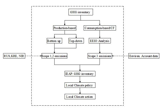
Research methods adopted in this study are illustrated by Figure 2.4: literature review,
interviews, and survey of methodologies and standards are conducted at the first stage; IEAP
standards and calculation methods from both consumption and production perspective are
then carefully chosen for the compilation of the GHG inventory; the next stage involves
statistic collection, processing and calculation, which are based on several energy and
emission databases in Sweden; finally results from both production and consumption
perspectives are analyzed and compared to guide local climate strategies.
2
http://www.h.scb.se/scb/mr/enbal/guide2/en_frame.htm
3
http://www.rus.lst.se/kartfunktion.html
4
http://www.mirdata.scb.se/MDInfo.aspx
16Figure 2.4 Methodological choice of the case study of Haninge GHG accounting
3. Results and analysis: Carbon Footprint of Haninge
3.1. Greenhouse Gas inventory of Haninge
A comprehensive GHG inventory formulated according to IEAP is presented in table 3.1. In
the table, emission sources are categorized into four sectors and three scopes.
Calculation for the energy sector is based on the Haninge energy balance table by final use
(see Appendix II) for 2008, where consumption of each fuel type and electricity is recorded
for each sector: agriculture, forestry and fishing, industry and construction, public service,
transport, household and other use. Swedish national average emission factors for each fuel
type and the Global Warming Potential (GWP) of non-CO2 Greenhouse Gases provided by
the IPCC are applied here. During the calculation, the amount of energy produced from each
type of fuel is firstly multiplied by corresponding emission factors to estimate emissions of
the three major Greenhouse Gases (CO2, CH4, and N2O). Then the amount of non-CO2 gases
emitted is converted into CO2 equivalent by multiplying by their GWP. The total GHG
emissions are a sum of all the emissions as CO2 equivalent.
17As is shown in the table, emissions from final energy use amount to 155,740 tonnes CO2 eq
for Scope 1 and 16,228 tonnes CO2 eq for Scope 2, dominating the entire GHG inventory.
Emissions from transport are the largest part of those from the energy sector. An intensive
consumption of diesel and gasoline is recorded in the transport sector, as well as a small
amount of electricity use (see Appendix II). Gasoline and diesel, mainly used as vehicle fuels,
are the largest non-biogenetic contributors to GHG emissions, resulting in over 80% of the
Scope 1 emissions. While 100% of power and heat are produced from renewable sources, the
transport sector still relies heavily on fossil fuels. There is a low proportion (approximately
5%) of ethanol blended in gasoline, but emissions from these biofuels have been deducted
from the emission of gasoline (SMED, 2009). The low consumption of biofuels in transport
indicates a potential area of improvement.
Electricity is supplied by the national grid; therefore the resulting emissions are categorized
into Scope 2. Purchased electricity, as a Scope 2 emission source, result in nearly 10% of the
total emissions from local energy use. The percentage is very small considering the fact that
purchased electricity constitutes almost half of the total energy supply of Haninge. The low
carbon intensity of Swedish electricity is due to the fact that electricity production in Sweden
is dominated (96%) by sources free of greenhouse emissions, with 85% - 90% by
hydroelectric and nuclear power generation (Sweden energy, 2010). A small amount of GHG
emission from household energy use can be seen in the table. This does not necessarily mean
that energy consumption in households is small; but is rather due to the fact is that heating
produced from biomass and electricity from renewable sources and nuclear power are
supplied to households. It is not recorded in the inventory that more than 8,600 tonnes of
biogenetic CO2 is released due to biomass combustions for household energy.
Additionally, as can be observed in the local energy balance table (Appendix II), a large
amount of biomass is used for production of district heat. Although a significant amount of
CO2 emission is caused by the combustion of biomass, it is not included in the inventor as
they are biogenice emissions from natural sources.
Emission statistics in the industrial processes, agriculture and waste sectors are derived from
the National Emission Database of RUS. A top-down approach is applied in this database,
dividingnational emission data to make it applicable at the municipality level. Emissions
attributed to the industrial processes sector are non-fuel related emissions. A small amount of
CO2 and F-gases are recorded arising from the industrial processes of Haninge. This small
climatic impact is in accordance with the lack of industries in Haninge. Beside use of energy,
the agriculture sector mainly generates CH4 and N2O emissions from stock raising. Emissions
from waste treatment as a result of local activities are allocated to the municipality from
national GHG emissions data based on population ratio. A more site-specific estimation could
be conducted if detailed data for Sofialund landfill and Stockholm sewage treatment were
obtained. For a further study data could be obtained from Henriksdal sewage treatment plant.
Emissions from waste treatment should be counted as Scope 3 emissions as both municipal
solid waste and sewage are delivered to handling facilities outside Haninge.
18The overall GHG emissions of Haninge from a production perspective, namely Scope 1
emissions, are 169,000 tonnes of CO2 equivalent for the whole municipality, and
approximately 2.3 tonnes CO2 eq per capita. The external emissions arise from production of
purchased electricity and waste treatment equal to 18% of the production-based emissions.
Additionally, one should keep in mind that a significant amount of Scope 3 emissions is not
included in the table due to lack of Input-Output statistics of consumer products for Haninge.
The critical part of Scope 3 emissions in Haninge lies in the indirect emissions caused by
imported goods in support of local consumption. Since specific data for local consumption is
not available, the analysis of consumption pattern in the following section is based on
Swedish national statistics on emissions caused by private consumption. It is believed that the
national average data is sufficient to represent the consumption pattern of Haninge residents,
and the pertinence of this analysis can be improved through qualitative adjustment based on
local social-economic statistics.
19Table 3.1(1) Greenhouse Gas Inventory of Haninge Municipality (Scope 1), 2008
Scope 1
Sector CO2(t) CH4(t) N2O(t) HFC(t CO2 eq) PFC(t CO2 SF6 (t CO2 Sum(t CO2 eq)
eq) eq)
Energy 154,029.742 21.392 4,066.7 155,739.632
Agriculture, forestry, fishing 2,861.154 0.0243 0.054 2,878.427
Industry, construction works 2,907.094 0.0288 0.065 2,927.935
Public sector 707.891 0.008 0.017 713.329
Transport 143,191.670 212.754 3.270 144,652.199
Other services 3,054.859 0.0377 0.078 3,079.731
Household 1,307.071 0.0172 0.583 1,488.013
Industry processes 111.730 4,874 10.2 72.178 5,068.108
Mineral industry 4.730
Metal industry 107
F-gases use 4,874 10.2 72.178
Agriculture 0.0 85.7 20.7 8,216.7
Ruminants 76.3
Animal manure 9.4 2.5
Other agricultural emissions 18.2You can also read