Case study: Integrated resource planning for urban water-Wagga Wagga - Institute for Sustainable Futures
←
→
Page content transcription
If your browser does not render page correctly, please read the page content below
Case study:
Integrated resource planning
            for urban water—
               Wagga Wagga

           Institute for Sustainable Futures

     Waterlines Report Series No 41, Section 7, March 2011

       NATIONAL WATER COMMISSION — WATERLINES            1
Contents
Summary ....................................................................................................................................5
1.1       Introduction ................................................................................................................6
1.2       Approach ...................................................................................................................6
1.3       Methodology ..............................................................................................................8
1.4       Discussion .............................................................................................................. 40
1.5       Conclusions ............................................................................................................ 43
1.6       References ............................................................................................................. 45
Appendix 1A: Baseline assumptions ....................................................................................... 47
Appendix 1B: Option details and assumptions ........................................................................ 58
Appendix 1C: Options results—cost breakdown ..................................................................... 73

Figures
Figure 1.1 Overview of integrated planning process for urban water                                                                         7
Figure 1.2 Schematic of groundwater movement in Wagga                                                                                     10
Figure 1.3 Study region boundary                                                                                                          11
Figure 1.4 Monthly record of bulk water delivered (kL/month)                                                                              13
Figure 1.5 Total customer metered demand, single residential households                                                                   15
Figure 1.6 Total customer metered demand, multiresidential households                                                                     15
Figure 1.7 Historical and projected population, single and multiresidential
     households                                                                                                                           17
Figure 1.8 Historical and projected number of households, single and multiresidential
     dwellings                                                                                                                            17
Figure 1.9 Baseline system yield scenarios (ML/a)                                                                                         19
Figure 1.10 Demand sectors, subsectors and end uses                                                                                       20
Figure 1.11 Time series of modelled residential end-uses—not calibrated to
     customer metered demand                                                                                                              22
Figure 1.12 Time series of modelled residential end-uses—calibrated to customer
     metered demand                                                                                                                       22
Figure 1.13 Average monthly water consumption per property—‘institutional’
     category—education                                                                                                                   23
Figure 1.14 Average monthly water consumption per property—‘other residential’
     category—hotels and motels                                                                                                           24
Figure 1.15 Average monthly water consumption per property—commercial
     properties (individually metered)                                                                                                    25
Figure 1.16 Average annual water consumption—‘industrial’ category—high water
     users                                                                                                                                25
Figure 1.17 Annual comparison of historical bulk water produced and customer
     metered demand (ML/a)                                                                                                                26
Figure 1.18 Baseline supply–demand balance for potable water in ‘licensed
     allocation’ and ‘reduced allocation’ scenarios (ML/a)                                                                                27
Figure 1.19 Baseline demand component forecast for potable water (ML/a)                                                                   28
Figure 1.20 Baseline demand composition in 2010 for average annual demand (left)
     and peak day demand (right)                                                                                                          29
Figure 1.21 Strategic supply–demand forecast for potable water subject to the
     ‘tentative’ S1 options (ML/a)                                                                                                        33
Figure 1.22 Strategic supply–demand forecast for potable water subject to the ‘more
     aggressive’ S2 options (ML/a)                                                                                                        34
Figure 1.23 Societal net unit cost curve of cumulative potable water yield for the
     ‘tentative’ S1 options                                                                                                               35
Figure 1.24 Societal net unit cost curve of cumulative potable water yield for the
     ‘more aggressive’ S2 options                                                                                                         36
Figure 1.25 Utility ‘program’ unit cost curve of cumulative potable water yield for the
     ‘tentative’ S1 options                                                                                                               37
Figure 1.26 Utility ‘program’ unit cost curve of cumulative potable water yield for the
     ‘more aggressive’ S2 options                                                                                                         38

                                                             NATIONAL WATER COMMISSION — WATERLINES                                        2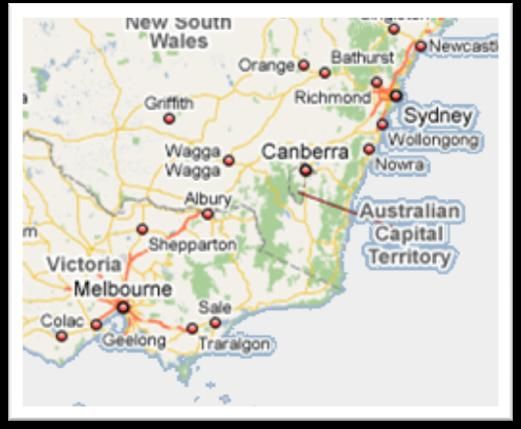
Tables
Table 1.1 Potential demand management options included in the study                    31
Table 1.2 Net present value costs and estimated GHG reductions of alternative
     strategies                                                                        39
Table 1.3 Summary cost breakdown for adjusted strategies                               40
Table 1.4 Differences in water cycle issues between coastal cities and inland cities   41

                                          NATIONAL WATER COMMISSION — WATERLINES       3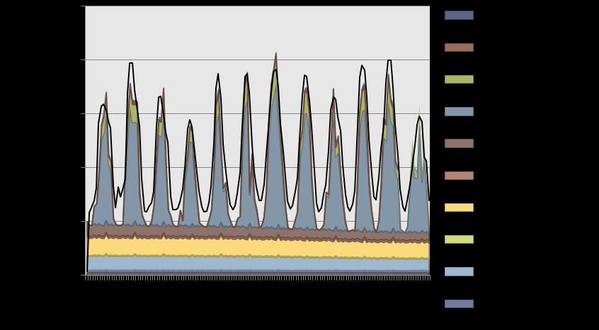
Abbreviations and acronyms
ABS            Australian Bureau of Statistics
ACT            Australian Capital Territory
CMD            customer metered demand
CO2            carbon dioxide
CSIRO          Commonwealth Scientific and Industrial Research Organisation
DSM DSS        demand-side management decision support system
GHG            greenhouse gas
HSC            HydroScience Consulting
IRP            integrated resource planning
iSDP           integrated supply–demand planning
ISF            Institute for Sustainable Futures
IWCM           integrated water cycle management
NPV            net present value
RWCC           Riverina Water County Council
SWC            Sydney Water Corporation
WSAA           Water Services Association of Australia
WWCC           Wagga Wagga City Council

Acknowledgments
The authors would like to thank Greg Finlayson and Peter Clifton at Riverina Water County
Council (RWCC) and Brad Jeffrey at Wagga Wagga City Council (WWCC) for their support
and advice on this case study. Additional thanks to Collin James at RWCC for his help with
supplying maps and identifying boundaries and Jason Ip at RWCC for his tireless work in
extracting and processing data.

                                         NATIONAL WATER COMMISSION — WATERLINES              4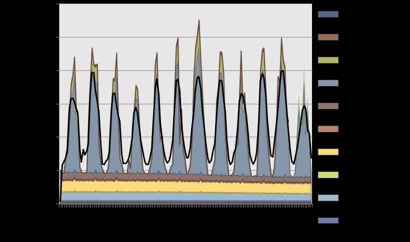
Summary
What is the purpose of this paper?
The purpose of this document is to assist Australian water resource planners to assess the
benefits and feasibility of using the integrated resource planning (IRP) process through a case
study demonstration of the regional city of Wagga Wagga in New South Wales (NSW). After
introducing the IRP process and the supporting tool, the document details each step of the
process, including the collection of data, the development of the supply–demand forecast, the
identification of options, and the analysis of the results. In so doing, the case study seeks to
reveal both the challenges and insights of the process in a real situation.

Will this paper be useful to me?
This case study complements the Guide to demand management and integrated resource
planning for urban water (Turner et al. 2010), which has been updated as part of this project.
This report will be useful for water resource decision-makers or analysts who are considering
initiating an integrated water resource planning process within their own organisations. The
case study focuses on the analytical aspects of demand forecasting and the development of
demand management options, using the integrated supply–demand planning (iSDP) model
for most of the analysis. The paper should therefore be of particular interest to readers
wanting to understand these core analytical elements of urban water supply–demand
planning and/or those considering using the iSDP model.

What are the take-home messages?
The IRP process can be used for both coastal and inland Australian cities to assess the
feasibility of water supply and demand options. It is most useful for cities that are facing a
water supply–demand gap and require a detailed analysis of options that can fill that gap.
However, as demonstrated by the case study, IRP also has value in regions with uncertain
future water availability.
A key recommendation of this case study is that future IRP studies of inland regions should
make peak day demand a focus when analysing annual average demand.
The case study also demonstrates that in the NSW context the analytical aspects of IRP and
the iSDP model can be used as part of NSW integrated water cycle management (IWCM)
planning and are complementary to an IWCM process.

                                          NATIONAL WATER COMMISSION — WATERLINES                 5
1.1 Introduction
In 2008, the Institute for Sustainable Futures at the University of Technology, Sydney, was
commissioned by the National Water Commission to undertake the Integrated Resource
Planning for Urban Water Project. This case study report is one of the components of that
project. The project has developed tools and materials that are designed to assist water
service providers with their longer term water planning. This report documents a case study
undertaken to demonstrate the analytical steps of urban water IRP, with reference to the city
of Wagga Wagga.
The objectives of the case study were to apply the analytical steps in IRP to the urban water
planning issues facing Wagga Wagga and document the implementation of the iSDP model.
This includes the analysis of input data, the development of supply–demand forecasts, the
identification of options, and the analysis of the results. The case study also aims to assess
the usefulness of the IRP framework and supporting tools for water planning in regional
centres like Wagga Wagga.
Wagga Wagga is a major inland city in southern New South Wales and is located in the
Murray–Darling Basin. Most recent applications of the IRP framework and iSDP model have
been to large coastal cities. Therefore, Wagga Wagga was selected as a case study because
it provides a good example of how the IRP framework and tools can be adapted to the unique
challenges and opportunities faced by inland regional centres.
The report begins by providing background on the IRP process and the iSDP model. It then
details each stage of the analysis and concludes with a critical evaluation of the usefulness of
the IRP framework in similar regional contexts.
1.2 Approach
1.2.1 Integrated resource planning
The project methodology is underpinned by IRP, a comprehensive decision-making process
directing the effective provision of infrastructure services to cities. The fundamental insight of
the process is that cities demand services rather than resources and that options to augment
system capacity (for example, through new sources) should therefore be compared alongside
options to control demand (for example, through efficient appliances) on an equivalent basis.
Over time, IRP has evolved to encompass other important aspects of decision-making about
public infrastructure, including public participation, explicit consideration of uncertainty and
meeting multiple objectives.
The process broadly involves establishing an agreed definition of the system and its
constraints, setting study objectives, developing a detailed baseline forecast of the demand
and capacity of the system, and then using it as a basis for assessing a broad range of both
supply-side and demand-side options. This ensures that the most cost-effective and
sustainable options are considered for implementation.
The Institute for Sustainable Future (ISF) implementation of IRP for supply–demand planning
in the urban water sector has been supported by the International Water Association (Turner
et al. 2007), the Water Services Association of Australia (Turner et al. 2008), and the National
Water Commission (Turner et al. 2010), and is summarised in Figure 1.1.
NATIONAL WATER COMMISSION — WATERLINES 6Figure 1.1 Overview of integrated planning process for urban water
1.2.2 The iSDP model
Decision-support tools fulfil an important role in IRP by facilitating the complex task of
assessing and projecting the supply–demand balance of a region, and rigorously comparing
the range of demand-side and supply-side options for meeting the study objectives.
The iSDP model was designed specifically for that task. The model was first developed by the
ISF in the late 1990s as a demand forecasting and options assessment tool to assist Sydney
Water Corporation (SWC) to undertake integrated water resource planning. The model was
subsequently improved by SWC and ISF and was later released in 2003 with the support of
the Water Services Association of Australia (WSAA). Since its release, the tool has been
improved by ISF and CSIRO with various WSAA members in major cities around Australia.
To consolidate those improvements and to engage a broader customer base beyond WSAA
members, the National Water Commission funded a significant upgrade of the model, which
in 2010 was released nationwide to utilities, councils and associated public agencies
interested in undertaking integrated water resource planning.
Key features of the model include:
integrated resource accounting of water, wastewater, energy and greenhouse gases
integrated cost accounting of costs and avoided costs borne by the customer, the
responsible utility, any relevant project partners and society as a whole
appliance stock models to project shifts in appliance efficiencies subject to new
technologies and standards
dynamic outputs capable of comparing alternative demand, baseline system yield and
option yield scenarios
transparent reporting of model assumptions and embedded supporting reference
documents.
The tool is based on a series of Excel workbooks linked to a central database and comprises
two integrated modules: a baseline forecast module and an options assessment module. The
baseline forecast module projects water demand based on a series of disaggregated
end uses, each representing individual sectors (for example, the industrial sector) or activities
(such as toilet flushing). These component forecasts are each based on a series of
assumptions relating to future changes in the mix of sectoral and housing types, and the
ownership, usage behaviour and efficiency of fixtures and appliances, among other variables.
External analysis is then applied to project the water resource capacity of the existing supply
system (or system yield), which is then input to the model. The output is a baseline forecast,
which is a ‘business as usual’ or ‘reference case’ projection of the supply–demand balance,
assuming no significant intervention by the water service provider or other authorities.
The baseline forecast then forms the basis for the options assessment module. The options
assessment module projects the augmented or avoided capacity associated with each option,
based on a series of assumptions relating to participation rates and water savings. The
economic costs borne by society as a whole, as well as the financial costs borne by the
relevant stakeholders, are then projected over the life cycle of each option. These two time-
series projections are then expressed as a unit cost ($/kL) to allow the cost-effectiveness of
options to be compared.
The final output is a series of metrics and charts that enable a balanced comparison of
options, whether they involve augmenting system capacity (for example, commissioning
additional reservoirs), avoiding the need for additional system capacity (such as by
NATIONAL WATER COMMISSION — WATERLINES 7implementing demand management programs) or a combination of the two. Critically, the
analytical outputs of the iSDP model are designed to inform the broader decision-making
process that is part of IRP for urban water, which should involve community and/or
stakeholder input.
1.3 Methodology
1.3.1 Planning the process
Establishing the
context
Wagga Wagga is Australia’s
fifth largest inland city, with a
current population of more
than 59 000. The city is
situated approximately
midway between Sydney and
Melbourne and about 2 hours
drive west from Canberra.
Wagga Wagga is on the
Murrumbidgee River and sits
in an alluvial valley that is in
the upper reaches of the
Riverina plain. The city is an
educational, retail, industrial,
retirement and military hub
within the Riverina region.
Riverina Water County Council (RWCC) is responsible for managing the urban water supplies
for four local government areas, of which the Wagga Wagga City Council (WWCC) is by far
the largest. Wastewater and stormwater are both the responsibility of the WWCC. Water is
sourced by pumping from the Murrumbidgee River (44 ML/d) and from borefields to the east,
west and north, each with a nominal rated capacity of 25 ML/d (Finlayson 2010). In 2004–05,
the Wagga Wagga urban area was using 20 ML/d in winter and up to 100 ML/d in summer.
Evaporative coolers, air-conditioners and outdoor irrigation are important contributors to peak
demand.
Driver 1: Constrained water availability and climate change
Wagga Wagga’s urban water supply is sourced from the Murrumbidgee River and from a
series of deep aquifers. The aquifers have a connection to the channel of the Murrumbidgee
River and are replenished by river flows. The relationship between the flow regime of the river
and the availability of groundwater continues to be investigated; however, the interconnection
means that constraints on available water supplies in the region apply to both surface and
groundwater sources.
Wagga Wagga is one of a string of urban and agricultural settlements, both upstream and
downstream, that are dependent on the Murrumbidgee River and its associated groundwater
aquifers. Although water availability in the region has been high in the past, in the future it is
expected to be significantly more constrained. This is due to both the reversal of historical
overallocation of water and the impact of climate change across the Murray–Darling Basin.
The Murrumbidgee River was one of the catchments covered by the CSIRO’s Murray–Darling
Basin Sustainable Yields Project, and the final report on the region was published in 2008
(CSIRO 2008). The project linked modelling of rainfall–runoff to groundwater modelling and
water use across the region under various climate and development scenarios. Connectivity
between surface and groundwaters was included. The scenarios considered included one
NATIONAL WATER COMMISSION — WATERLINES 8based on a continuation of the 1997–2006 drought, as well as scenarios incorporating best
estimates projections of water availability based on climate change modelling.
The CSIRO’s Sustainable Yields study found that the long-term average surface water
availability in the Murrumbidgee River was 4270 GL per year. About 10% of this total came
from interbasin transfers from the Snowy Mountains Hydro-electric Scheme. On average,
53% of the total surface water was diverted for use in the region, of which Wagga Wagga
urban use was only tiny fraction. The study also found that, if the drought conditions from
1997 to 2006 continued, the average surface water availability would reduce by 30%. CSIRO
applied a range of climate models to the catchment. It found that the best estimate was a 9%
decrease in runoff by 2030 (significantly less that the impact of continuing drought), but that a
level of uncertainty about future climate remained.
The guide to the Murray–Darling Basin Plan (MDBA 2010) indicates that Murrumbidgee
surface water extractions will need to decrease by between 32% and 43%. The plan holds
‘critical human need’ as the highest priority for water. However, it will be the NSW
Government’s interpretation of the Murray–Darling Basin Plan that defines the surface water
constraint for Wagga Wagga.
The local aquifer that Wagga Wagga relies on for its groundwater supply, Zone 2 of the
mid-Murrumbidgee groundwater system, is only 20 kilometres long and exhibits numerous
signs of stress (Finlayson 2010). It has highly intensive demands compared to adjacent
aquifers, and declining water levels in the bores and reduced outputs (Finlayson 2010). A
current hydrogeological modelling study, as part of RWCC’s IWCM planning (see Driver 5
below) is addressing the question of sustainable yields from the existing bores and the Zone 2
aquifer.
The CSIRO Sustainable Yields study indicated that in the mid-Murrumbidgee groundwater
system a stable groundwater level would be attained at an extraction level of about 40
GL/year (about 85% of the current usage). However, reductions might be expected to be
higher in Zone 2 (Finlayson 2010).
Any reductions in groundwater or surface water allocations are likely to leave town water
supplies secure. The NSW Department of Environment, Climate Change and Water has
stated that towns with high-security water allocations would be buffered from reductions in
inflows due to climate change (DECC 2008), and the Murray–Darling Basin Plan will make
‘critical human needs’ the top water priority (MDBA 2010). However, during the recent
drought, the NSW Government temporarily cut Wagga Wagga’s town-water allocation from
the river by approximately half and imposed restrictions on outdoor water use. Given this, the
question of water availability for urban water use in Wagga Wagga is likely to remain a
question of government allocation, and future decisions in this regard will be made in the
context of reduced water availability in the Murrumbidgee River system more generally. By
looking at the potential for demand management, this study seeks to facilitate informed
consideration of the costs and other implications of decreasing future town water allocations.
Driver 2: Urban growth
Although the boom growth period that the city experienced during the 1970s is unlikely to be
surpassed, the NSW Department of Planning is expecting moderate population increases to
2030, with an annual growth rate of 0.5–0.6% per annum over the period. Over the past two
decades, growth in housing has been higher than population growth due to declining
occupancy rates, a feature in most Australian urban areas. Between the 1991 and 2006
censuses, residential occupancy in Wagga dropped from 2.8 to 2.5. Occupancy is important,
as water uses such as garden watering are driven by housing numbers rather than
population. Growth in the industrial sector of the city is also expected, and several large
customers are currently or soon to be established.
The urban growth will lead to new demands for water services in the city. The projected
growth in services then necessitates supply–demand planning to meet that demand. Through
developing demand projections and options, this study aims to support supply–demand
planning for Wagga Wagga.
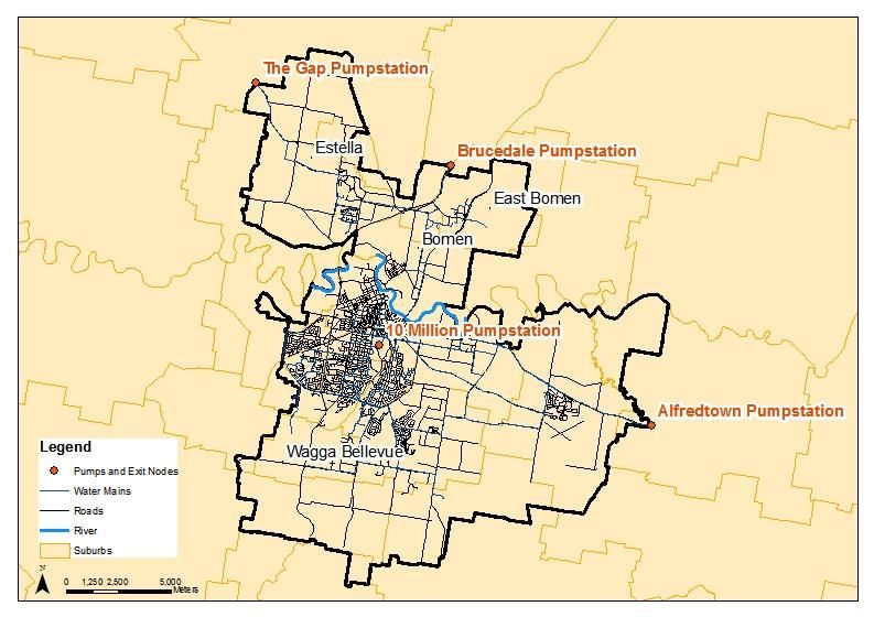
NATIONAL WATER COMMISSION — WATERLINES 9Driver 3: In-town groundwater salinity
Wagga Wagga’s naturally saline upper watertable has risen significantly since settlement
owing to historical poor land management practices, including excessive irrigation (both rural
and urban) and deforestation. The consequence has been waterlogging and salt damage to
private and public buildings, roads, and water and stormwater infrastructure, resulting in
estimated repair and maintenance costs of $183 million in present value terms over a 30-year
period (NSWDLWC 2000).
Figure 1.2 Schematic of groundwater movement in Wagga
Source: Wagga Wagga City Council (2001).
Because outdoor use is a large component of water consumption in Wagga Wagga, this study
assesses a range of outdoor demand management options. Options targeted at reducing
outdoor water consumption also present an opportunity for managing in-town salinity impacts.
Driver 4: Reducing greenhouse gas emissions
To address the issue of climate change, water utilities need to look at their energy use and
direct greenhouse gas (GHG) emissions in parallel with the impact of climate change on their
water demand and supply balance (Fane et al. 2010). As in all regions, minimising and if
possible reducing GHG emissions should therefore be considered a driver for action in water
planning for Wagga.
Driver 5: Concurrent integrated water cycle management
planning
The NSW Office of Water requires council-owned water utilities in NSW to prepare IWCM
plans. RWCC undertook an IWCM planning process concurrently with this case study. The
case study therefore aims to produce analyses that are useful for the IWCM planning.
Scoping the system
The scope of the study is limited to the assessment of the potable water demand and supply
capacity for the city of Wagga Wagga. Consequently, the study region has been limited to the
Wagga Wagga system, which is bound by the suburbs of Estella and Bomen to the north,
Alfredtown to the east, Ashmont to the west, and Bourkelands to the south. For analysis
purposes, the network boundary has been defined by the pumpstations at The Gap,
Brucedale and Alfredtown and by the 10 million gallon storage as marked in Figure 1.3.
NATIONAL WATER COMMISSION — WATERLINES 10Figure 1.3 Study region boundary
The study focuses on the long-term planning horizon. As such, it has adopted a period
beginning in the 2009–10 financial year and ending in 2049–50, with an annual time
increment. The study addresses an economic question, so a whole-of-society perspective
should be considered in relation to costs. Therefore, the study assesses the costs and
benefits borne by the utility, the customer and any third-party partners. Ideally, externalities
should also have been included. However, due to the limitations of scope, externalities were
not quantified as part of this study.
Specifying the objectives
Constraints
Consistent with the objectives of IRP for urban water supply–demand planning and the
Wagga Wagga context outlined above, the alternative strategies considered in this study were
limited by the following constraints:
In relation to surface water supply, the town water allocation cannot be exceeded. The
alternative scenarios must not withdraw water in excess of their allocations, as stipulated
by the NSW Department of Environment, Climate Change and Water.
In relation to groundwater water supply, neither the town water allocation nor the physical
limits to groundwater can be exceeded. The alternative scenarios must not withdraw
water in excess of their allocations. Current hydrogeological modelling is helping to
define the physical limit of groundwater availability.
In relation to water demand, demand for water services in the region is to be met. The
alternative strategies must provide sufficient water to meet the forecast water service
requirements of the future population, either by increasing supply or by managing
demand.
NATIONAL WATER COMMISSION — WATERLINES 11Principal objectives
Within the constraints outlined above, the principal objectives of the study were to:
1. identify options that may be economically cost-effective from the perspective of the
society as a whole
2. assess the potential to reduce demand cost-effectively in order to meet the water supply
constraint in a potential future scenario in which allocations need to be reduced
3. identify options that may be financially cost-effective from the perspective of the water
supply utility (RWCC).
The cost-effectiveness of options was evaluated in this study based on the levelised unit cost
of water. This is the present value of the cost of the option (whether to society as a whole or
to the water utility) divided by the present value of the annual volume of water saved or
supplied by the option (Dziegielewski et al. 1992:109, Fane et al. 2003, Herrington 2006).
Based on the levelised unit cost, an option’s cost-effectiveness can be assessed relative to
the marginal cost of water supply in the study region.
Secondary objectives
The secondary objectives for the study were to:
1. minimise potential amenity losses due to options that affect lawns and gardens
2. identify options that reduce outdoor demand and would also have a positive impact on
urban salinity
3. identify options that that could reduce GHG emissions.
Amenity loss and reduced outdoor demand in relation to in-town salinity were assessed
qualitatively, while GHG emissions where estimated quantitatively in terms of total emissions
to 2050 in carbon dioxide equivalents (CO2-e).
1.3.2 Analysing the situation
Collecting the information
After the analytical basis for the study was established, the next stage involved gathering,
processing and analysing sufficient data to inform the analysis.
The key data inputs to the analysis were:
bulk meter data—high-resolution, aggregated consumption data recorded at the water
treatment plant
customer meter data—lower resolution consumption data recorded at individual
customer connections
demographic data—historical and projected population, household occupancy and other
attributes of the region
end-use data—customer surveys and measurement studies to characterise water-use
behaviour
climatic data—meteorological records characterising rainfall, evaporation rates,
temperature etc.
The analyses performed and their results are detailed below.
Bulk meter data
Bulk meter data represents the total water produced by the system. This data can be
compared with the customer metered demand (CMD) data to determine system losses. Bulk
meter data is typically available at more highly resolved time steps than CMD data and
NATIONAL WATER COMMISSION — WATERLINES 12therefore is a more accurate basis for analysing time-variable influences on demand, such as
seasonality and the effect of major events such as drought.
Using its existing bulk meter data collection system and a subsequent round of data
cleansing, RWCC was able to provide monthly time series of bulk water delivered to the
Wagga Wagga system, as shown in Figure 1.4.
Figure 1.4 Monthly record of bulk water delivered (kL/month)
Note: The system retains several anomalies that suggest spurious meter reads.
ISF recommends that utilities starting a water planning process invest time in improving bulk
meter data accuracy as an initial step.
Customer meter data
Customer meter data is used for several purposes; first, it is compared with bulk water
demand to help determine system losses between the bulk meter and customer connections;
second, it is used as the calibration point for the modelling of residential end-uses; third, it is
used as direct input in the model for the non-residential sector.
Customer meter data has historically been collected for billing purposes and, although the
quality of the data varies, some form of preprocessing and data validation is usually required.
The following preliminary tests were applied to the customer meter data to determine where
corrections and/or data cleaning were required:
1. reversed read dates
2. read dates outside expected range
3. read period outside expected range
4. read period discontinuous
5. negative consumption
6. consumption outside expected range.
The tests revealed a significant proportion of records with reversed dates and negative
consumption. Those records were subsequently identified as metering corrections, which
NATIONAL WATER COMMISSION — WATERLINES 13were removed by switching the dates and summing the records by read period to yield a
corrected meter read.
Where tests identified clearly spurious data, which for the most part involved those records
identified in the date range test, the offending records were identified and excluded from the
dataset.
The quarterly customer meter data was then ‘binned’ or apportioned to individual months to
provide a better indication of the temporal distribution of demand. This is possible because
customer meters are read over different periods that are spread roughly evenly across the
year. The process is associated with some artificial smoothing of the time-series, but for large
numbers of customers that effect is less pronounced.
The process for binning customer meter data was as follows:
1. The mean daily consumption rate for each quarter was calculated for each individual
customer.
2. The monthly consumption for each customer was then calculated by adding the daily
consumption rates that fall within that month. If the meter was not read in that month, the
monthly consumption would simply be the daily consumption rate multiplied by the
number of days in that month, whereas if the meter was read within that month the
monthly consumption would represent a weighted average consumption rate prorated
with the number of days of each intersecting meter read period that fell within the month).
3. The significant errors of the binning process were then reduced by calculating the mean
binned monthly consumption by customer type to provide a smoothed estimate of
monthly time-series demand.
For more details on the process of binning, refer to Appendix B of the Guide to demand
management and integrated resource planning (Turner et al. 2010).
The binned monthly consumption for both single and multiresidential households is shown in
Figure 1.5 and Figure 1.6. The relatively high seasonality is a consequence of the high
temperatures and evaporation rates in the summer months. Note that the available data in the
2003–04 period appears to have been incomplete and should be considered as a data
anomaly.
NATIONAL WATER COMMISSION — WATERLINES 14Figure 1.5 Total customer metered demand, single residential households
Figure 1.6 Total customer metered demand, multiresidential households
NATIONAL WATER COMMISSION — WATERLINES 15Demographic data
The demographic characteristics of the service area are the major influence on future demand
and therefore the foundation of the analysis.
The key demographic inputs to the iSDP model are:
historical census data characterising the population, dwellings, dwelling structure
(detached, semidetached, flats or apartments) and dwelling occupancy (occupants per
dwelling) etc.
projected population, dwellings and occupancy levels.
This data was entered into the region sheet within the model and formed the basis of the
water use projections.
The historical census data is typically provided by the Australian Bureau of Statistics in a
variety of resolutions, ranging from highly aggregated regional data tables for periods prior to
the 1996 Census, to the geographically referenced datasets of subsequent censuses that
provide data by census collector district (approximately 500 households).
The projected populations, dwellings and occupancy ratios are typically provided by the
relevant state authority (in this case, the NSW Department of Planning) and are typically
1
available by statistical local area (approximately 15 000 households) (NSWDP 2005).
As the regions of the historical and projected datasets rarely align with the service area in
question, spatial analysis is necessary for both datasets.
To begin, a spatial database query was applied to select those statistical collector districts in
the most recent ABS census basics dataset (ABS 2006) with centroids lying within the service
area boundary. After the districts were selected, the population and household counts by
dwelling structure were then summed for single residential households (those households
living in detached dwellings) and multiresidential households (those living in other dwelling
structures, including semidetached dwellings, flats and apartments).
This process was then repeated for the demographic projections (obtained from the
Department of Planning) to derive an annual time-series forecast of population. As no
projections of dwelling numbers were available, these figures were derived by assuming that
household occupancy within single and multiresidential dwellings will remain unchanged in
the future.
The historical time series to 1960 represents the aggregated population of Wagga with an
unspecified boundary, so this data was drawn directly from the dataset. In the absence of
readily available dwelling counts, the figures were derived by applying nationwide historical
occupancy levels.
The annual time series were then entered into the region sheet within the iSDP model, which
applies the recent census year data as the base year and the historical and projected time
series as forecast and hindcast factors to provide a consistent time series. Those projections
resulted in a characterisation of key demographic attributes for the study region for the period
2
from 1960 to 2050. The projection of population in single and multiresidential dwellings is
shown in Figure 1.7, while the numbers of dwellings within each housing type are shown in
Figure 1.8.
1
Some more highly resolved projections may be acquired from various state government agencies.
2
Note: The hindcast to 1960 is necessary to establish the mix of ages of dwellings and appliances for
stock modelling purposes (detailed in Section 7.3.2).
NATIONAL WATER COMMISSION — WATERLINES 16Figure 1.7 Historical and projected population, single and multiresidential households
Figure 1.8 Historical and projected number of households, single and multiresidential
dwellings
NATIONAL WATER COMMISSION — WATERLINES 17End-use data
Customer surveys and measurement studies characterising water-use behaviour are
becoming increasingly available to facilitate a deeper understanding of the influences of water
demand.
Given the absence of any studies of this kind within the study area, the model relies on the
best available proxy, pending more region-specific data. Key sources included:
a state-wide survey series of household ownership for various water-consuming
appliances, conducted since 1990 (ABS 2007, 2008)
a state-side sales inventory for a number of appliances, conducted by Energy Efficient
Strategies over the period from 1993 to 2005 (EES 2006)
an extensive survey of household water use behaviour and an end-use measurement
study, both conducted by Yarra Valley Water (Roberts 2004, 2005)
several complementary surveys in Sydney and Perth (Loh and Coghlan 2003).
This data has been built into the iSDP model and is available as a default. Where no suitable
proxy was available, ISF contacted local businesses. A detailed account of the model
assumptions has been provided as Appendix 7B.
ISF recommends that, in regions with water availability constraints, studies be undertaken to
confirm specific local end-use assumptions and regionally specific variables. For instance, the
assumed shower flow rates are both highly sensitive and regionally specific (typically, they
are dependent on local water pressure) and thus a priority data gap. Evaporative cooler use
and settings are also highly specific to local conditions.
Climate data
Climate data is used both within the baseline forecasting module and within the options
assessment module.
Thirty-year daily temperature, rainfall and pan evaporation records were obtained from the
Australian Bureau of Meteorology for the weather station at Wagga Wagga AMO. That data
was inserted into the outdoor end-use sheet for use in calculating the outdoor demand
component of the baseline. The same data was also used in the various option sheets that
relate to outdoor water use to assess potential yield from demand management options
designed to reduce outdoor water use.
Modelling the system
Modelling system yield
Two system yield scenarios were assessed in the study: the ‘licensed allocation’ scenario,
which assumes that the full historical town water allocation will be maintained, and the
‘reduced allocation’ scenario, which assumes reduced allocations for both surface and
groundwater.
The ‘licensed allocation’ scenario is 7000 megalitres per annum (ML/a) available from surface
water sources and 14 000 ML/a from groundwater sources, providing a total allocation of
21 000 ML/a.
3
The ‘reduced allocation’ scenario assumes a reduction to 50% and 70% of the surface water
and groundwater sources, respectively, providing a total allocation of 13 300 ML/a.
3
Note that the 70% is an assumption made for the purposes of this case study. As part of the current
IWCM planning process by RWCC, there is a hydrogeological modelling study addressing the question
of sustainable yields from the existing borefield.
NATIONAL WATER COMMISSION — WATERLINES 18Figure 1.9 Baseline system yield scenarios (ML/a)
Modelling system demand
The demand forecast broadly comprises residential demand, non-residential demand and
non-revenue water, as depicted in Figure 1.10. Within residential demand, end uses are split
between indoor and outdoor, with outdoor demands being far more dependent on climate
variables. The calculation of residential demands is based on demographics, end use and
stock modelling undertaken within the model.
The non-residential demands are categorised as ‘industrial’, ‘commercial’, ‘institutional’,
‘recreational’ or ‘other residential’. Further subsectors break down demands according to
end-use type (for example, ‘education’ or ‘hotels’) and level of water use (such as average
user or intensive user). The model user is required to process the non-residential customer
demand data, such that it is broken down into these categories, so that it can be entered into
the model.
The non-revenue water category comprises ‘real losses’, ‘apparent losses’ and ‘unbilled
authorised consumption’. The model determines the total volumes of non-revenue water from
the difference between the bulk water and customer metered demand. The model user is
required to input factors into the non-revenue water end-use sheet so that the model can then
determine the likely breakdown of real and apparent losses and unbilled authorised
consumption.
NATIONAL WATER COMMISSION — WATERLINES 19Figure 1.10 Demand sectors, subsectors and end uses
NATIONAL WATER COMMISSION — WATERLINES 20Residential demand
The residential component of the model comprises a series of individual end uses, each
representing a water-consuming activity around the home.
The analysis of each end use is based on a series of assumptions relating to the usage
behaviour, the appliance stock mix, and the associated technology (or efficiency). These are
combined to determine the demand associated with that end use, as described by the
function:
Demand = Usage × Stock × Technology
The major indoor end-uses, including showers, washing machines, dishwashers and toilets,
use an appliance cohort stock modelling approach. This involves simulating the appliance
stock over time, based on a series of individual cohorts purchased in each year. The result is
a series of region-specific stock models for each end use. (For further details on stock
modelling and its use in demand forecasting and options development, refer to Turner et al.
2010.) Evaporative coolers are shown as ‘outdoor demand’ in Figure 1.10, in recognition of
the location of this water use and its seasonal nature. They are classified in this manner
despite the benefits of cooling occurring indoors. Evaporative coolers were modelled based
on the available literature as well as interviews with a number of suppliers and technicians
servicing coolers in the region.
The other outdoor end-uses, including lawns, gardens and pools, use a mass balance
modelling approach based on area and behaviour assumptions, coupled with historical
climate data. This involves simulating both the losses from the lawn–garden–pool system
(evaporation, transpiration etc.) and the gains to that system (rainfall, potable demand etc.).
Any difference between the losses and gains to that system results in a change in the
system’s storage (for example, the soil mass or the water reservoir in a pool).
See Appendix 1A: Baseline assumptions for details of the end-use assumptions used in the
study.
Residential calibration
After the dynamical or ‘bottom up’ model of residential demand has been created, the outputs
of the model are then calibrated to the customer meter data (analysed above, under
‘Customer meter data’), to form the ‘top down’ or empirical basis for demand. As the estimate
of baseline lawn and garden water demand is the most sensitive and variable parameter in
the residential demand forecast, this baseline component is fitted to customer metered
demand using an ‘overwatering’ factor. A graphical depiction of this process is provided
below.
Figure 1.11 shows the time series of the modelled indoor residential end-uses (flat sections of
the graph unaffected by seasonal demand) and the modelled outdoor demands (peaked
components of the graph). The black line shows the total residential customer metered
demand for that period. The calculation of lawn and garden demand includes a factor that can
be used to account for overwatering. In this graph, no overwatering factor is added and it
therefore shows ‘ideal’ watering behaviour.
While the soil moisture balance was undertaken on a daily basis, the estimated consumption
was binned into months to allow calibration with the monthly binned customer meter data.
Figure 1.11 and Figure 1.12 show daily rates to avoid artefacts caused by figures for different
days per month.
NATIONAL WATER COMMISSION — WATERLINES 21Figure 1.11 Time series of modelled residential end-uses—not calibrated to customer
metered demand
In Figure 1.12, the overwatering factor has been added so that the sum of the modelled
end-uses (indoor and outdoor) matches the total customer metered demand. This is the
calibrated version. It indicates some overwatering in current watering practice in Wagga
Wagga, but also that the larger gains are likely to be made in changing garden type than in
perfecting watering behaviours. Note that the customer metered demand is recorded at
quarterly intervals, and the process of binning this data into monthly time series has the effect
of levelling the troughs and peaks. Therefore, the difference between metered and modelled
demand on a monthly basis is exaggerated.
Figure 1.12 Time series of modelled residential end-uses—calibrated to customer metered
demand
NATIONAL WATER COMMISSION — WATERLINES 22Non-residential demand
The non-residential demand components of the model are much simpler. Non-residential
customer metered demand must be preprocessed so that properties are categorised
according to end-use type, and the highest water users in each category are extracted. Those
categories can then be entered into the relevant non-residential end-use sheets in the model.
The breakdown of non-residential end use categories is outlined in Figure 1.10.
Extracting the highest water users in each category has several purposes: first, to ensure that
average water consumptions can be determined for each category without being skewed by
very high water users; second, to identify the high water users to determine where large water
savings might be made through demand management interventions; third, to ensure that
water demand from those users can be projected individually, based on local knowledge. For
example, a factory may be making a major extension of its processes or a specific industry
might be closing down, and those events may significantly affect water use in the respective
categories. Also, some businesses and buildings are likely to expand with population growth
and others are not, so, depending on the characteristics of each customer, the predicted
demand for each individual intensive customer is either pegged to population growth or fixed
to remain constant into the future.
Once entered into the model, demand for each subsector is forecast by the model by
projecting the number of subsector customers in proportion to population growth and then
applying the mean annual consumption per customer over an appropriate calibration period.
Processing the non-residential data and determining the average water use per property for
the various categories (such as schools, hospitals etc.) also provides an insight into the
relative water use of each sector and any trends that may have been occurring in average
water usage per property in each sector. These observations become useful when selecting
demand management options that target specific sectors. A selection of graphs that were
prepared during the data preprocessing is shown below. Figure 1.13 shows the peaky nature
of water demand for educational facilities in Wagga, with average demand oscillating between
200 kL/property/month and 1000 kL/property/month. The peaks are likely to be due to outdoor
irrigation, which is primarily required during the hotter months. Demand management
programs that target irrigation efficiency are likely to help reduce the peaks.
Figure 1.13 Average monthly water consumption per property—‘institutional’ category—
education
NATIONAL WATER COMMISSION — WATERLINES 23Figure 1.14 Average monthly water consumption per property—‘other residential’ category—
hotels and motels
Figure 1.14 shows the average water consumption for hotels and motels between 2002 and
2007. This graph appears to show that the seasonal peaks in this sector are diminishing, but
that may be an artefact of the data. The graph shows that there are approximately 50
properties in this category that could be targeted for improved water management.
The average monthly water consumption for commercial properties is shown in Figure 1.15.
These properties also appear to show a seasonal peak in water use, with the average
doubling from 50 kL/property/month up to approximately 100 kL/property/month. This would
be due to a combination of evaporative air cooling and outdoor irrigation.
NATIONAL WATER COMMISSION — WATERLINES 24Figure 1.15 Average monthly water consumption per property—commercial properties
(individually metered)
Apart from the analysis of individual sectors, high water users were also extracted from the
data. Figure 1.16 shows the water consumption of the largest industrial users in Wagga
Wagga. The volume of water used at a number of these properties is significant, and any
opportunities to improve water-use efficiency could be correspondingly significant. Another
opportunity would be to determine the reason for the increase in consumption for property
no. 3, as it may represent a change in activities within the property, which could be readjusted
to reduce water use to its former levels.
Figure 1.16 Average annual water consumption—‘industrial’ category—high water users
NATIONAL WATER COMMISSION — WATERLINES 25ISF recommends that the non-residential demand projections be adjusted as new information
becomes available (for example, with the loss or addition of a major manufacturing industry).
Non-revenue water
The non-revenue water forecast in the model is based on the difference between the time
series of metered bulk water production and customer metered consumption. The annual time
series is shown in Figure 1.17.
Figure 1.17 Annual comparison of historical bulk water produced and customer metered
demand (ML/a)
In the analysis, non-revenue water is defined as the difference between the bulk water
produced and the customer metered demand. Based on the assumption that the share of
non-revenue water will remain the same, the difference between these two time series (as a
share of customer metered demand) was therefore applied as a factor to the total modelled
demand from all other demand components to yield the forecast non-revenue water demand.
Noting the relatively low customer meter data in 2003–04, during this period RWCC
implemented a program of metering improvement, which included installing meters on
multiresidential dwellings. RWCC also experienced data export issues for that year due to a
changeover in customer billing databases. Due to the apparent anomaly, the data presented
in Figure 1.17 will be reviewed as part of RWCC’s IWCM process.
Specifying the baselines
This stage involves the combination of the various baseline demand components and
baseline system yield scenarios to form a baseline supply–demand forecast, shown in Figure
1.18. Note that no supply–demand gap is forecast to occur in the ‘licensed allocation’ yield
scenario; however, in the assumed ‘reduced allocation’ scenario, a supply–demand gap is
forecast to occur beyond 2017.
Figure 1.19 shows the components of the baseline demand forecast out to 2050. Figure 1.20
depicts the current (2010) baseline composition of potable demand for both the average
annual and the peak day demand. The most obvious features of these figures are the
dominance of residential irrigation as a share of total and peak day urban water demand, and
the fact that future demand growth is being driven by growth in residential irrigation.
NATIONAL WATER COMMISSION — WATERLINES 26Figure 1.18 Baseline supply–demand balance for potable water in ‘licensed allocation’ and ‘reduced allocation’ scenarios (ML/a)
NATIONAL WATER COMMISSION — WATERLINES 27Figure 1.19 Baseline demand component forecast for potable water (ML/a)
NATIONAL WATER COMMISSION — WATERLINES 28Figure 1.20 Baseline demand composition in 2010 for average annual demand (left) and peak day demand (right)
NATIONAL WATER COMMISSION — WATERLINES 291.3.3 Developing the response
Identifying the options
Once the baseline supply–demand forecast has been established, the next stage of the
analysis is to identify a suite of potential options and to assess them in relation to the
objectives as outlined in Section 1.4.1. While the IRP assessment framework and iSDP model
facilitate a comparison of supply-side and demand-side options, in this study only
demand-side options were identified as having potential. This was because no immediate
supply-side options were evident and there was no supply–demand gap projected under the
‘licensed allocation’ water availability scenario.
A broad suite of demand management and water conservation options was identified across
the various sectors. Options were grouped into two alternative strategies: S1 (‘tentative’) and
S2 (‘more aggressive’). This was done in order to get a sense of the range of potential
responses that might be implemented and to reflect the level of action that might be taken in
the current situation with the licensed allocation and in a reduced allocation scenario. Some
options were included in both strategies, but with differing assumptions concerning take-up
rates and the corresponding effort required to drive take-up. The options are described in
Table 1.1, with ticks used to indicate relative uptake. A double tick indicates that a more
comprehensive version of the option has been included. The full assumptions used in
modelling them can be found in Appendix 1B: Option details and assumptions.
NATIONAL WATER COMMISSION — WATERLINES 30Table 1.1 Potential demand management options included in the study
Option Description Inclusion in strategy
S1 S2
1 Showerhead Householders bring their old showerhead to a shopfront –
swap location and swap it for a new one, free of charge
2 Residential Plumber visit—replace showerheads, install tap flow –
retrofit regulators (kitchen and bathroom), toilet displacement
device or cistern weight in single flush toilet; check for
leaks and provide advice
3 Toilets Complete toilet replacement (this option is currently
replacement being trialled in Wagga)
4 Clothes Rebate for replacing top loaders with 5-star front
washer loaders.
rebate
5 Evaporative Maintenance visit and education campaign (turn them
coolers down, turn them off when not at home)
6 Residential Rebate for relandscaping of nature strip (this option is
nature strips currently being developed in Wagga)
7 Outdoor DCP banning irrigated lawns –
watering
(DCP)
8 Rainwater 5 kL tank retrofit for existing residential toilets, washing –
tank rebate machines and outdoor uses (currently available)
9 Permanent No fixed sprinklers allowed between 10 a.m. and 5 p.m.
water All requested to reduce water consumption by 20% (this
conservation option has been adopted in Wagga)
measures
10 Non-revenue Leak detection and repair, pressure management
program (from Sydney Water program)
11 Water Water audit, install efficient fixtures and sensors and
audit—hotels carry out air-conditioning maintenance. Proportion of
total 49 hotels/motels
12 Water Monitoring, alarm systems for leaks, plus education. All
audit— 36 schools
schools
13 Water Water audits and modifications for five high water users
audit—
industrial
customers
14 Commercial Rebate for relandscaping of commercial properties
nature strips
Assessing the alternatives
The results of the options assessment are shown in the graphs below. Figure 1.21 and Figure
1.22 depict the supply–demand forecasts for potable water, including the reduced demand
associated with the S1 (tentative) and S2 (more aggressive) strategies, respectively.
Figure 1.23 and Figure 1.24 depict ‘cost curves’ of cumulative potable water yield due to a
range of demand management options in 2020 against the cost of water for the S1 ‘tentative’
and S2 ‘more aggressive’ strategies, respectively. Both the water utility’s and the customer’s
costs and avoided costs are included in order to approximate a whole-of-society cost. The
costs include equipment, implementation, marketing, management and post-program
evaluation. The avoided costs include operating costs (the water utility’s electricity and
chemical costs in water supply and wastewater treatment, and the customer’s costs for
heating water). Externality costs have not been included in this analysis. It was also not
possible to included potentially avoided capital costs.
NATIONAL WATER COMMISSION — WATERLINES 31You can also read