From weak to intense downslope winds: origin, interaction with boundary-layer turbulence and impact on CO2 variability - atmos-chem-phys.net
←
→
Page content transcription
If your browser does not render page correctly, please read the page content below
Atmos. Chem. Phys., 19, 4615–4635, 2019
https://doi.org/10.5194/acp-19-4615-2019
© Author(s) 2019. This work is distributed under
the Creative Commons Attribution 4.0 License.

From weak to intense downslope winds: origin, interaction with
boundary-layer turbulence and impact on CO2 variability
Jon Ander Arrillaga1,* , Carlos Yagüe1 , Carlos Román-Cascón1,2 , Mariano Sastre1 , Maria Antonia Jiménez3 ,
Gregorio Maqueda1 , and Jordi Vilà-Guerau de Arellano4
1 Departamento   de Física de la Tierra y Astrofísica, Universidad Complutense de Madrid, Madrid, Spain
2 Laboratoire d’Aérologie, CNRS, Université de Toulouse, CNRS, UPS, Toulouse, France
3 Departament de Física, Universitat de les Illes Balears, Palma, Spain
4 Meteorology and Air Quality Group, Wageningen University, Wageningen, the Netherlands
* Invited contribution by Jon Ander Arrillaga, recipient of the EGU Nonlinear Processes in Geosciences Outstanding Student

Poster Award 2015.

Correspondence: Jon Ander Arrillaga (jonanarr@ucm.es)

Received: 6 September 2018 – Discussion started: 17 October 2018
Revised: 21 March 2019 – Accepted: 22 March 2019 – Published: 8 April 2019

Abstract. The interconnection of local downslope flows of        weakly stable boundary layer. On the contrary, when the dy-
different intensities with the turbulent characteristics and     namical input is absent, buoyancy acceleration drives the for-
thermal structure of the atmospheric boundary layer (ABL)        mation of a katabatic flow, which is weak (U < 1.5 m s−1 )
is investigated through observations. Measurements are car-      and generally manifested in the form of a shallow jet below
ried out in a relatively flat area 2 km away from the steep      3 m. The relative flatness of the area favours the formation
slopes of the Sierra de Guadarrama (central Iberian Penin-       of very stable boundary layers marked by very weak tur-
sula). A total of 40 thermally driven downslope events are se-   bulence (u∗ < 0.1 m s−1 ). In between, moderate downslope
lected from an observational database spanning the summer        flows show intermediate characteristics, depending on the
2017 period by using an objective and systematic algorithm       strength of the dynamical input and the occasional interac-
that accounts for a weak synoptic forcing and local downs-       tion with down-basin winds. On the other hand, by inspect-
lope wind direction. We subsequently classify the downslope      ing individual weak and intense events, we further explore
events into weak, moderate and intense categories, accord-       the impact of downslope flows on CO2 variability. By relat-
ing to their maximum 6 m wind speed. This classification         ing the dynamics of the distinct turbulent regimes to the CO2
enables us to contrast their main differences regarding the      budget, we are able to estimate the contribution of the differ-
driving mechanisms, associated ABL turbulence and thermal        ent terms. For the intense event, indeed, we infer a horizontal
structure, and the major dynamical characteristics. We find      transport of 67 ppm in 3 h driven by the strong downslope
that the strongest downslope flows (U > 3.5 m s−1 ) develop      advection.
when soil moisture is low (< 0.07 m3 m−3 ) and the synoptic
wind not so weak (3.5 m s−1 < V850 < 6 m s−1 ) and roughly
parallel to the direction of the downslope flow. The latter
adds an important dynamical input, which induces an early        1   Introduction
flow advection from the nearby steep slope, when the local
thermal profile is not stable yet. Consequently, turbulence      Thermally driven slope winds develop in mountainous ar-
driven by the bulk shear increases up to friction velocity       eas, when the large-scale flow is weak and skies are clear,
(u∗ ) ' 1 m s−1 , preventing the development of the surface-     allowing greater incoming solar radiation during daytime
based thermal inversion and giving rise to the so-called         and larger outgoing longwave radiation during the night
                                                                 (Zardi and Whiteman, 2013). In this situation, wind direction

Published by Copernicus Publications on behalf of the European Geosciences Union.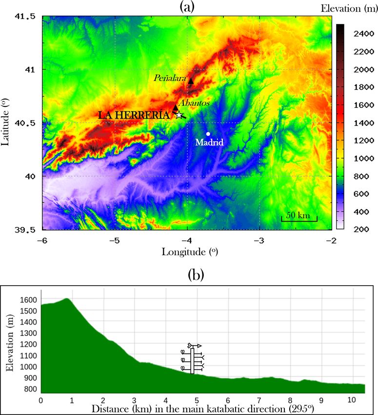
4616                                 J. A. Arrillaga et al.: From weak to intense downslope winds: origin and interactions

is reversed twice per day: thermally driven winds flow ups-        which they attributed to the sensitivity of the soil-moisture
lope during the day and downslope during the night (Atkin-         parameterisation in the numerical simulations. As a matter
son, 1981; Whiteman, 2000; Poulos and Zhong, 2008). The            of fact, Sastre et al. (2015) showed with a numerical experi-
thermal disturbances that produce them have different scales       ment at contrasting sites that soil-moisture differences do not
and origins: from local hills and shallow slopes (Mahrt and        affect the afternoon and evening transition values with the
Larsen, 1990) to large basins and valleys which extend hor-        same intensity but depend on the site. With respect to the
izontally up to hundreds of kilometres (Barry, 2008). The          background flow, by using a one-dimensional model, Fitzjar-
different scales, however, are not independent; for instance,      rald (1984) observed that the onset time of katabatic winds
local downslope flows converge at the bottom of the val-           is affected by the retarding effect of the opposing synoptic
leys generating larger-scale flows, which in turn influence the    flow and reduced cooling rates. Jiménez et al. (2019) found
mountain–plain circulations.                                       that moderate background winds in the direction of the ther-
   Mountainous sites have struck the attention of many stud-       mally driven flow enhance the latter by adding a dynamical
ies for plenty of reasons: in particular due to the influence      component.
on fog formation (Hang et al., 2016) and diffusion of pol-            On the other hand, knowing whether a certain night the
lutants (Li et al., 2018), and also due to the important role      downslope flows will be weak or intense enables us to pre-
that slope flows play in the thermal and dynamical structure       dict how turbulence in the SBL will behave. It is well known
of the atmospheric boundary layer (ABL) and its morning            that under weak large-scale wind, turbulence is weak and
and evening transitions (Whiteman, 1982; Sun et al., 2006;         patchy (Van de Wiel et al., 2003, 2012a; Mahrt, 2014), giv-
Lothon et al., 2014; Lehner et al., 2015; Román-Cascón et al.,     ing rise to the so-called very stable boundary layer (VSBL).
2015; Jensen et al., 2017).                                        On the contrary, when the large-scale wind is strong, shear
   In this work, we focus on the locally generated thermally       production increases substantially and turbulence is contin-
driven downslope winds (i.e. not driven by the basin or val-       uous, producing near-neutral conditions in the SBL (Mahrt,
ley) during nighttime and the external factors and physical        1998; Sun et al., 2012; Van de Wiel et al., 2012b) and the
processes driving their formation and subsequent evolution.        so-called weakly stable boundary layer (WSBL). Being able
The latter is closely linked to the turbulent characteristics of   to foresee the occurrence of these two regimes has been in
the stable boundary layer (SBL) and the variability of CO2 .       the eye of many studies, and some attempts have been made
Several external factors have been documented to affect these      to characterise the transition between the regimes using di-
downslope winds: the steepness of the slope and the distance       verse criteria such as the geostrophic wind (Van der Linden
to the mountain range (Horst and Doran, 1986), the canopy          et al., 2017), local (Mahrt, 1998) and non-local scaling pa-
layer (Sun et al., 2007), spatial variations in soil moisture      rameters (Van Hooijdonk et al., 2015), and the wind speed
(Banta and Gannon, 1995; Jensen et al., 2017) and the di-          (Sun et al., 2012). More or less directly continuous turbu-
rection and intensity of the synoptic wind (Fitzjarrald, 1984;     lence in the SBL has been linked with a stronger background
Doran, 1991). However, most of the investigations analysing        wind (e.g. > 5–7 m s−1 in Van de Wiel et al., 2012b) and low-
the influence of those external factors are carried out us-        level jets (Sun et al., 2012), or even with occasional irrup-
ing numerical simulations, and there is a lack of observa-         tion of sea-breeze fronts (Arrillaga et al., 2018). Our second
tional studies to validate them. Oldroyd et al. (2016) stressed    aim is therefore to explore the direct implication of thermally
the importance of adequately describing the conditions un-         driven downslope winds generated by the presence of steep
der which pure thermally driven or katabatic flows form vs.        topography, in the occurrence of the two SBL regimes.
downslope winds which have a partial dynamical contribu-              A relevant aspect of our site is its location in a relatively
tion (further described in Chrust et al., 2013). From our ob-      small flat area close to the mountain range. We therefore en-
servational analysis of several events, we particularly focus      counter a scenario different from other sites located at slopes
on how soil moisture and the large-scale wind affect the on-       where the SBL barely becomes very stable, since the shear
set time, nature and different intensities of thermally driven     production linked with the downslope wind is large and con-
downslope winds, from an observational analysis of several         tinuous, and buoyant turbulence production may occur even
events.                                                            when the stable stratification is present (Oldroyd et al., 2016).
   Soil moisture acts by enhancing or reducing the thermal         At our site, however, VSBLs associated with relatively strong
component, whereas the large-scale flow introduces a dy-           surface-based thermal inversions take place occasionally.
namical input which can considerably intensify downslope              Connected also to the dynamics of the SBL, another rele-
winds and modify their onset time. Banta and Gannon (1995)         vant issue on this topic is the impact of downslope winds of
carried out numerical simulations using a two-dimensional          different nature on the concentration of scalars of high rele-
model and found that katabatic flows are weaker over a moist       vance such as the CO2 . Previous studies have documented its
slope than over a dry one. They quantified a greater down-         influence in coastal areas (Cristofanelli et al., 2011; Legrand
ward longwave radiation and soil conductivity under moister        et al., 2016) and mountainous regions (Sun et al., 2007;
conditions, which gives rise to a reduced surface cooling.         Román-Cascón et al., 2019). Sun et al. (2007) found that
However, Jensen et al. (2017) found an opposite correlation,       downslope flows transported CO2 -rich air from the Rocky

Atmos. Chem. Phys., 19, 4615–4635, 2019                                             www.atmos-chem-phys.net/19/4615/2019/
J. A. Arrillaga et al.: From weak to intense downslope winds: origin and interactions                                             4617

Mountains, and Román-Cascón et al. (2019) observed that
horizontal CO2 advection can be relatively important over
heterogeneous surfaces affected by different emission areas.
Not only advection but also local turbulence fluxes can be
influenced: Sun et al. (2006) observed an anomalous posi-
tive CO2 flux just after sunset, suggesting that it was due to
the sudden transition from upslope to downslope flow. Be-
ing able to better quantify the influence of mesoscale flows
on the CO2 budget can help to reduce the large discrepancy
from modelling studies in reproducing the land–atmosphere
exchange for this gas (Rotach et al., 2014).
   The aim of this work is to increase in the knowledge of
    1. the external factors and physical processes that mod-
       ulate the onset time and nature of thermally driven
       downslope flows,
    2. the interaction of these downslope winds with local tur-
       bulence and the implication in the characteristics of the
       SBL and
    3. the role of advection and local turbulent fluxes, linked
       with the distinct downslope winds and the associated
       SBL regimes, in controlling CO2 mixing ratios.
   In order to shed light on those aspects, we perform an          Figure 1. (a) Topography of the area surrounding the La Her-
objective selection of downslope events and group them to-         rería site, which is indicated with a star. The positions of the city
gether according to their maximum wind speed, so that their        of Madrid, along with the Abantos (1763 m) and Peñalara peaks
intensity and the turbulent characteristics of the SBL are         (2420 m), are additionally pointed out. The black line shows the
clearly associated. The article is structured as follows. We       cross-section along the main downslope direction from La Herrería,
detail the observational data employed and the objective cri-      represented below. The source of topography data is the Shuttle
teria for selecting downslope events in Sect. 2. Section 3 ad-     Radar Topography Mission (SRTM) 90 m digital elevation model
dresses the main characteristics of these events, explores the     (DEM) (http://srtm.csi.cgiar.org/, last access: 14 March 2019).
influencing factors and the interaction with turbulence. We        (b) Topographical profile along the cross-section indicated by the
                                                                   black line (obtained from Geocontext-Profiler).
pursue the analysis of representative events focusing on the
underlying physical mechanisms and particular characteris-
tics in Sect. 4. Section 5 deepens the analysis by inspecting      winds blow). The closest peak, Abantos, is 1763 m high, and
in detail the contribution of downslope flows to the variabil-     the summit Peñalara is at 2420 m a.s.l.; both are referenced
ity of CO2 concentrations. We finish with the relevant con-        in Fig. 1a.
clusions and two appendices, which provide supplementary              The site is close to a highly vegetated area to the W, being
information about the footprint analysis and assessment of         also close enough to the small urban areas of San Lorenzo
static stability in thermal profiles.                              de El Escorial to the NW and El Escorial to the E–SE. In ad-
                                                                   dition, it is relatively close to the large metropolitan area of
2     Data and method                                              Madrid, where concern regarding high pollution levels has
                                                                   increased in the last years (Borge et al., 2016, 2018). The
2.1    Site: La Herrería                                           diffusivity of pollutants is highly affected by the presence of
                                                                   down-basin winds in the city and surrounding areas blowing
The observational site employed in this work (meteorologi-         from the NE (Plaza et al., 1997), which develop from con-
cal, soil and CO2 mixing ratio) is located beside La Herrería      verging nocturnal flows at the centre of the basin. Besides,
forest (40.582◦ N, 4.137◦ W; 920 m a.s.l.), from which the         the generation of down-basin drainages causes fog forma-
name is adopted. La Herrería is placed at the foothill of the      tion in the centre of the Iberian Peninsula, affecting visibil-
Sierra de Guadarrama in central Spain, approximately 50 km         ity, amongst others, in Madrid-Barajas Adolfo Suárez Air-
NW of the city of Madrid (see Fig. 1a).                            port (Terradellas and Cano, 2007). Understanding the mech-
   The site is placed at around 2 km from the steep slope of       anisms that modulate downslope winds in this region is there-
the Sierra de Guadarrama (see Fig. 1b), which has a slope an-      fore of high importance.
gle of around 25◦ in the main downslope direction (295◦ ; ap-
proximately W–NW, from which the most intense downslope

www.atmos-chem-phys.net/19/4615/2019/                                                Atmos. Chem. Phys., 19, 4615–4635, 2019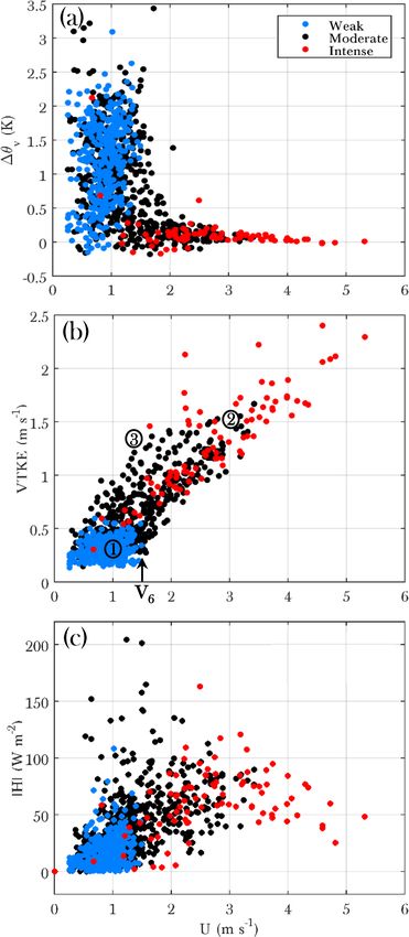
4618 J. A. Arrillaga et al.: From weak to intense downslope winds: origin and interactions
The analysis is carried out during summer, a season that the evaluation of different turbulent parameters from the EC
is characteristically very dry and warm and with nearly qui- technique. Measurements of the soil moisture are also taken.
escent large-scale conditions in central Spain, even in the For this study, measurements were carried out over an in-
mountainous areas (Durán et al., 2013). The soil is partic- tensive campaign in summer 2017 (22 June–26 September).
ularly desiccated at the end of the season, which makes it Supplementary instruments were deployed along the mast for
different from other mountainous areas in Europe such as the additional measurements, including inter alia an extra IRGA-
Pyrenees or the Alps. Summer 2017 was very warm and very SON and radiometer. Table 1 gathers specifications about the
humid (AEMET, 2017) in this region, following a very warm devices and the variables employed in this study. All the vari-
and very dry spring. In any case, it was not a particularly ables are averaged over 10 min.
rainy season and in fact, precipitation during summer 2017 Main correction and processing procedures applied to raw
took place just over a few days, so that the desiccated soil high-frequency time series are based on the software from
experienced sharp moisture increases. This sets up a strik- the EasyFlux DL programme (Campbell-Scientific, 2017),
ing working frame to explore the role of soil moisture in which provides fully corrected turbulent fluxes by applying
the surface-energy balance and the associated consequences some corrections frequently used in the related literature.
on the intensity and nature of downslope flows. And finally, The EasyFlux postprocessing software shows high correla-
the area surrounding the station is located in a relatively flat tion with the extensively used EddyPro software (Zhou et al.,
area (its slope angle is of around 2◦ ) close to the Sierra de 2018). Despiking of the high-frequency time series is carried
Guadarrama (see Fig. 1b), which allows the formation of out using diverse diagnostic codes and signal strengths. Tur-
strong surface thermal inversions. These inversions are spo- bulent parameters inferred from IRGASON measurements
radically eroded by the drained downslope flows, providing were discarded when the signal strength was below 0.9, as-
an interesting scenario for the investigation of the distinct sociated mostly with high values of the relative humidity
SBL regimes. and/or precipitation. Nevertheless, that situation was rarely
Regarding the vegetation and land use, the observational observed within the analysed database, since the algorithm
site is placed in a pasture grassland with scattered 3–5 m high employed and described in the following section ensures fair-
shrubs and small trees, and the soil is composed of granite weather conditions. Frequency corrections are applied by us-
and gneiss. At around 2 km towards the SW, a broadleaved ing transfer functions for block averaging (Kaimal et al.,
deciduous forest is found, and at the same distance to the 1989). An averaging time of 10 min was fixed for the calcu-
NW, approximately where the steep slope starts, there is lation of turbulent parameters, which is considered standard
a mixture of needleleaf evergreen (coniferous) tree cover for micrometeorological datasets (Mauritsen and Svensson,
and mosaic-tree and herbaceous cover. During nighttime, the 2007) and appropriate during the afternoon and evening tran-
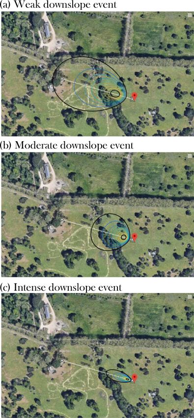
footprint of the fluxes measured at 8 m lies broadly within sition of the ABL. The election of the averaging window was
the fetch of the surrounding area. Nevertheless, the esti- supported by multi-resolution flux decomposition analyses
mated footprint area can increase horizontally up to 150– for few representative events (not shown). On the other hand,
200 m under very stable conditions associated with the weak- the double-rotation method was applied to the sonic coordi-
est downslope flows, inducing additional input from fur- nate system (Kaimal and Finnigan, 1994), so that errors in
ther inhomogeneities, although their contribution is gener- the measurement of the turbulent parameters associated with
ally small. An analysis of the calculated flux footprint for alignment issues were corrected. Other data-quality control
three representative distinct downslope events is provided in checks include moisture corrections to the sonic tempera-
Appendix A. ture following Schotanus et al. (1983) to derive the air tem-
perature and sensible heat flux, and air-density fluctuations
2.2 Data: meteorological observations and were corrected by applying the Webb, Pearman and Leun-
post-processing ing (WPL) correction (Webb et al., 1980) to water-vapour
and CO2 turbulent fluxes. Additional minor corrections and
Standard meteorological measurements and eddy-covariance quality-control checks are described in Campbell-Scientific
(EC) fluxes are recorded in the 10 m high fixed tower in (2017). Apart from those procedures, some other manual
La Herrería. The La Herrería tower is part of the Guadar- checks were considered. The results from the EasyFlux soft-
rama Monitoring Network (GuMNet, 2018), which aims at ware were compared with the results obtained with our own
providing observational meteorological and climatological programmes, which also apply various postprocessing proce-
records to deepen scientific research in the mountainous area dures. These include quality-control checks and the rotation
of Sierra de Guadarrama (Durán et al., 2018). Data from as- of the sonic-anemometer axes, among others. The compari-
pirated thermometers, cup anemometers, radiometers, a wind son showed high correlation and very good agreement.
vane and IRGASON devices, among others, are recorded
along the mast. From the IRGASON equipment, the three
components of the wind, temperature and CO2 measure-
ments are obtained at high frequency (10 Hz), which allows
Atmos. Chem. Phys., 19, 4615–4635, 2019 www.atmos-chem-phys.net/19/4615/2019/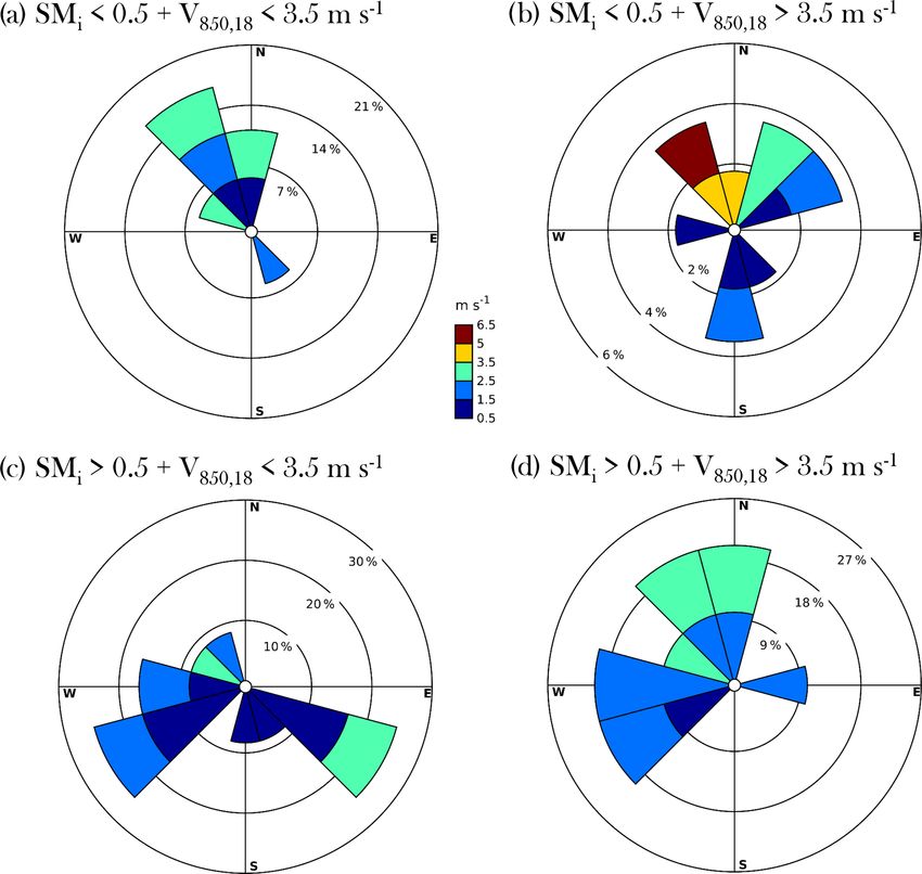
J. A. Arrillaga et al.: From weak to intense downslope winds: origin and interactions                                           4619

Table 1. Specifications about the variables measured and the devices employed in this study over the intensive summer 2017 campaign
(22 June–26 September).

           Variable                      Height (m a.g.l.)   Sampling rate     Instrument                  Model
           Air temperature                        3, 6, 10   1 Hz              Aspirated thermometer       Young 41342
           Relative humidity                             2   1 Hz              T/RH probe                  Rotronic HC2-S3
           Wind speed                             3, 6, 10   1 Hz              Cup anemometer              Vector A100LK
           Wind direction                               10   1 Hz              Wind vane                   Vector W200P
           Turbulent parameters                       4, 8   10 Hz             IRGASON                     Campbell
           Rain                                   Surface    –                 Pluviometer                 OTT Pluvio2
           Soil moisture                           −0.04     10 min            Reflectometer               CS655
           Radiation components                       1, 2   1 Hz              Four-component radiometer   Hukseflux NR01
           CO2 concentration                          4, 8   10 Hz             IRGASON                     Campbell
           Water-vapour concentration                 4, 8   10 Hz             IRGASON                     Campbell

2.3   Method: downslope-detection criteria                               The downslope flow usually lasts until sunrise, when a
                                                                      strong veering of the wind direction occurs. However, in this
The systematic and objective algorithm developed in Arril-            study, we just focus on the first stage of these flows, since
laga et al. (2018) to detect sea-breeze events, and adapted to        the main objective is to investigate their connection with the
select mountain-breeze occurrences in three different areas           onset of the SBL (defined as when the sensible heat flux, H ,
in Román-Cascón et al. (2019), is used here. We adjust the            turns negative) and the different regimes associated. During
algorithm for selecting events that fulfil predefined thermally       the summer months, the onset of the downslope flow takes
induced downslope criteria, i.e. when a shift of the wind di-         place usually before sunset, around 18:00 UTC, but it can be
rection is observed from the upslope to the downslope direc-          considerably advanced or delayed depending on a number of
tion during the afternoon and evening transition, and always          factors, which are investigated in Sect. 3.2. A wide variabil-
under a weak synoptic forcing. In this way, we evaluate the           ity in the onset time of the katabatic flow was also reported in
characteristics and impacts of the downslope flows in a more          previous studies (Papadopoulos and Helmis, 1999; Pardyjak
robust and objective way. Besides, the algorithm defines a            et al., 2009; Nadeau et al., 2013).
benchmark which is the onset of the flow, enabling the clus-             We identify the onset of the downslope flow as the first
tering of different events and their analysis in a consistent         value within the 2 h range of continuous downslope direc-
way.                                                                  tion. Having that onset time as a reference, we explore the
   The algorithm consists of four different filters, which are        characteristics and nature of downslope flows, their interac-
shown in Table 2. The first three are coincident with the             tion with turbulence and the impact on CO2 concentrations
algorithm defined in Arrillaga et al. (2018), just modifying          in the next sections.
the precipitation-amount threshold for Filter 3: 0.5 instead of
0.1 mm day−1 , since weak and scattered showers (< 0.5 mm)
                                                                      3      Characteristics of the downslope flows
do not alter the onset and development of downslope flows.
From detailed individual analysis, we found that the large-           A total of 40 thermally driven downslope wind events were
scale conditions favourable for the formation of thermally            selected from the analysed period (94 days in total). The al-
driven downslope flows are those that apply for sea breezes,          gorithm is very rigorous to ensure that the selected events are
i.e. quiescent synoptic forcing and not having the passage            mainly thermally driven downslope flows, since we just focus
of synoptic fronts (Filters 1 and 2, respectively). This fact         on the days with a weak large-scale wind in which there is a
supports the strong value of this method. The last filter (Fil-       shift from the daytime upslope to the nighttime downslope
ter 4) is based on specific criteria for downslope flows in           wind direction. The results presented hereinafter are related
La Herrería and was defined after a thorough inspection of            to these 40 downslope events.
the wind behaviour around sunset on days passing the first
three filters. An event is selected as “downslope” when wind          3.1     Wind direction and intensity
direction at 10 m is roughly perpendicular to the mountain-
range axis (see Fig. 1a), i.e. within the range 250–340◦ , for at     Figure 2 shows the direction and intensity of the selected
least 2 h at a time between 16:00 and 00:00 UTC (18:00 and            events over the 2 h period subsequent to the onset of the
02:00 LT, respectively). With this filter, events mainly driven       downslope flow. The mean downslope direction is around
by down-basin flows (from the NE) are rejected. In any case,          295◦ and the variation around this direction is small; the
downslope events are occasionally, and during short periods,          largest oscillations in the direction are observed for weak
interrupted by down-basin winds.                                      intensities. Within the database of the 40 events, we find

www.atmos-chem-phys.net/19/4615/2019/                                                       Atmos. Chem. Phys., 19, 4615–4635, 2019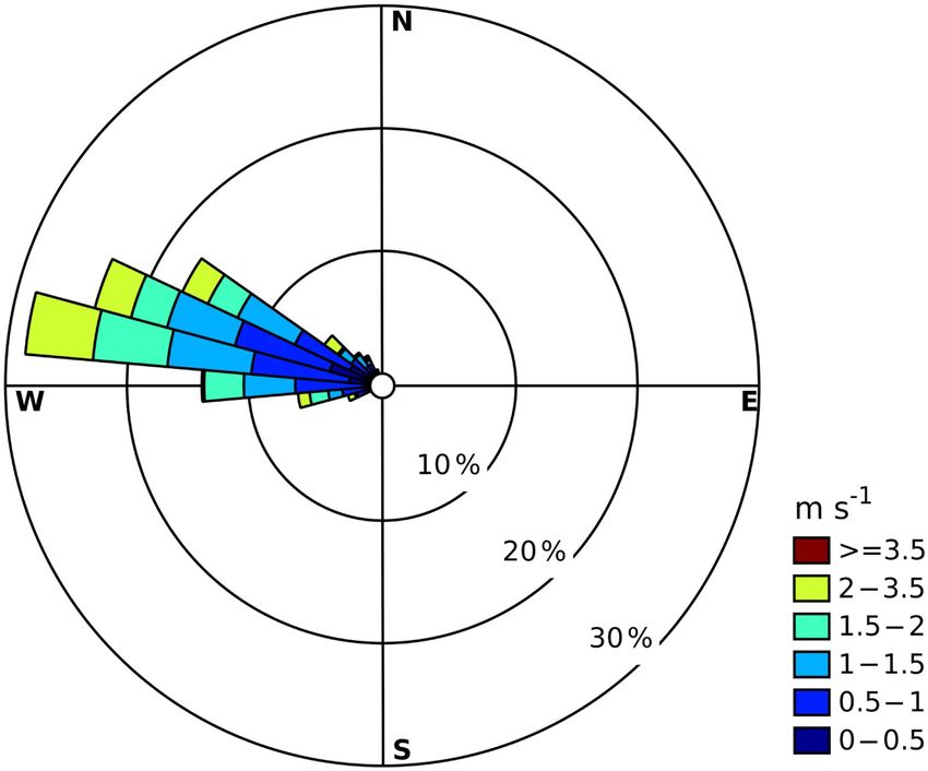
4620                                       J. A. Arrillaga et al.: From weak to intense downslope winds: origin and interactions

Table 2. Algorithm for thermally driven downslope criteria. First column indicates the filter number; second column shows the physical
description of the filter; third column lists the criteria to be fulfilled in order to pass each of the filters.

                                  Filter   Criteria                              Description
                                  1        Weak large-scale winds                V850 < 6 m s−1
                                  2        Days without synoptic cold fronts     (1θe,850 /1t) > −1.5 ◦ C / 6 h
                                  3        Non-rainy events                      pp < 0.5 mm day−1
                                  4        Minimum persistence in                WD  [250–340◦ ]2 h
                                           the downslope direction

diverse cases depending on the maximum intensity of the
downslope flow. We present in Fig. 3 the vertical profile of
the wind speed at the time of the downslope onset (Fig. 3a)
and when the intensity of the flow is maximum at 6 m
(Fig. 3b) by using box plots, which contain information about
the frequency distribution at each observational level (3, 6
and 10 m). At the time of the onset, the downslope flow is
weak at all levels (Fig. 3a); for instance, the median at 10 m
is slightly over 1 m s−1 . It can be noted that the median at 3 m
is similar to that at 6 m, and the first quartile is even smaller
at 6 m. This occurs because in some events prior to the iden-
tified onset at 10 m a very shallow katabatic or a skin flow
is usually developed and is only reflected at 3 m. This skin
flow (also denominated katabatic flow, as, for instance, in Ol-
droyd et al., 2016) can be observed when turbulence is very
weak and thermal stratification is very stable (Mahrt et al.,
2001; Soler et al., 2002; Román-Cascón et al., 2015) and oc-                Figure 2. Wind rose at 6 m over the 2 h after the onset of the downs-
casionally gives rise to a greater wind speed at 3 than at 6 m              lope flow for the 40 selected events.
and a few times even greater than at 10 m. However, when
the downslope flow is more intense, wind speed increases
                                                                            events are classified hereinafter as intense downslope events,
with height within the 10 m layer from the surface (for in-
                                                                            and they all meet the criteria that the maximum 10 min wind
stance, note that the third quartile is greater at 6 than at 3 m).
                                                                            speed at 6 m is greater than 3.5 m s−1 . It must be noted that
A maximum jet is probably found above 10 m, in accordance
                                                                            this threshold is not very high, but in the context of a weak
with the definition of downslope flow given in Oldroyd et al.
                                                                            synoptic forcing and comparing to the rest of the events, we
(2016), but we do not have the measurements to check it.
                                                                            can consider them to be relatively intense. Secondly, in some
    From Fig. 3b, the intensity distribution at all levels can also
                                                                            events, turbulence is very weak and the surface-based ther-
be observed, but in this case when the maximum 6 m wind
                                                                            mal inversion is not eroded (u∗ < 0.1 m s−1 mostly). They
speed is recorded. We find in this case that the distribution
                                                                            all occur when wind speed is very weak, and hence we clas-
above the median is elongated at all levels. In fact, the level
                                                                            sify as weak events (14 in total) those in which the maximum
of 6 m is employed to classify downslope events according
                                                                            wind speed at 6 m is below 1.5 m s−1 . The characteristics of
to their maximum intensity and the associated erosion of the
                                                                            these weak downslope flows conform with the definition of
surface-based thermal inversion. The reasons for employing
                                                                            pure thermally driven downslope or katabatic flows, as de-
the level of 6 m are outlined below. Firstly, red crosses pin-
                                                                            fined in Oldroyd et al. (2016) or Grachev et al. (2016). Fi-
point an event identified as an outlier due to its high intensity
                                                                            nally, the cases in which the maximum wind speed at 6 m is
at all levels (e.g. U > 6 m s−1 at 10 m). Together with the
                                                                            between 1.5 and 3.5 m s−1 are classified as moderate downs-
wind maximum, the surface thermal inversion is very weak
                                                                            lope flows (23 in total). A summary of the classification is
or non-existent, and the maximum of turbulence measured
                                                                            shown in Table 3. At the levels of 3 and 10 m, the events
from the turbulent kinetic energy (TKE = [(1/2)(u0 2 + v 0 2 +              showing different features cannot be so clearly detached, and
w0 2 )](1/2) ) and friction velocity (u∗ = [(u0 w 0 )2 +(v 0 w0 )2 ]1/4 )   therefore the level of 6 m is employed for the classification.
is even greater than the daytime maximum of the typical diur-               Flocas et al. (1998), for instance, studied katabatic flows at
nal cycle (generally u∗,max ' 0.5–0.7 m s−1 ). We find in ad-               a similar height (7 m), since the influence of the large-scale
dition two other events with the above-mentioned features                   wind was minimised at this level.
which are included within the right whisker. These three

Atmos. Chem. Phys., 19, 4615–4635, 2019                                                        www.atmos-chem-phys.net/19/4615/2019/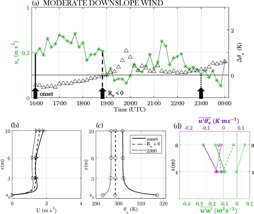
J. A. Arrillaga et al.: From weak to intense downslope winds: origin and interactions                                                      4621

                                                                         Figure 4. Histograms of the difference between the downslope on-
                                                                         set time and sunset time, for the three groups of intensities (bars)
                                                                         and for different static stabilities at the moment of the onset (lines).
                                                                         Values of the net radiation (Rn ) and turbulent kinetic energy (TKE)
                                                                         are also indicated on both sides from the −1.5 h time difference.

                                                                         3.2   Factors influencing intensity
Figure 3. Box plots of the wind-speed profile at 3, 6 and 10 m for the
downslope events, (a) at the time of the onset and (b) at the time of    Once the downslope events are classified according to their
the maximum value at 6 m (from the onset to 00:00 UTC) for each          maximum intensity, we first explore the factors that induce
event. The red vertical line within blue boxes represents the median,    different intensities. Figure 4 shows a histogram with the
the blue box delimits first and third quartiles, and whiskers delimit    difference between the onset time of the downslope flow
the most extreme points not considered outliers (red crosses). Black     and sunset time (it ranges from 18:10 UTC in September to
vertical lines and arrows pinpoint the limits for the wind speed at      19:40 UTC in June), for different intensities in colours, and
6 m that separate weak, moderate and intense downslope events.           in lines for a different static stability of the thermal profile at
                                                                         the moment of the onset. Values of the net radiation (Rn ) and
Table 3. Classification of the downslope events according to their       TKE are also indicated. The static stability was estimated by
maximum 10 min averaged wind speed at 6 m from the onset to              fitting the virtual potential temperature at the different ver-
00:00 UTC.                                                               tical levels (surface, 3, 6 and 10 m) to a logarithmic profile,
                                                                         as explained in detail in Appendix B. Virtual potential tem-
     Type          Definition                          Number
                                                      of events
                                                                         perature was calculated using measurements from aspirated
                                                                         thermometers and a T/RH probe (see Table 1). The skin tem-
     Weak          Umax < 1.5 m s−1                          14          perature was calculated from the upward longwave radiation
     Moderate      1.5 m s−1 ≤ Umax ≤ 3.5 m s−1              23          by employing the Stefan–Boltzmann law.
     Intense       Umax > 3.5 m s−1                           3              From the classification introduced in Appendix B, we in-
                                                                         fer the relationship between the earlier or later onset of the
                                                                         downslope wind, turbulence and the associated thermal strat-
   This classification is employed in the following sections             ification at the moment of its onset, and the intensity of
to better illustrate the differences between the downslope               the flow. On the one hand, intense downslope flows develop
events, their formation and development mechanisms, and                  when the onset takes place prior to 1.5 h before sunset, the
the very distinct way in which they interact with local tur-             stratification within the first 10 m is still unstable, and Rn
bulence (in particular this is addressed in Sects. 4 and 5).             and TKE are always greater than 80 W m−2 and 0.8 m2 s−2 ,
                                                                         respectively. On the other hand, weak downslope or katabatic
                                                                         flows occur when the onset takes place later than 1.5 h before
                                                                         sunset and with neutral or stable stratification. In this case,
                                                                         TKE is almost an order of magnitude smaller (on the order

www.atmos-chem-phys.net/19/4615/2019/                                                       Atmos. Chem. Phys., 19, 4615–4635, 2019
4622                                    J. A. Arrillaga et al.: From weak to intense downslope winds: origin and interactions

                                                                       reanalysis wind speed employed in the selection algorithm,
                                                                       by choosing the grid point at 850 hPa closest to La Herrería
                                                                       (40.5◦ N, 4◦ W) at 18:00 UTC. At that point, the 850 hPa
                                                                       level is approximately at 800 m above ground level (a.g.l.),
                                                                       sufficiently close to the surface to be representative of the
                                                                       synoptic wind at the surface level and far enough to be out of
                                                                       the influence of downslope winds.
                                                                          We find that intense downslope flows (orange-reddish) de-
                                                                       velop when the soil is drier and the large-scale wind is weak
                                                                       and blowing from the N–NW (Fig. 5b). This direction is per-
                                                                       pendicular to the mountain range axis (Fig. 1a) and approx-
                                                                       imately coincident with the downslope direction (Fig. 5).
                                                                       However, under those conditions, we find weak downslope
                                                                       or katabatic flows (dark blue) when the large-scale wind
                                                                       blows from parallel or opposite directions (S or E–NE, for
                                                                       instance), although most of the katabatics occur mainly when
                                                                       the soil is moister and the synoptic forcing is very weak
                                                                       (Fig. 5c). Katabatic flows establish primarily for W–SW and
                                                                       S–SE large-scale winds, but they can also occur for N–NW
                                                                       winds when their intensity is very weak (Fig. 5a). Overall,
Figure 5. Wind roses representing the maximum downslope wind           the intensity of downslope winds increases with decreasing
speed at 6 m in colours, for different directions from the National
                                                                       soil moisture and increasing synoptic forcing with a N–NW
Centers for Environmental Prediction (NCEP) reanalysis wind at
850 hPa, at the closest grid point from La Herrería (40.5◦ N, 4◦ W)
                                                                       direction.
at 18:00 UTC. Wind roses are shown for different values of the soil-      The role of the soil moisture in the surface energy balance
moisture index (SMi ) and the reanalysis wind speed (V850,18 ) (a–     is in general complex. The longwave-radiative loss and soil-
d). Note that the frequency scale of the wind roses is variable.       heat flux show a peak when the relative desiccation of the
                                                                       soil is large (not shown). However, after precipitation has oc-
                                                                       curred, soil moisture increases considerably and the cooling
of or smaller than 0.1 m2 s−2 ), and Rn < 40 W m−2 always;             of the soil can also be enhanced. This bimodal behaviour is
it is in fact negative in more than 80 % of the cases. Moderate        in any case vague and ambiguous, and it must be supported
downslope flows, however, occur either when the onset takes            by more conclusive observational results.
place earlier or later, and hence independently of turbulence             Overall, we find that the combination of low soil moisture,
and the associated thermal stratification.                             which enhances the thermal forcing, and the synoptic wind
    This result suggests the existence of external factors affect-     direction coincident with the downslope direction (N–NW),
ing the earlier or later onset of downslope winds. Particularly,       adding an important dynamical contribution, induces an ear-
we focus on the soil moisture and the large-scale wind.                lier onset of downslope flows. The onset occurs when strati-
    To explore the influence of soil moisture, we define an in-        fication is still unstable and convective turbulence relatively
dex that provides a measure of the relative desiccation of             strong, which enables the development of intense downslope
the soil over the summer. This soil-moisture index is de-              flows. If those conditions are not met, the onset occurs later
fined as the ratio between the observed liquid water vol-              when stratification is already neutral or stable, which lim-
ume and the maximum value throughout the analysed period               its the intensification of downslope flows. To understand the
(0.14 m3 m−3 ): SMi = SM/SMmax . We separate the events                evolution of downslope flows after their onset, we explore
into drier (SMi ≤ 0.5) and moister (SMi > 0.5) cases. On the           their interaction with turbulence in the next subsection.
other hand, to explore the influence of the large-scale wind
(V850,18 : at 850 hPa at 18:00 UTC), we separate the downs-            3.3   Interconnection between downslope flows and
lope events into very weak (V850,18 ≤ 3.5 m s−1 ) and weak                   turbulence
(V850,18 > 3.5 m s−1 ) synoptic forcing.
    The influence of the large-scale wind speed and direction,         Thermal stratification and the associated turbulence at the
and soil moisture, are investigated in Fig. 5. The maximum             moment of the onset modulate the intensity and subsequent
downslope intensity at 6 m together with the direction of              development of the downslope flow. If the downslope flow
the synoptic wind are represented in wind-rose form for the            arrives when the stratification is still unstable and the sur-
above-mentioned drier (Fig. 5a, b) and moister (Fig. 5c, d)            face thermal inversion (hereinafter measured from 1θv ) is
cases, and for a very weak (Fig. 5a, c) and weak (Fig. 5b,             not formed yet, the downslope flow strengthens progres-
d) synoptic forcing. The synoptic wind is estimated from               sively. Later, due to the radiative energy loss (Rn < 0), the
the National Centers for Environmental Prediction (NCEP)               stable stratification is already established (1θv > 0), and the

Atmos. Chem. Phys., 19, 4615–4635, 2019                                                 www.atmos-chem-phys.net/19/4615/2019/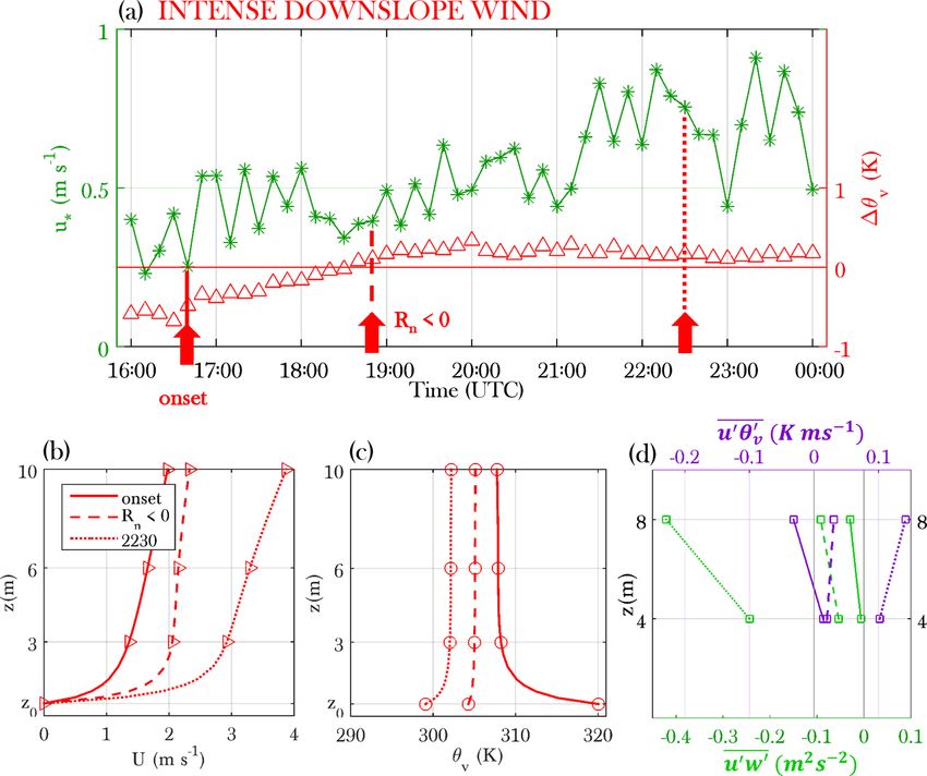
J. A. Arrillaga et al.: From weak to intense downslope winds: origin and interactions                                               4623

katabatic (thermal) contribution of the downslope flow is en-
hanced. Given that the wind shear associated with the downs-
lope flow is already high, the negative H strengthens (H < 0)
and after a while compensates the energy loss at the sur-
face, impeding the development of the surface-based ther-
mal inversion and inducing near-neutral stability conditions
(Van de Wiel et al., 2012a). In that way, intense downs-
lope flows give rise to a WSBL. On the other hand, with-
out a clear dynamical contribution of the large-scale flow,
the downslope flow is established later, when negative buoy-
ancy of the air adjacent to the surface enhances the katabatic
input. However, this katabatic flow is not intense enough
to increase turbulent mixing substantially. Besides, the in-
crease of the downslope intensity and the associated wind
shear are limited by the stable stratification itself. Thus, even
the maximum sustainable heat flux does not compensate the
radiative energy loss. Consequently, the bottom of the SBL
cools down, which contributes to enhance the stable stratifi-
cation. This positive feedback occurring under weak downs-
lope flows suppresses turbulence and gives rise to a VSBL
(Van de Wiel et al., 2012b). For moderate downslope flows,
any of the two regimes can occur depending on the onset time
and the dynamical contribution of the large-scale flow. These
mechanisms are explored in the following sections.
   Figure 6 shows the temperature stratification 1θv = θv
(10 m) – θv (3 m), the turbulence velocity scale VTKE and H
with respect to U at 6 m. VTKE is calculated as the square
root of the TKE. We just represent the 10 min average values
in which the wind direction is downslope (until 00:00 UTC)
and H is negative, so that the downslope flow is present (for
instance, not the down-basin wind) and the SBL is already
established. By representing 1θv vs. U , we find a contrasting
relationship for weak and intense downslope flows (Fig. 6a).
Katabatic flows give rise to a strongly stratified SBL (1θv
up to 2 K), whereas intense downslope flows are linked with
very weak or almost non-existent surface-based thermal in-
versions. Interestingly, for a few 10 min values with sim-
ilar wind speed (U ' 1–1.5 m s−1 ), the thermal stratifica-
tion is very different between weak and intense downslope
flows, which suggests the existence of distinct regimes in          Figure 6. (a) Thermal stratification (1θv = θv (10 m) − θv (3 m)),
the SBL. On the other hand, we find for very weak wind              (b) turbulence velocity scale (VTKE ) and (c) the absolute value of
speed (U < 1 m s−1 ) a large variability of thermal stratifica-     the sensible heat flux (H ) at 8 m vs. wind speed (U ) at 6 m. The
tion, that occurs because around the onset of the downslope         numbers in panel (b) pinpoint the SBL regimes defined in Sun et al.
flow the thermal inversion is still absent or very weak in most     (2012): (1) weak turbulence driven by local instabilities, (2) intense
                                                                    turbulence driven by the bulk shear and (3) moderate turbulence
of the cases. At the upper limit, however, 1θv tends to zero
                                                                    driven by top-down events. The threshold wind speed (V6 ) at which
when wind speed increases its value. Moderate downslope
                                                                    the HOST transition occurs is indicated too.
flows show both types of behaviour, with the transition tak-
ing place for U ' 1.5 m s−1 .
   By representing the turbulence strength VTKE vs. U at 6 m,
we confirm the sharp transition for U = 1.5 m s−1 (Fig. 6b).        and defined as the HOckey-Stick Transition (HOST) in
Katabatic flows are associated with very weak turbulence            Sun et al. (2015). They identified three turbulence regimes in
(VTKE < 0.5 m s−1 ) that hardly increases with wind speed,          the SBL depending on the relationship between turbulence
while turbulence for intense downslope flows is consider-           and wind speed. In Regime 1, turbulence is very weak and
ably greater and increases approximately at a linear rate with      generated by local shear; in Regime 2, turbulence is strong
U . This behaviour was first observed in Sun et al. (2012)          and generated by the bulk shear U/z (hence the linear re-

www.atmos-chem-phys.net/19/4615/2019/                                                 Atmos. Chem. Phys., 19, 4615–4635, 2019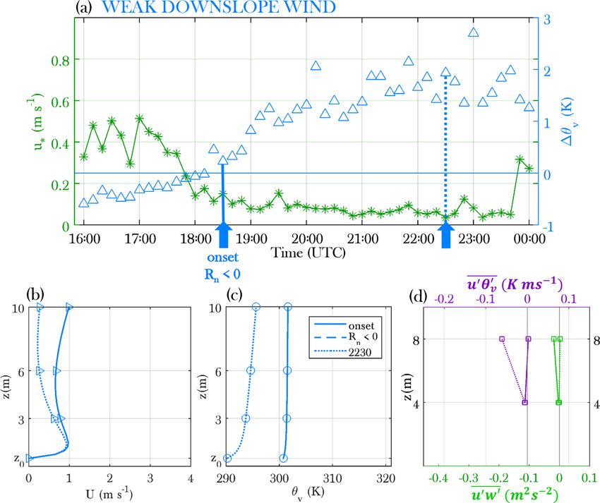
4624                                 J. A. Arrillaga et al.: From weak to intense downslope winds: origin and interactions

lationship with wind speed); and finally, in Regime 3, tur-       and this day the synoptic situation was also characterised by
bulence is moderate and mainly generated by top-down tur-         the Azores High, but in this case with a weak NE forcing,
bulent events. The three regimes are pinpointed in Fig. 6b.       coinciding with the direction of the down-basin winds in the
The threshold value for the wind speed depends on height          basin in which La Herrería is located. Besides, the soil mois-
and sets the value above which the abrupt transition from         ture was low. This event was marked by the interaction be-
Regime 1 to Regime 2 occurs. Since in our case z = 6 m, it        tween local downslope and down-basin winds. Finally, the
is indicated as V6 in the figure. Katabatics are clearly asso-    intense event is 27 July, again marked by the Azores High,
ciated with Regime 1 and intense downslope flows, instead,        but with a weak NW forcing coinciding with the direction
with Regime 2. Moderate downslope flows can give rise to          of downslope flows, adding a dynamical input to the local
either of the three regimes. We just show the relationship for    flow. Soil moisture was also low for this case. In addition to
z = 6 m, and HOST in our case occurs for V6 = 1.5 m s−1 ,         the strong turbulence associated with the intense downslope
which is significantly lower than the value at that height from   flow, this event is chosen due to its particular influence on the
Sun et al. (2012) (' 3 m s−1 ) over relatively flat and homo-     CO2 transport, which is addressed in Sect. 5.
geneous terrain (Poulos et al., 2002). This lower threshold
could be partly induced by the proximity of the jet maxi-         4.1   Origin and underlying physical mechanisms
mum, as, for instance, is shown in Fig. 8. Besides, V6 co-
incides with the threshold value we anticipated for defining      In previous sections, we have shown that external factors
katabatic flows (Table 3). We measure a slope of ∼ 0.5 for        such as soil moisture and the synoptic wind modulate the in-
VTKE vs. U for Regime 2, while it is ∼ 0.25 in the results        tensity of downslope winds, which is at the same time linked
from Sun et al. (2012).                                           with an earlier or later onset time. In order to understand the
   In Fig. 6c, we explore how downslope intensities and           physical processes underlying the formation and subsequent
turbulence strength are manifested in terms of heat flux.         evolution of the downslope flows, the momentum and heat
The downward H , i.e. when the SBL is already established         budgets for the three individual events are explored following
(H < 0), is represented in absolute values. The smallest H        the two-dimensional simplified equations from Manins and
values are observed for katabatic flows, when U < 1 m s−1 .       Sawford (1979), which were employed in the recent stud-
The highest values take place for moderate downslope flows        ies from Nadeau et al. (2013) and Jensen et al. (2017). The
when U lies between 1.5 and 2.5 m s−1 . We find a few data        slope-parallel momentum and heat budgets are, respectively,
from some intense downslope flows in which H is nearly            given by
zero for that wind-speed range, when the thermal inversion
                                                                  ∂u   ∂u    ∂u gd sin α ∂u0 w0 1 ∂(p − pa )
has just been formed. For intense downslope winds, the peak          +u +w       −       +     +             = 0,
is reached at U ' 3 m s−1 , and above that intensity H de-        ∂t   ∂s    ∂n      θva    ∂n   ρ   ∂s
creases, since it is limited by the neutral stratification.       (I) (II) (III)   (IV)    (V)      (VI)      (1)
   So far, we have explored all the selected downslope events
together and learnt about their main characteristics, influ-
encing factors and connection with the SBL regimes. We            ∂θv    ∂θv    ∂θv ∂w0 θv 0    1 ∂Rn
                                                                      +u     +w    +         +        = 0,
have observed how the turbulent characteristics of the ABL        ∂t     ∂s     ∂n   ∂n        ρcp ∂n
and the nocturnal regime can be predicted from the intensity      (I)      (II)    (III)    (IV)          (V),                 (2)
of the downslope flow at 6 m. However, in order to better
understand the mechanisms underlying their formation, de-         where s and n are the slope-parallel and slope-normal coor-
velopment and their complex interaction with turbulence in        dinates in accordance with the double-rotation of the axes; t
the SBL, we target the analysis of individual representative      is time. u is the streamwise wind, w the slope-normal wind,
events.                                                           d = θv − θva is the temperature deficit defined as the differ-
                                                                  ence between the perturbed virtual potential temperature and
                                                                  the unperturbed potential temperature, α (' 2◦ ) is the slope
4   Analysis of representative downslope events                   angle, g = (9.81 m2 s−2 ) gravity acceleration, ρ the air den-
                                                                  sity, p is the measured local pressure, pa the ambient pres-
We choose representative weak, moderate and intense               sure field and cp (= 1005 J kg−1 K−1 ) the specific heat of the
downslope events, so that their contrasting features and dis-     air at constant pressure. The bar is used for indicating 10 min
tinct influencing mechanisms are revealed. The weak downs-        time averaging, and the primes indicate a perturbation from
lope event is 13 August and is characterised by the presence      the temporal mean.
of a katabatic flow and a VSBL. In short, the synoptic sit-          Term I in Eq. (1) represents momentum storage, terms
uation was marked by the Azores High and a thermal low            II and III represent horizontal and vertical advection, re-
over the Iberian Peninsula inducing a weak S flow, which          spectively, term IV is buoyancy acceleration, term V the
was related to a weaker downslope intensity in Fig. 5. The        momentum-turbulent-flux divergence and term VI represents
SMi was high for this case. The moderate event is 25 July,        the along-slope pressure gradient. Regarding the heat-budget

Atmos. Chem. Phys., 19, 4615–4635, 2019                                            www.atmos-chem-phys.net/19/4615/2019/
J. A. Arrillaga et al.: From weak to intense downslope winds: origin and interactions 4625
equation (Eq. 2), term I is the heat storage, terms II and III 00:00 UTC (which can be observed in Fig. 8a). It produces an
horizontal and vertical advection, respectively, term IV the upward momentum transport from the skin flow and a sud-
kinematic-heat-flux divergence and the last term represents den warming due to turbulent mixing, demonstrating that the
Rn divergence. For the calculation of d, the difference be- very stable regime may be occasionally interrupted.
tween the levels of 2 and 20 m is calculated (as in Jensen The onset of the moderate downslope event (Fig. 7c and d)
et al., 2017). For that, the values are obtained from the ver- takes place rather earlier. According to the momentum bud-
tical extrapolation from the fit to the logarithmic profile (see get, either advection or the along-slope pressure gradient, or
Eq. B1). All derivatives are evaluated using forward finite both, are responsible for the intensification of the downslope
differences, between the levels of 4 and 8 m in term V in flow when the buoyancy acceleration is still negative. When
Eq. (1) and term IV in Eq. (2), and between the levels of 1 and Rn turns negative, the down-basin wind arrives, and due to
2 m in term V in Eq. (2). On the other hand, the terms with the collision between both, turbulence decreases and the fur-
slope-parallel gradients are considered residuals of the equa- ther intensification of the downslope flow is prevented. Due
tions due to the lack of additional spatial measurements, and to the interaction between the down-basin wind (NE) and the
vertical advection in both equations (term III) is null (w = 0) downslope flow (NW), turbulence is intermittent and of vari-
due to the imposition from the double-rotation method. For able intensity, and the momentum balance is marked by the
this, 10 min averages are used. oscillating equilibrium between the momentum-flux diver-
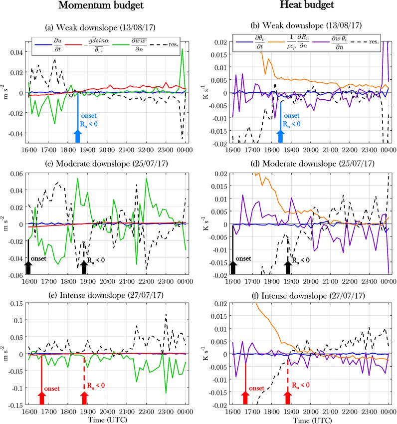
The times series of these terms are represented and com- gence and the advective and pressure-gradient terms. Regard-
pared in Fig. 7 for the representative weak, moderate and in- ing the heat budget, the main source of cooling is advection,
tense downslope events, from 16:00 to 00:00 UTC. Due to even after Rn turns negative. After 20:00 UTC, however, the
the lack of spatial gradients, the estimation of the residual advection produces warming and compensates the cooling
has some uncertainty in particular for the momentum budget, from the heat-flux divergence.
since there are two terms within the residual of Eq. (1) and During the intense event (Fig. 7e and f), the governing
only one in Eq. (2). In any case, the comparison between the forcing in driving the intensification of the downslope flow
three events explains the differences in the physical mecha- is dynamical: either or both advective and large-scale pres-
nisms underlying the formation and development of the dis- sure terms dominate over the local buoyancy acceleration
tinct downslope flows. While the vertical axis for the heat and are balanced by the turbulent-flux divergence. Given that
budget is kept constant and is limited to 0.02 K s−1 for better the slope of the nearby mountain towards the NW is steep
showing the differences, it is variable for the momentum bud- (' 25◦ ), and with an enhanced temperature deficit due to
get due to the highly distinct relative weight of the different the greater desiccation of the soil, the buoyancy-acceleration
terms. term is considerably greater over the slope than in La Her-
Prior to the onset of the weak downslope flow (Fig. 7a rería. Furthermore, the mountain-range axis is directed SW–
and b), the bottom of the surface layer cools down, driven NE, so that sunset takes place at the back of it. Therefore, the
mainly by the kinematic-heat-flux divergence, as observed cooling starts earlier along the slope than in La Herrería. The
in the analysis from Jensen et al. (2017), whereas momen- heat budget shows that before Rn turns negative, the source
tum is produced by the turbulent-flux divergence. This sug- of cooling is advection from the slope, compensating the ra-
gests the formation of a very shallow flow below the lowest diative heating. These findings confirm that the origin of the
observational level before the recorded onset. After the on- early flow is the advected cold drainage front from the nearby
set, the main source of momentum is buoyancy acceleration, steep slope. Later, the main sources of cooling are the heat-
driven by the local surface cooling, in principle balanced by flux divergence and the radiative divergence from 21:00 UTC
large-scale pressure and advective terms. This mechanism on, which are compensated by the warm advection. In any
conforms also with the findings from Nadeau et al. (2013), case, the cooling from the heat-flux divergence is smaller
confirming that weak downslope winds share the character- than in the moderate event, due to the constrain from the
istics of katabatic flows. The cooling after the onset is pri- weak thermal stratification. A similar situation was reported
marily ruled by the heat-flux divergence, compensated by the in Papadopoulos and Helmis (1999), where the flow reached
heating produced by the radiative divergence. Despite the ra- the foot of the slope as a drainage front from more elevated
diometers having previously been calibrated by being com- cold-air sources, before the establishment of the thermal in-
pared at the same level, the calculation of the divergence can version. This earlier onset at the foot was observed when
be subject to errors due to the closeness (= 1 m) between the relative humidity was lower at the slope site, when the lo-
devices. Furthermore, Steeneveld et al. (2010) eliminated the cal thermal structure did not sustain katabatic motion, as in
radiative measurements coinciding with wind speed at 10 m our intense downslope event. They showed how advective
below 1.5 m s−1 , to assure that radiometers were sufficiently effects dominated in this case and the arrival of the drainage
ventilated. Hence, there might be certain uncertainty in the front produced a temperature fall. Additionally, going along
estimation of the radiative divergence, and the advective term with our findings, they observed that the growth rate of this
could be responsible for balancing the cooling otherwise. In downslope flow was more intense due to weaker ambient sta-
addition, this event shows a sudden turbulent burst at around
www.atmos-chem-phys.net/19/4615/2019/ Atmos. Chem. Phys., 19, 4615–4635, 20194626 J. A. Arrillaga et al.: From weak to intense downslope winds: origin and interactions
Figure 7. Time evolution of the different terms from the momentum (a, c, e) and heat budget (b, d, f) for the weak downslope (a, b), moderate
downslope (c, d) and intense downslope (e, f) events. The solid arrows point to the downslope onset time (with the vertical solid line) and
the time at which Rn turns negative (with the dashed vertical line).
bility, whereas the existence of a surface-based thermal inver- horizontal turbulent fluxes (Figs. 8d, 9d and 10d) are shown
sion opposed the flow progression. below at three times of interest: at the moment of the onset,
when Rn turns negative and finally at 22:30 UTC when the
4.2 Nature and interaction with turbulence SBL is already well formed. The logarithmic fitting of the
discrete observed measurements for both wind speed and θv
After inspecting the physical mechanisms underlying the dif- is also depicted in panels (b) and (c) of the respective fig-
ferent evolution of the three representative downslope events, ures. With respect to the turbulent fluxes, we can infer from
we characterise the associated wind and thermal profiles, as their sign whether the jet associated with the downslope flow
well as the interconnection of the flow with local turbulence, is located below or above the measurements (Grachev et al.,
in Figs. 8, 9 and 10, for the weak, moderate and intense 2016; Oldroyd et al., 2016). At the height of the wind-speed
downslope events, respectively. We show the time series of maximum, both turbulent fluxes become zero, and above the
thermal stratification and friction velocity at 8 m (Figs. 8a, jet u0 θv0 < 0 and u0 w0 > 0, whereas below the jet u0 θv0 > 0 and
9a and 10a). Vertical profiles of the wind speed (Figs. 8b, 9b u0 w 0 < 0.
and 10b), θv (Figs. 8c, 9c and 10c) and heat and momentum
Atmos. Chem. Phys., 19, 4615–4635, 2019 www.atmos-chem-phys.net/19/4615/2019/You can also read