Atypical VRE Variability in Power System Planning and Performance

DEGREE PROJECT IN MECHANICAL ENGINEERING,
SECOND CYCLE, 30 CREDITS
STOCKHOLM, SWEDEN 2018

Atypical VRE Variability in Power
System Planning and Performance
Illustrated by the case studies of Guinea-Bissau
and Turkey

VIRGINIA ATTJE INGRID ALBERTINE
POTTER VAN LOON

KTH ROYAL INSTITUTE OF TECHNOLOGY
SCHOOL OF INDUSTRIAL ENGINEERING AND MANAGEMENT

TRITA-ITM-EX 2018:584

iii

This master thesis research has been conducted at the Energy Sector Management Assistance
Program (ESMAP) and The World Bank Energy and Extractives Global Practice as part of the
Sustainable Energy Engineering Master of Science Program at KTH Royal Institute of Technology.

Supervisor: Debabrata Chattopadhyay (ESMAP, The World Bank)
Examiner: Francesco Fuso Nerini (KTH division of Energy System Analysis (dESA))

iv

Contents
List of Figures ......................................................................................................................................... vi
List of Tables ......................................................................................................................................... vii
List of Abbreviations ............................................................................................................................ viii
Acknowledgement ................................................................................................................................. ix
Abstract ................................................................................................................................................... x
Sammanfattning..................................................................................................................................... xi
1 Introduction .................................................................................................................................... 1
2 Background ..................................................................................................................................... 3
 2.1 Variable Renewable Energy .................................................................................................... 3
 2.1.1 VRE Generation Technologies: Wind and Solar PV ......................................................... 4
 2.2 VRE Challenges ........................................................................................................................ 5
 2.2.1 Stable, Reliable and Flexible Power Systems .................................................................. 5
 2.2.2 Challenges for Power System Actors .............................................................................. 5
 2.3 VRE Integration ....................................................................................................................... 6
 2.3.1 Contingency Planning...................................................................................................... 8
 2.4 Long-Term Power System Planning Models ........................................................................... 8
 2.4.1 High VRE Shares in Power System Planning.................................................................... 8
 2.4.2 Least Costs Power System Planning Models ................................................................... 9
 2.5 Atypical vs. Typical Variability ................................................................................................. 9
3 Country Profile: Guinea-Bissau ..................................................................................................... 11
 3.1 Socio-Economic Profile ......................................................................................................... 11
 3.2 Energy System and Resources .............................................................................................. 11
 3.3 Electricity System .................................................................................................................. 12
 3.4 Energy Policy ......................................................................................................................... 12
 3.5 Solar PV CF Variability ........................................................................................................... 12
 3.6 Case Study Guinea-Bissau ..................................................................................................... 14
4 Country Profile: Turkey ................................................................................................................. 15
 4.1 Socio-Economic Profile ......................................................................................................... 15
 4.2 Energy System and Resources .............................................................................................. 15
 4.3 Electricity System .................................................................................................................. 16
 4.4 Energy Policy ......................................................................................................................... 17
 4.5 Solar and Wind CF Variability................................................................................................ 18
 4.6 Case Study Turkey ................................................................................................................. 20
5 Methodology................................................................................................................................. 22
 5.1 Model .................................................................................................................................... 22

v

 5.1.1 Objective Function ........................................................................................................ 23
 5.1.2 Constraints and Balances .............................................................................................. 23
 5.1.3 Turkey Specific Constraints ........................................................................................... 23
 5.1.4 Including Contingency Planning for Guinea-Bissau ...................................................... 24
 5.2 Input Data ............................................................................................................................. 25
 5.2.1 Input Data: Guinea-Bissau ............................................................................................ 25
 5.2.2 Input Data: Turkey ........................................................................................................ 26
6 Results & Discussion ..................................................................................................................... 28
 6.1 Guinea-Bissau: Performance of TMY-Based Power System Design...................................... 28
 6.2 Guinea-Bissau: Power System Design with Atypical Variability............................................ 30
 6.3 Turkey: Performance of TMY-Based Power System Design ................................................. 31
 6.4 Turkey: Power System Design with Atypical Variability........................................................ 33
 6.5 Contingency Planning............................................................................................................ 35
 6.5.1 Performance of TMY-Based Power System Design with Contingency Planning........... 35
 6.5.2 Power System Design Considering Contingency Planning ............................................ 35
 6.5.3 Scenario: Solar vs. LNG with SC and variability ............................................................. 36
 6.6 Data Reduction Suggestion - Adding Years Incrementally .................................................... 38
 6.7 The Performance Analysis as Data Reduction Tool .............................................................. 39
 6.8 Methodological Limitations and Future Research ................................................................ 39
7 Conclusion ..................................................................................................................................... 41
8 Bibliography .................................................................................................................................. 43
9 Appendix ....................................................................................................................................... 48
 9.1 Turkey Demand Forecast ...................................................................................................... 48
 9.2 Guinea-Bissau: HFO+LNG scenario without contingencies .................................................. 48
 9.3 Guinea-Bissau: Solar vs. HFO with SBC and Lower Solar CAPEX ........................................... 48
 9.4 Guinea-Bissau: Feasibility of Batteries .................................................................................. 49

vi

List of Figures
Fig. 1. Global Electricity Generation (TWh) Projection 2015-2050 [1]. .................................................. 3
Fig. 2. Global Installed Capacity (GW) Projection to 2015-2050 [1]. ...................................................... 4
Fig. 3. Share of VRE in Power Mix (%)2016 [6]....................................................................................... 4
Fig. 4. Energy Consumption by Source (%)Guinea-Bissau 2015 [51]. ................................................... 11
Fig. 5. Average Annual Solar PV CF Guinea-Bissau 1994-2017. ............................................................ 13
Fig. 6. Daily Pattern Solar PV CF Average and Coefficient of Variation for Guinea-Bissau 1994 – 2017.
 .............................................................................................................................................................. 13
Fig. 7. Solar CF for Guinea-Bissau for 1994 and 2017. .......................................................................... 14
Fig. 8. Energy Consumption by Source Turkey 2015 [51]. .................................................................... 15
Fig. 9. Electricity Generation by Source Turkey 2015 [55]. ................................................................... 16
Fig. 10. Annual Profile Geothermal and Hydroelectric CF Turkey [66]. ................................................ 17
Fig. 11. Average Annual Wind CF Turkey 1994-2017. ........................................................................... 18
Fig. 12. Average Annual Solar PV CF Turkey 1994-2017. ...................................................................... 18
Fig. 13. Daily Pattern Wind CF Average and Coefficient of Variation Turkey 1994-2017. .................... 19
Fig. 14. Daily Pattern Solar PV CF Average and Coefficient of Variation Turkey 1994-2017. ............... 19
Fig. 15. Wind CF 12PM Turkey 1994 and 2017. .................................................................................... 20
Fig. 16. Solar PV CF 12PM Turkey 1994 and 2017. ............................................................................... 20
Fig. 17. Planned vs. actual solar PV generation and system cost Guinea-Bissau 2030: HFO vs. solar
scenario. ................................................................................................................................................ 29
Fig. 18. Planned vs. actual solar PV generation and system cost Guinea-Bissau 2030: LNG vs. solar
scenario. ................................................................................................................................................ 30
Fig. 19. Optimized generation mix Turkey 2027 with solar PV and wind cap. ..................................... 31
Fig. 20. Planned vs. actual solar PV generation and system cost Turkey 2027. ................................... 32
Fig. 21. Planned vs. actual wind generation and system cost Turkey 2027.......................................... 32
Fig. 22. Planned vs. actual VRE generation and unserved energy Turkey 2027. .................................. 33
Fig. 23. Planned vs. actual solar PV generation and system cost Guinea-Bissau 2030: LNG vs. solar
with solar contingency scenario. .......................................................................................................... 35
Fig. 24. Accumulated years analysis for incremental variability Guinea-Bissau 2030: LNG+SC scenario.
 .............................................................................................................................................................. 38
Fig. 25. Accumulated years analysis for variability Guinea-Bissau 2030: HFO+LNG+SC variability. ..... 39
Fig. 26. Optimized system costs with and without battery storage Guinea-Bissau 2030. ................... 50
Fig. 27. Solar PV capacity selection with and without battery storage Guinea-Bissau 2030. .............. 50

vii

List of Tables
Table 1. Generation Expansion Plan (MW) Turkey 2017-2021 [66]. .................................................... 16
Table 2. Input OPEX and CAPEX existing and potential generators in Guinea-Bissau [56]................... 25
Table 3. Emission Intensity Fossil Fuels Guinea-Bissau and Turkey [76]. ............................................. 26
Table 4. Input OPEX and CAPEX existing and potential generators in Turkey. ..................................... 26
Table 5. Summary results impact solar PV CF atypical variability Guinea-Bissau 2030. ....................... 30
Table 6. Summary results impact solar PV and wind CF atypical variability Turkey 2027. ................... 34
Table 7. Summary results impact contingency planning Guinea-Bissau 2030: HFO+LNG vs. solar
scenario. ................................................................................................................................................ 36
Table 8. Summary results LNG with SC and variability Guinea-Bissau 2030. ....................................... 37
Table 9. Summary results impact SBC and lower solar CAPEX Guinea-Bissau 2030: HFO scenario. .... 49

viii

List of Abbreviations
BStorage Battery Storage
BStorInj Battery Storage Injection
BStorOut Battery Storage Withdrawal
Cap Capacity
CAPEX Capital Expenditures
CF Capacity Factor
CV Coefficient of Variation
EAGD National Electricity and Water
EPM Electricity Planning Model
ESMAP Energy System Assistance Management Program
GAMS General Algebraic Modeling System
Gen Generation
HFO Heavy Fuel Oil
IDE Integrated Development Environment
INDCs Intended Nationally Determined Contributions
IRENA International Renewable Energy Agency
LNG Liquified Natural Gas
LP Linear Programming
OPEX Operational Expenditures
PPAs Power Purchasing Agreements
PV Photovoltaic
S Scenario with spinning reserves, which cannot be provided by batteries
SB Scenario with spinning reserves which can be provided by batteries
SBC Scenario with solar contingency planning and spinning reserves which can be
 provided by batteries
SC Scenario with solar contingency planning and spinning reserves with cannot be
 provided by batteries
SpinL Spinning Lower
SpinR Spinning Raise
T&D Transmission & distribution
TMY Typical Meteorological Year
TL Turkish Lira
USE Unserved Energy
USL Unserved Spinning Lower
USR Unserved Spinning Raise
WAPP West African Power Pool
WYEC Weather Year for Energy Calculation
VRE Variable Renewable Energy

ix

Acknowledgement
This research and the completion of this report would not have possible without the participation and
support of the ESMAP Power System Planning group. I would like to thank all its members for enabling
this wonderful experience and for welcoming me into their team. More specifically, I would like to
express my gratitude toward my supervisor Debabrata Chattopadhyay, Senior Energy Specialist at
ESMAP, the World Bank for his guidance, teachings and contributions. Next, I would like to thank
Samual Kwesi Ewuah Oguah, Energy Specialist at the World Bank for his unwavering support and
perseverance in helping me address GAMS challenges. Moreover, I would like to acknowledge
Fernando de Sisternes, energy specialist at ESMAP, the World Bank, for his input and encouragements.

On the KTH dESA side, I would like to thank Francesco Fuso Nerini, Assistant Professor at KTH dESA,
for his support and advice. Moreover, I would like to express my gratitude towards Mark Howells,
professor and head of division at dESA, for inspiring my interest in energy system analysis and energy
modelling.

Last but not least, I would like to thank friends, family and others, for their input, support, feedback
and welcome distractions.

x

Abstract
This study aims to identify and quantify (1) how Typical Meteorological Year (TMY)-based power
systems perform when exposed to atypical variability and (2) how TMY-centric power system design
differs from full variability design. A simplified least cost power system planning model, including a
novel performance analysis formulation, is proposed and tested for Guinea-Bissau and Turkey,
covering both main Variable Renewable Energy (VRE) technologies, solar PV and wind turbines. TMY
is compared against 24-year timeseries datasets containing hourly resolution solar PV and wind
capacity factor (CF) data.

This study finds that TMY-based power system designs underperform when exposed to atypical
variability. Over the entire dataset, foregone VRE generation and additional expenses approximate 36
GWh and 10 million USD for Guinea-Bissau, and 92 GWh and 232,000 million TL for Turkey. Moreover,
Turkey faces unmet demand, amounting up to 50 TWh. Likewise, power system design significantly
differs when including atypical variability, illustrating how TMY-centric design underestimates non-
VRE capacity and overestimates VRE capacity.

In the case of Guinea-Bissau, solar contingency was tested in combination with atypical variability, and
harvested the complete exclusion of solar PV from the system. This illustrates the effect of factors
such as atypical variability and contingency measures on power system design, especially considering
the high solar availability in the country combined with low solar PV costs. Moreover, including
batteries as spinning reserve providers, is found to reduce overall system costs and under certain
circumstances increase the selection of solar PV.

Besides addressing these two main questions and the additional stability measure study, this
document proposes two new data reduction methods to account for both typical and atypical
variability, without adding significant computational costs. The first, labelled the ‘incremental year
analysis’ was found to be a proxy to estimate the amount of years required to reach an optimal design.
The second, ‘power system performance analysis’, in this study reduces the data size at least by half.
Moreover, this approach allows power system planners to further reduce the dataset size when
including low underperformance tolerance levels and enables the identification of extreme
underperforming years. These approaches do not solve the issue and are time intensive. However,
they can complement the existing TMY approach by including atypical variability whilst minimizing
computational costs.

Thereby, this study concludes that atypical variability impacts power system design and performance,
and hence should be included in long-term planning methodologies. Concurrently, this research
acknowledges the need for solutions that can circumvent the need for additional, often costly
computational resources.

xi

Sammanfattning
Denna studie syftar till att identifiera och kvantifiera hur kraftsystem baserade på typiska
meteorologiska år (TMY) (1) presterar vid exponering av icke-typiska variationer samt (2) hur en TMY-
centrerad kraftsystemdesign skiljer sig från en design som inkluderar de årliga variationerna. En
förenklad planeringsmodell baserad på kostnadsminimering innehållande en prestationsanalys som
täcker både VRE-teknik, sol-PV och vindkraft föreslås och testas i länderna Guinea-Bissau och Turkiet.
TMY jämförs med historiska sol- och vindkraftskapacitetsfaktordata insamlat under 24 år och med en
upplösning en timme.
Studien visar att en TMY-baserade kraftsystemsdesign underpresterar när de exponeras för icke-
typiska variationer. Över hela perioden saknades en VRE-generation på 36 GWh i Guinea-Bissau vilket
skulle medföra ytterligare kostnader på omkring och 10 miljoner USD. Motsvarande resultat låg på 92
GWh och 232 000 miljoner TL för Turkiet. Vidare skulle en diskrepans mellan tillgång och efterfrågan
på upp till 50 TWh uppstå i Turkiet. Detta visar hur raftsystemdesign påverkas väsentligt när den
inkluderar icke-typiska variationer vilket illustrerar hur en TMY-centrerad design underskattar icke-
VRE-kapacitet och överskattar VRE-kapacitet.
I fallet med Guinea-Bissau testades oförutsägbarheten i solkraften i kombination med icke-typiska
variationer och detta resulterade i att solceller helt uteslöts i ett optimalt system. Detta illustrerar hur
stor påverkan faktorer så som icke-typiska variationer och oförutsägbara produktion har vid
kraftsystemdesign, särskilt med tanke på den höga solens tillgänglighet i kombination med låga
solcellskostnader. Vidare visar resultaten att när batterier inkluderas som kapacitetsbalansering att
de totala systemkostnaderna kan minska och under vissa förutsättningar kan även andelen solbaserad
produktion ökas.
Förutom att besvara de två huvudfrågorna och genomföra en stabilitetsstudie föreslås i detta
dokument två nya metoder för datareduktion, detta för att ta hänsyn till både typisk och icke-typiska
variationer utan att öka beräkningskostnaderna. Den första metoden kallad ‘incremental year
analysis’ uppskattar antal år i som krävs i ingående data för att nå en optimal design. Den andra
metoden, ’power system performance analysis’, minskar datastorleken till mindre än hälften. Dessa
metoder gör det dessutom möjligt för kraftplanerare att ytterligare sänka datamängdsstorleken när
de inkluderar låga toleransnivåer för underprestation samt hjälper de att identifiera extremt
underpresterande år. Dessa tillvägagångssätt löser dock inte problemen och är tidskrävande.
Metoderna kan dock komplettera det befintliga TMY-tillvägagångssättet genom att inkludera icke-
typisk variabilitet samtidigt som de håller beräkningskostnaderna nere.
Slutsatsen som dras ur denna studie är att icke-typiska variationer påverkar systemets design och
prestanda, och bör därför ingå i de långsiktiga planeringsmetoderna. Vidare visar denna studie att
behovet är stort av nya metoder som kan kringgå behovet av ytterligare ofta kostsamma
beräkningsresurser.

1

1 Introduction
Shifting to higher shares of renewables in the electricity mix comes with several advantages;
renewables mitigate climate change, increase energy access, reduce import dependency, and
decrease the impact of fuel price volatility. IRENA projects renewables to account for 85% of electricity
generation worldwide by 2050 [1]. Currently, several countries, already have renewables shares
exceeding 90% [2]. Especially variable renewable energy (VRE) sources such as solar photovoltaic (PV)
and wind are expected to face extreme expansion, which together will make up 58% of generation by
2050. Solar PV and wind capacity are expected to increase from 223 GW and 411 GW in 2015 to 7,122
and 5,445 GW in 2050. In total 80% of the annually added renewable electricity capacity will be
variable renewable generation technologies, consisting mainly out of solar PV and wind [1]. Hence,
countries will increasingly depend on VRE for their electricity supply.

However, VRE generation technologies also pose a challenge since the (free) fuels they rely on are
inherently variable. Therefore, the availability of wind and solar radiance restricts production. The
consequent variable output i.e. variable capacity factor (CF), requires the electricity system to be able
to adapt i.e. to be flexible [2, 3]. Hence, VRE integration needs to be carefully planned to ensure stable
electricity systems and to avoid unnecessary costs.

Most electricity system plans are developed using power system planning models. These models
provide strategies regarding the addition of new capacity and the dispatch of existing and planned
capacity. When including VRE in the analysis, the model requires time-series CF input data. Due to
computational restrictions this data is usually compressed, using resolution reduction methods. The
most commonly used approach is the Typical Meteorological Year (TMY) method, in which
representative hours, days weeks or months are selected or defined to represent a ‘typical’ year. TMY
aims to capture typical variability, but in the process excludes atypicality i.e. inter-and intra-annual
variability. This inter- and intra-annual variability covers e.g. a year with unusual low wind CF, or a
sunny day in winter harvesting more solar power than a cloudy day in summer. Hence when applying
TMY, power systems are planned for typical variability and neglect to consider atypical variability.

The aim of this study is to quantify the effect of excluding atypical variability done in TMY-based power
system planning, expressed in the following two main research questions: (1) How do TMY-based
power systems perform when exposed to atypical variability and (2) how does TMY-centric power
system design differ from full variability design? During the study three additional side track research
questions were researched: (3) How does contingency planning influence power system design and
performance? (4) Can the incremental addition of years pose a new data reduction method? (5) Can
the power system performance analysis be used to reduce VRE CF data resolution?

To answer these questions a simplified least cost power system planning model, inspired by the
Worldbank’s EPM model, is proposed. The impact of atypical variability on power system performance
and capacity selection is simulated for two case studies: Guinea-Bissau and Turkey. The first, poses a
straight forward system with little thermal electricity generation capacity installed and options to add
solar PV and/or thermal capacity. Moreover, Guinea-Bissau exemplifies one of the risk groups: small
countries in Africa that are transitioning from (too) little thermal capacity to very high solar
penetration in the coming years. Turkey’s power system on the other hand is larger and more diverse
with around 10 generator types, which all can be expanded. Also, in the Turkey case study the two key
VRE sources are considered i.e. solar PV and wind.

The first chapter of this document elaborates on VRE, power system planning and TMY related
background knowledge and literature review. Next, the case study countries, i.e. Guinea-Bissau and

2

Turkey are introduced. This is followed by the methodology, results and discussion and last the
conclusion.

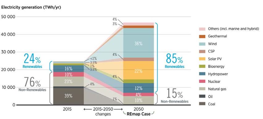
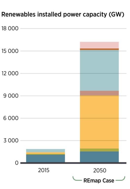
3

2 Background
This chapter provides the background knowledge and literature review relevant to this study. The first
section elaborates on the relevance, definition and implications of VRE. The second and third
subchapters address the challenges that occur with high shares of VRE in the power mix and the
approaches regarding VRE integration. 1 Section four, discusses power system planning. The fifth
section describes the difference between typical and atypical CF variability. Moreover, this subchapter
introduces and discusses the current variability inclusion approach, the TMY methodology.

2.1 Variable Renewable Energy
Shifting to higher shares of renewables in the power mix comes with several advantages, since
renewables mitigate climate change, reduce import dependency, and decrease the impact of fuel price
volatility. Moreover, due to the decreasing renewable power generation costs, renewables can
increasingly compete economically with fossil-based power plants.

In 2017 alone, 167 GW of renewable power generation capacity was added globally, of which solar PV
and wind accounted for 94 GW and 47GW, respectively. IRENA considers that a renewable-based
power sector is key to enable a sustainable energy future. The institute projects that in the best case
scenario, electricity consumption will double between 2015 and 2050 and that during the same time
span the share of renewables in the power mix will expand from 24% to 85% (see Fig. 1)[1].

This increase in renewables is mainly due to a strong growth in solar and wind power generation,
which together will make up 58% of generation in 2050. Solar PV and wind capacity are expected to
increase from 223 GW and 411 GW in 2015 to 7,122 and 5,445 GW in 2050 (see Fig. 2). Variable
renewable generation technologies, consisting mainly out of solar PV and wind, will make up 80% of
the annually added renewable power capacity [1].

 Fig. 1. Global Electricity Generation (TWh) Projection 2015-2050 [1].

1
 Throughout this document power refers to electric power

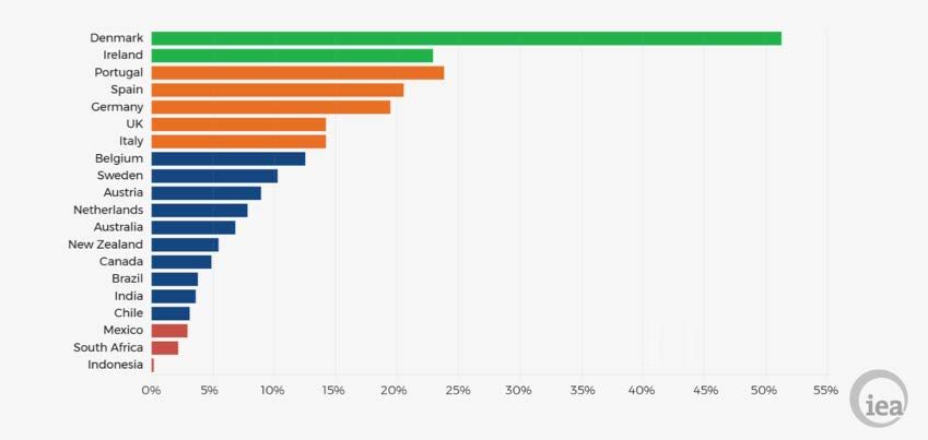
4

 Fig. 2. Global Installed Capacity (GW) Projection to 2015-2050 [1].

Amongst the renewables, VRE cannot be dispatched since the resources it relies on fluctuate and
cannot be stored. VRE technologies include wind power, wave and tidal power, run-of-river
hydropower and solar PV [4]. As illustrated by Fig. 3, several countries already operate power systems
with high shares of VRE e.g. Denmark with 51% and Portugal with 23% in 2016. This trend is expected
to continue [5]. Since the (free) fuels VRE relies on are inherently variable, VRE generation
technologies also pose a challenge.

 Fig. 3. Share of VRE in Power Mix (%)2016 [6].

2.1.1 VRE Generation Technologies: Wind and Solar PV
Most of variability in solar irradiation can be predicted, except for the part caused by the movement
of clouds [7]. Compared to solar, wind is less predictable, despite the presence of certain patterns.

5

Changes in solar PV output happen on a second-to-second base and are usually caused by clouds.
Hence, solar PV panels can face extreme variability during cloudy days. This variability tends to
decrease as solar PV panel are located increasingly scattered, geographically. Changes in wind output
occur throughout the temporal spectrum e.g. from second-to-second, to years [8]. NREL argues that
most wind variability happens in the scale of hours e.g. by an incoming storm front [7]. Moreover, the
institute found that the effect on output tends to be higher, compared to solar [7]. Like with solar,
geographic dispersion tends to reduce the aggregate variability of wind power. Regardless, wind
power availability can drop drastically in larger areas. Denmark and Germany, for instance, faced a 2
GW i.e. 90%, and 30 GW change in wind capacity, during the course of hours in 2007 and 2009,
respectively [8]. Hence, the availability of wind and solar radiance restricts production. The
consequent variable output i.e. variable CF, requires the power system to be able to adapt i.e. to be
flexible [2, 3].

2.2 VRE Challenges
As mentioned above, high VRE penetration levels can pose a challenge to power systems. According
to IRENA, the integrating high shares of VRE into existing grids is the key technical barrier for the
sustainable development of the power sector [9]. The following paragraphs will first address crucial
power system characteristics, by going into the power system stability, reliability and flexibility. The
following section elaborates on the difficulties that electricity market, grid operators, (conventional)
power plants, and the transmission and distribution system face when dealing with power systems
with high VRE shares.

2.2.1 Stable, Reliable and Flexible Power Systems
Basic power systems consist out of producers, consumers, their interconnection and system
operators. The latter is mandated with maintaining the balance between supply and demand and
ensure high power quality. This means that the end use can be performed without compromising
performance or equipment lifetime. To this goal, the power system needs to be reliable and stable.
The former refers to consumers receiving power when and how desired, whilst the latter addresses
the ability of the system to respond after facing a disturbance. Reliability is ensured via adequacy i.e.
managing to meet peak demand at all times, and security i.e. withstanding contingencies. Stability is
ensured via voltage, frequency and rotor angle stability [10].

Since VRE brings with it increasing variability and uncertainty of generation, power systems require
higher levels of flexibility. Flexible power systems can adapt to changes in supply and demand, besides
having the ability to manage dynamic conditions in general [11-13].

2.2.2 Challenges for Power System Actors
High shares of VRE can impact electricity markets, especially when the generation infrastructures are
relatively inflexible thermal heavy systems, by ‘distorting’ prices. As VRE plants can operate near to
zero variable costs, the marginal price of the power drops, thereby reducing wholesale prices. This
phenomenon is referred to as the ‘merit order effect’. On the other hand, prices may sharply increase
for short periods of time, where VRE resources are not available, as conventional power plants need
to ramp up [14].

Moreover, since actual VRE output might differ substantially from forecasted outputs, intraday prices
can deviate strongly from day-ahead prices. A sudden increase in VRE availability, combined with the
inability of thermal power plants to ramp down, can even drive prices below zero [14].

Third, variability in generation requires that operators have access to sufficient up and down ramps
to balance the system i.e. keep frequency and voltage within a stable range [7]. This network reserve

6

will likely be facilitated by fossil-fuel and hydroelectric generators. Consequently, these power plants
will need to alter their capacity level more frequently, including shutting down and turning on the
generators more often. This constitutes an increased physical strain on the installation, lowering
efficiency levels and increasing operational costs [7].

Next, as more demand is met with VRE-based electricity, the number of operating hours by
conventional power plant reduces, thereby decreasing the economic viability of the plant and hence
stalling new investments. This combined with low electricity prices makes it hard for conventional
power plants to cover costs [15].

Moreover, if VRE generation exceeds demand and the system lacks lower ramp capacity, VRE
generated power needs to be curtailed. This means that power which cannot be accepted by the grid
without destabilizing the system will be rejected. At these times, the VRE producer carries the
production costs, without renumeration [16].

Besides that, since VRE resources are often geographically scattered, they of lack connections to the
transmission and distribution system. Also, as single sites might have little installed capacity in place,
the grid needs to connect small-scale electricity generators using medium voltage and low voltage
networks. These are not as easy to manage in central dispatch stations, causing more reverse power
flows. This poses a physical strain on the transmission and distribution (T&D) system [4].

Besides the additional costs mentioned above, shortages or overloads might occur leading to brown-
and/or black-outs, if any of the system components or actors do not or cannot properly adjust to the
share of VRE in the system. Hence, VRE generation technology needs to be carefully integrated to
ensure the stability of the power system and to avoid unnecessary costs.

2.3 VRE Integration
As concluded in the previous section, VRE can challenge power system stability, reliability and
flexibility and can put a strain on several actors. However, the are several existing approaches to
facilitate the integration of high VRE shares. The following paragraphs will introduce these
approaches, followed by a smaller subsection dedicated to contingency planning.

Expanding as well improving the transmission and distribution network can strongly benefit the power
system in general and VRE integration in particular. First, by expanding the grid, one can make use of
the reduction in variability that tends to occur as the geographic coverage increases [4, 17-19].
Renewing existing T&D infrastructure, especially when dealing with relatively outdated hardware can
improve overall reliability and efficiency. This integration option requires relatively high level of
investment. Second, high shares of VRE often imply the democratization of production, leading to
many relatively small producers, i.e. prosumers, that both supply to and consume from the grid. This
can pose a strain on the grid, since most T&D infrastructure was not design for two-way traffic.
Addressing this technological bottleneck could directly contribute to getting more VRE from a larger
geographic area on the grid, thereby smoothing out variability [6, 20]. Moreover, grid codes should be
carefully be revised and synchronised to facilitate technology and electricity exchange amongst
different regions [6, 19].

Also, quickly dispatchable and flexible power plants, such as hydro and open gas turbines, secure the
power system. These generators can quickly adjust when sudden spikes or drops in VRE generation
occur, thereby avoiding imbalances in supply and demand as well as the consequent curtailments or
even black outs [4, 7, 19].

7

Besides that, empowering power system operators with certain tools increases their ability to manage
imbalances. First, real time generation and consumption data would allow system operators to
foresee and directly respond to imbalances. Second, access to curtailment options would enable the
operators to deal with unexpected overgeneration, in case the system does not have the required
down ramp capacities to handle sudden spikes in VRE generation [6].

Storage can enhance power system flexibility [4, 19]. There are several types of storage technologies,
including pumped hydro, thermal storage compressed air energy and batty storage, that could level
out generation variability [8].

Moreover, demand side management can improve power system performance. Demand patterns are
not stable, usually incorporating peak demand moments and sudden spikes in consumption.
Consequently, power producers need to adjust accordingly, by ramping up and turning on power
plants, or during low demand hours, by curtailing and storing power as well as ramping down and
turning off power plants. These actions tend to be costly and can pose somewhat of a risk. The latter
especially applies to high VRE penetrated system, in which production can suddenly spike or drop,
regardless of the load. Therefore, approaches such as peak-shaving, energy efficiency measures and
pricing incentives can help stabilize demand or align demand with supply [4, 17, 18, 21].

Additionally, market design can impact power system flexibility [7, 18]. First, larger markets tend to
be more flexible, and more cost-efficient in achieving and maintaining flexibility. This can be attributed
to the markets covering larger areas and including more capacity and consumers, thereby requiring
smaller proportions of reserves to safeguard reliability. This speaks in favour of extending access and
integrating power markets across borders. Here the Nordic Power Market poses an example, in which
Denmark sells wind when overproducing and can buy hydro power-based electricity from Norway and
Sweden if wind availability drops. Besides the size of power markets, the outlay can impact reliability,
stability and flexibility. Power market design varies strongly across the world; whilst some areas rely
on Power Purchasing Agreements (PPAs) set over long periods, other areas trade much closer to real
time via day-ahead and intra-day trading. In general, trading close to the time of delivery allows for
more efficient markets, especially if the installed capacity contains high VRE shares. Nevertheless, day-
ahead trading remains a vital component of current power systems, as they allow for the
consideration of physical limits, such as power plant ramping rates [4].

Additionally, VRE heavy power system systems can improve operations when having more insights
into when VRE generation will be available. This can be done by improving VRE forecasting. This
integration is perceived as relatively attractive, since it brings about little costs, whilst having a large
impact. Also, the required technologies are available commercially [7, 19, 22]. IEA argues that this, in
most cases, will not avoid black outs, but can reduce costs [6].

Last, by considering the impact of VRE on power system well in advance, i.e. during long-term planning
efforts, designs can be tailored to VRE characteristics. This requires that the tools that are being
deployed when planning power systems are adjusted accordingly [13, 17, 18, 23-25]. This study
focusses on this integration approach. More information on integrating VRE in long-term power
system planning is available in section 2.3, 2.4 and 2.5 of this report.

VRE integration bring about direct costs, e.g. ESMAP estimates the short-term integration costs of
wind to approximate 1-5 USD/MWh for systems that rely on less 10% on wind for generation, 3-5
USD/MWh for levels between 10 and 15% and 5-10 USD/MWh for to 15 to 30% wind generation [21].
These number pose and estimation and can differ strongly depending on the specific power system

8

design. Moreover, installing high shares of VRE generators combined with integration costs might be
more economic than installing conventional generators and thereby foregoing VRE integration costs.

The optimal integration strategy is country specific, however, elaborate planning can lower integration
costs in increase the seamless inclusion of high VRE shares [21].

2.3.1 Contingency Planning
Most system operators anticipate potential contingency event. Contingency planning ensures that e.g.
in the case of active power imbalance, system operators can tap into contingency reserves to maintain
frequency stability [13]. Thereby, the accuracy of contingency planning largely determines the
reliability of the power system [26]. Contingency planning is usually performed on a regional, if not
system level, for a period of multiple years [8]. This makes it a natural fit to long-term electricity
planning models. Yet, limited research has been dedicated to VRE specific contingency planning.

As a rule of thumb, the size of the contingency reserves equals the size of the largest contingency i.e.
the capacity needed to compensate for the loss of the equivalent of the largest generator or
transmission line [26].

2.4 Long-Term Power System Planning Models
Long-term electricity planning models used to assist capacity expansion and dispatch planning,
address time spans from 15 years or longer. Usually, these models have a top-down centralist
approach to identify potential future energy system design. This data again is used to assist policy
makers with decision making and to identify investment options [13].

Long-term power system planning models are instrumental in facilitating VRE integration [13, 19].
However, with the share of renewable energy in the power sector increasing from 25% in 2017 to 85%
in 2050, new approaches to power system planning will be required [1]. The next two subchapters
address the VRE attributes that need to be considered in long-term power system planning and the
specific modelling approach used in this study, least-cost power system planning.

2.4.1 High VRE Shares in Power System Planning
VRE has several characteristics that require consideration when performing capacity extension
simulations. These can roughly be divided in five larger attributes.

The first attribute is variability. With higher VRE shares the net load becomes increasingly variable.
This is due to the variability in CF over time and space. This is relevant for power system planning
tools, since these will require distinct spatial and temporal granularity to capture VRE and load
interaction [23]. Also, since VRE availability varies geographically, it is of importance that the
transmission and distribution network is included in the analysis, with a relatively high level of detail
[23].

A second relevant attribute is uncertainty. Since weather cannot be perfectly forecasted, the amount
of electricity generated by VRE at a certain point of time has a relevant uncertainty level. This bring
up a need for models to take this into account, by installing appropriate amounts of operating
reserves, which flexible enough ramping rates [23].

Third, the near zero marginal cost mentioned above (or even negative cost when near zero cost are
complemented with subsidies), mean that VRE related economic indicators e.g. high fixed costs,
capacity-based subsidies, and their consequent influence on market operations and behaviour must
be included [23].

9

Fourth, due to relatively low yet varying CF values, generation might or might not coincide with
demand, which can compromise resource adequacy and system reliability [23].

Fifth, in the case of excess generation and limited down ramping options, VRE-based electricity might
face curtailment. This phenomenon needs to be included in power planning tools, using load and VRE
data with a temporal component, as well as data on conventional generators e.g. minimum generation
[23].

Hence, as the power system is undergoing a VRE-heavy transformation, long-term power system
planning models need to follow suit to facilitate effective power system planning and VRE integration.
Power system planning tools come in many shapes and sizes, the next section of this document will
elaborate of the sort of capacity expansion and dispatch model used in this study.

2.4.2 Least Costs Power System Planning Models
This study uses a capacity expansion and dispatch model type, labelled least costs power system
planning model. Least costs power system planning is a commonly used methodology to determine
optimal capacity expansion and dispatch strategies. This type of model determines what generators
should be added to the system and when what generators should run at what capacity to minimize
costs [27-31]. The methodology numerically minimizes or maximizes the value of the key equation i.e.
objective function, under certain constraints, using linear programming (LP). Hence, in least cost
power system planning the objective function is the cost equation, which is subjected to constraints
(e.g. maximum spending) or contains variables and parameters that are limited by constraint (e.g.
emission caps or spinning reserve requirements).

The model requires input data on e.g. the capital expenditures (CAPEX), operational expenditures
(OPEX) or the ramping rate of generators as well as data on demand and in the case of VRE such as
wind or solar, detailed available capacity data [27, 32]. The latter, usually referred to as the CF is key,
since it reflects the variability that the generator faces and thereby the power it can provide at a
certain time. As the share of renewables in the power system increases, the importance of CF data
reliability strongly increases [24]. However, due to computational restrictions, the CF data usually is
compressed by reducing the resolution [33]. There are several approaches to do so, of which the
typical meteorological year (TMY) approach is widely spread [34-39].

2.5 Atypical vs. Typical Variability
While solar and wind variability is well known, the computational complexity of dealing with power
system planning models means multi-year details have to be compressed [33]. There are several
approaches to do so, of which the typical meteorological year (TMY) approach is most common [34-
39]. The TMY originally is a conglomerate of weather data with, typically with an hourly resolution,
that describes a typical annual weather pattern e.g. temperature, air humidity, wind speeds and
direction, and radiation [35]. When applied to power system planning, the output can be given as
wind speed or solar radiance, or alternatively as CF. In this study, the latter applies. There are several
different approaches to collating TMY, ranging from the Danish method, the ISO-defined TMY
approach, Weather Year for Energy Calculation (WYEC) to the most recent modification of the
American used TMY, TMY3 [35, 40].

However, as the TMY purposely aims at being ‘typical’, deviations are often excluded and due to the
resolution reduction, atypical CF variability is smoothened out [35]. Atypicality can e.g. be visualized
as a sunny day in winter harvesting more solar power than a cloudy day in summer. This is a case of
atypical intra-annual variability. A second example is a year with unusually low or high wind

10

availability, which represents a case of a typical inter-annual variability [25]. A dataset including typical
and atypical inter- and intra- variability would pose a more realistic description of VRE availability.

Previous studies have found that reducing temporal resolution to capture solar data distorts power
system planning outcomes. References [41] and [42] find that low temporal resolution leads to the
overestimation of the VRE uptake. Moreover, low temporal resolution causes the overestimation of
VRE and flexible base load technologies investment, paired with the underestimation of the optimal
investment in flexible dispatchable generation technologies [41, 42]. Reference [24] also finds that
oversimplifying VRE dynamics leads to the overestimation of VRE generation, which in their case
amounts up to 9% of electricity demand [24]. Reference [43] finds that demand-supply mismatch is
not fully represented. They expand the MESSAGE model by adding trade-offs between VRE
deployment and consequent integration costs e.g., via system flexibility, electricity curtailment and
backup capacity. This is instrumental in representing the shadow costs of VRE integration. However,
they do not address the CF reduction issue [43]. Reference [44] finds that the representative days
approach to compressing data is better suited for high VRE system, than the integrated approach and
establishes that a minimum of 160 time steps is required to avoid systematically overestimating
renewable capacity shares. Reference [25] demonstrates that there is high inter-annual variability in
solar PV and wind power output in the United Kingdom, when analysing a 25-year time-series data
set, including that sunny days in winter, might harvest more than cloudy days in summer, a
phenomenon which is not represented in lower resolution input data. Moreover, [25] finds that
models with high VRE shares using few input years are unreliable. Hence, there is a clear need for long
time series to reflect variability in order to perform proper power system planning. The United
Kingdom case study concludes that individual years harvest significantly different power system than
TMY and suggests avoiding the usage of TMY [25]. Also, [45] as well as [35] found that TMY based
power system plans significantly differ from plans using actual time-series CF input data [35, 45].
Several other studies also find that different TMY methods harvest significantly different power
system designs [40, 46-48].

Previous studies exclusively focus on how TMY effects power system design. This study differentiates
itself by analysing the consequences of deploying TMY-based power systems, i.e., by assessing TMY-
based power system performance when exposed to atypical conditions. Besides that, this study is the
first of its kind to quantify the effect of the TMY approach in foregone generation, additional costs,
unmet demand and additional CO2 emissions.

Moreover, this study explores additional side tracks, that have not been explored before. First is the
effect of reserve and solar contingency planning on power system performance and design, also
addressing batteries as stability measure. Second, this study proposes a novel data reduction
methodology, constituting out of adding years incrementally in a simplified capacity expansion model,
to determine the required number of input years to achieve the optimal solution. Additionally, the
performance analyses mentioned before can in itself be used, to identify during what years the system
over- or underperforms. Thereby, this approach is a novel data reduction methodology. Also, the
performance analysis allows solutions to be tailored to specific years, rather than for the entire time
series.

Besides that, this study covers case studies that have not been explored before, Turkey and Guinea-
Bissau. The Guinea-Bissau case study explores an increasing common scenario, in which relatively
small power system heavily rely solar PV, that has not been studied before.

11

3 Country Profile: Guinea-Bissau
Guinea-Bissau is located on the west coast of the African continent, between Senegal and Guinea,
bordering the North Atlantic Ocean. The country covers a surface of 38,125 km2, and has a population
of 1.79 million [49].

3.1 Socio-Economic Profile
Approximately 40% of the population lives in urban areas, and 20% of the population lives in the
capital city of Bissau. 60% of the population is younger than 25 years of age. The fertility rate is over
4 children per women. At the same time the country faces high infant and maternal mortality rates.
The country has been subjected to political instability with the last coup taking place in 2012 [49]. In
2015, Guinea-Bissau ranked 178st out of 188 countries in the Human Development Index, with a value
of 0.424 [50].

In 2017, the country had 3 billion USD worth of GDP, i.e. 1,800 USD GDP per capita. GDP growth rate
approximated 5% in the same year. In 2015, 67% of the population lived below the poverty line.
Agriculture, services and industry each composed 44%, 43%, 13% of GDP. In 2000, 82% of the labour
force was employed by the agricultural sector, and the remaining 18% by industry and services [49].

3.2 Energy System and Resources
In 2015, Guinea-Bissau consumed 26,829 TJ of energy, of which biofuels made up the vast majority
(see Fig. 4). All biomass-based energy was consumed by the residential sector, and mainly consists out
of fuelwood that is burned directly, or used for charcoal production [51]. The second largest
contributor, oil, stemmed from imports and was consumed by road transport. Charcoal, produced
from biomass, amounted for 8% of consumption. The remaining 1% of electricity was generated using
imported oil and is mainly consumed in the manufacturing and residential sector [52].

 8% 1% 12%

 79%

 Oil Primary biofuels and waste Charcoal Electricity

 Fig. 4. Energy Consumption by Source (%)Guinea-Bissau 2015 [52].

Despite favourable conditions little renewable resources are being harvested [53]. Domestically,
Guinea-Bissau has vast solar resources with 3,000 hours of sun per year with an average solar radiation
of 4.5 to 5.5 kWh/m2/day [53, 54]. Moreover, the Geba river and the Rio Corubal have a combined
estimated hydroelectric capacity of 184 MW. Until date this resource is not being tapped for electricity
generation. Also, due to the coastline, tidal energy could be viably harvested. A 500 MW tidal plant
was announced in 2015. Along the coast wind speed is estimated around 2.5 to 7 m/s. There are no
plans to date to utilize this potential. No geothermal surveys have been conducted to date. Moreover,

12

no economically viable oil or natural gas reserve where proven to date in Guinea-Bissau [54]. In 2015,
Guinea-Bissau imported 5,171 TJ oil and exported 3 TJ worth of charcoal [52].

3.3 Electricity System
The electrification rate increased compared to the 0% in 1990 but remains low at 15% in 2016. The
majority of people with access are located in urban areas, where availability is limited to 70% of the
time [55].

In 2015, 36 GWh of electricity was produced in Guinea-Bissau. All electricity was generated by 28 MW
thermal capacity with approximately 33% efficiency. The residential sector consumed 15 GWh of this
electricity, the remaining 21 GWh was consumed by the industrial sector [56].

The electricity system has 72 MW of committed capacity that will be installed by 2019, running on
heavy fuel oil (HFO) [57]. The Government of Guinea-Bissau intends to expand its power system, as
peak demand is projected to increase to 155 MW by 2030, thus by far exceeding the committed 72
MW. Currently, the costs of generation are relatively high with 135 USD/MWh. This is due to the high
dependency on HFO, which is a relatively expensive fuel. However, the costs might come down to 100
USD/MWh if LNG were to become available [57].

3.4 Energy Policy
In Guinea-Bissau the Ministry of Energy and Industry is responsible for the energy sector, whilst the
National Electricity and Water Corporation (EAGB) is in charge of the electricity sector. The national
energy policy landscape stems mainly from the 2013 Energy Master Plan and the Intended Nationally
Determined Contributions (INDCs) [51].

During the Paris climate agreement in 2015, the Government of Guinea-Bissau, formulated 3 main
energy-related INDCs. First, renewables should make up 80% of the national energy mix by 2030.
Second, energy losses are to be reduced down to 10% until 2030, by increasing energy efficiency.
Third, the country aims to reach 80% of universal electricity access by 2030.

Moreover, a national action plan for renewable energy in Guinea-Bissau was published in 2017, along
the lines of the SE4ALL framework [58, 59]. The latter states that the country aims for 72 MW of
installed renewable capacity by 2030, that should cover 52% of demand. Of this 72 MW, 15 MW, i.e.
11% is due to be solar. Wind accounts for 2 MW, i.e. approximately 1%.

Also, Guinea-Bissau is a member of the West African Power Pool (WAPP), a regional initiative to
integrate national power operators into an unified electricity market, harmonize electricity planning
and increase transboundary reliable electricity exchanges [51, 60].

3.5 Solar PV CF Variability
The Guinea-Bissauan solar PV CF variability illustrated in this section, bases on a timeseries describing
solar PV output, covering 24 years, ranging from 1994 to 2017 [61]. As illustrated by Fig. 5, the annual
average solar PV CF in Guinea-Bissau has been stable over the last 24 years, with an average of 18.3%
and a low standard deviation of approximately 0.3%. Also, the average hourly CF throughout the years
amounts to the typical bell-shaped curve, peaking at approximately 60% around noon, as illustrated
by Fig. 6. However, these average values do not imply the absence of variability. Fig. 6 also shows the
coefficient of variation for each individual hour. Even during the more stable hours, i.e. from 12AM to
3PM the standard deviation is approximately 25% of the mean. In the early morning and late evening
hours this number increases to 100% and 200% respectively, illustrating the even higher solar PV CF
variability present around sunset and sunrise. The high average variability around sunset and -rise can
be largely attributed to the seasonal variation.