Analysis of the water-power nexus in the North, Eastern and Central African Power Pools

Analysis of the water-power nexus in the
North, Eastern and Central African Power
Pools

 Authors:
 PAVIČEVIĆ, M., QUOILIN, S.,

 Editors:
 DE FELICE, M.,
 BUSCH, S.,
 HIDALGO GONZÁLEZ, I.

 2020

 EUR 30310 EN

This publication is a report prepared by the Katholieke Universiteit Leuven for the Joint Research Centre (JRC), the European
Commission’s science and knowledge service. It aims to provide evidence-based scientific support to the European policymaking process.
The scientific output expressed does not imply a policy position of the European Commission. Neither the European Commission nor any
person acting on behalf of the Commission is responsible for the use that might be made of this publication. For information on the
methodology and quality underlying the data used in this publication for which the source is neither Eurostat nor other Commission
services, users should contact the referenced source. The designations employed and the presentation of material on the maps do not
imply the expression of any opinion whatsoever on the part of the European Union concerning the legal status of any country, territory,
city or area or of its authorities, or concerning the delimitation of its frontiers or boundaries.

Contact information
Name: Ignacio Hidalgo González
Address: European Commission, Joint Research Centre (JRC), P.O. Box 2, NL-1755 ZG Petten, The Netherlands
Email: Ignacio.HIDALGO-GONZALEZ@ec.europa.eu
Tel.: +31224565103

EU Science Hub
https://ec.europa.eu/jrc

JRC121098
EUR 30310 EN

 PDF ISBN 978-92-76-20874-7 ISSN 1831-9424 doi:10.2760/12651

Luxembourg: Publications Office of the European Union, 2020

© European Union, 2020

The reuse policy of the European Commission is implemented by the Commission Decision 2011/833/EU of 12 December 2011 on the
reuse of Commission documents (OJ L 330, 14.12.2011, p. 39). Except otherwise noted, the reuse of this document is authorised under
the Creative Commons Attribution 4.0 International (CC BY 4.0) licence (https://creativecommons.org/licenses/by/4.0/). This means that
reuse is allowed provided appropriate credit is given and any changes are indicated. For any use or reproduction of photos or other
material that is not owned by the EU, permission must be sought directly from the copyright holders.

All content © European Union 2020

How to cite this report: Pavičević, M. and Quoilin, S., Analysis of the water-power nexus in the North, Eastern and Central African Power
Pools, De Felice, M., Busch, S. and Hidalgo Gonzalez, I., editor(s), EUR 30310 EN, Publications Office of the European Union,
Luxembourg, 2020, ISBN 978-92-76-20874-7, doi:10.2760/12651, JRC121098.

Contents

Foreword .....................................................................................................................................................................................................................................................................1
Acknowledgements...........................................................................................................................................................................................................................................2
Abstract........................................................................................................................................................................................................................................................................3
1 Introduction .....................................................................................................................................................................................................................................................4
 1.1 Overview of the African power pools .......................................................................................................................................................................4
 1.2 Policy context...................................................................................................................................................................................................................................5
 1.3 Data uncertainty ...........................................................................................................................................................................................................................6
 1.4 Structure of the report ...........................................................................................................................................................................................................6
2 Modelling framework .............................................................................................................................................................................................................................7
 2.1 Models used within this study .........................................................................................................................................................................................7
 2.1.1 LISFLOOD ..........................................................................................................................................................................................................................7
 2.1.2 TEMBA – OSeMOSYS ..............................................................................................................................................................................................8
 2.1.3 Dispa-SET ..........................................................................................................................................................................................................................8
 2.2 Methods and assumptions ..................................................................................................................................................................................................9
 2.2.1 Hydro inflows and availability factors ..................................................................................................................................................9
 2.2.2 Wind and solar availability factors ....................................................................................................................................................... 10
 2.2.3 Fuel prices .................................................................................................................................................................................................................... 10
 2.3 Power system metrics and indicators .................................................................................................................................................................. 11
 2.3.1 RES curtailment ....................................................................................................................................................................................................... 11
 2.3.2 Shed load and lost load .................................................................................................................................................................................. 11
 2.3.3 Shadow price ............................................................................................................................................................................................................. 11
 2.3.4 Water stress ............................................................................................................................................................................................................... 11
 2.3.5 Water exploitation index ................................................................................................................................................................................. 12
 2.3.6 Water value ................................................................................................................................................................................................................. 12
 2.3.7 Start-ups ........................................................................................................................................................................................................................ 12
 2.3.8 CO2 emissions ........................................................................................................................................................................................................... 12
3 Input data and assumptions ....................................................................................................................................................................................................... 13
 3.1 African power pools ............................................................................................................................................................................................................... 13
 3.2 Fuel prices....................................................................................................................................................................................................................................... 13
 3.2.1 Local resource availability (biomass/biogas, peat and coal) ....................................................................................... 14
 3.3 Hourly load profiles ............................................................................................................................................................................................................... 14
 3.4 Supply ................................................................................................................................................................................................................................................. 15
 3.5 Hydropower units ..................................................................................................................................................................................................................... 17
 3.5.1 Evapotranspiration ............................................................................................................................................................................................... 19
 3.5.2 Inflows ............................................................................................................................................................................................................................. 19
 3.6 Thermal units............................................................................................................................................................................................................................... 20

 i

3.7 Grid infrastructure .................................................................................................................................................................................................................. 20
4 Scenarios ....................................................................................................................................................................................................................................................... 23
 4.1 Reference scenario ................................................................................................................................................................................................................. 23
 4.2 Connected scenario................................................................................................................................................................................................................ 24
5 Results and discussion of the Reference and Connected scenarios .................................................................................................... 25
 5.1 Storage levels computed by Dispa-SET MTS ................................................................................................................................................ 25
 5.2 Total system costs ................................................................................................................................................................................................................. 27
 5.3 Shadow prices ............................................................................................................................................................................................................................. 27
 5.3.1 Reference scenario .............................................................................................................................................................................................. 27
 5.3.2 Connected scenario ............................................................................................................................................................................................. 28
 5.4 Electricity generation ........................................................................................................................................................................................................... 29
 5.4.1 Reference scenario .............................................................................................................................................................................................. 31
 5.4.2 Connected scenario ............................................................................................................................................................................................. 31
 5.5 Curtailment and spillage .................................................................................................................................................................................................. 31
 5.6 Load shedding ............................................................................................................................................................................................................................ 32
 5.6.1 Reference scenario .............................................................................................................................................................................................. 32
 5.6.2 Connected scenario ............................................................................................................................................................................................. 34
 5.7 Start-ups .......................................................................................................................................................................................................................................... 34
 5.8 Water stress and water value ..................................................................................................................................................................................... 37
 5.8.1 Reference scenario .............................................................................................................................................................................................. 37
 5.8.2 Connected scenario ............................................................................................................................................................................................. 40
 5.9 Water values ................................................................................................................................................................................................................................ 41
 5.10 CO2 emissions ............................................................................................................................................................................................................................. 42
6 Long-term simulations: soft linking with TEMBA .................................................................................................................................................... 44
 6.1 PV, Wind and CSP .................................................................................................................................................................................................................... 44
 6.2 TEMBA Scenarios...................................................................................................................................................................................................................... 44
 6.3 Power supply ................................................................................................................................................................................................................................ 45
 6.3.1 NTC ...................................................................................................................................................................................................................................... 46
 6.4 Results and discussion from TEMBA scenarios........................................................................................................................................... 47
 6.4.1 Generation .................................................................................................................................................................................................................... 47
 6.4.2 Curtailment .................................................................................................................................................................................................................. 48
 6.4.3 Load shedding .......................................................................................................................................................................................................... 48
 6.4.4 Fresh water withdrawal and consumption.................................................................................................................................... 49
 6.4.5 CO2 emissions ........................................................................................................................................................................................................... 50
 6.4.6 Adequacy of the TEMBA system ............................................................................................................................................................. 51
7 Conclusions ................................................................................................................................................................................................................................................. 52
8 References ................................................................................................................................................................................................................................................... 53
List of abbreviations and definitions........................................................................................................................................................................................... 55
List of figures..................................................................................................................................................................................................................................................... 56

 ii

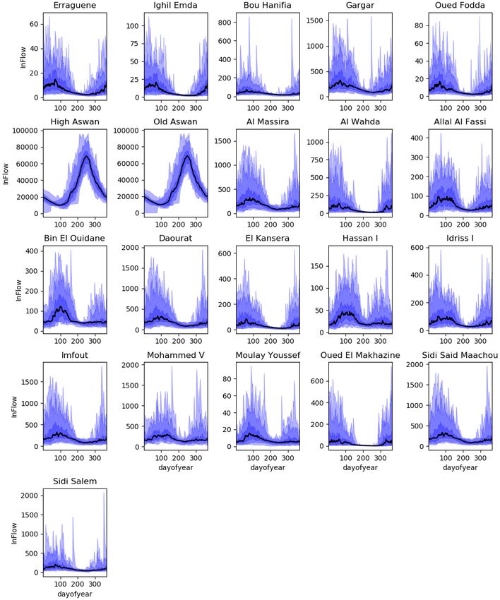
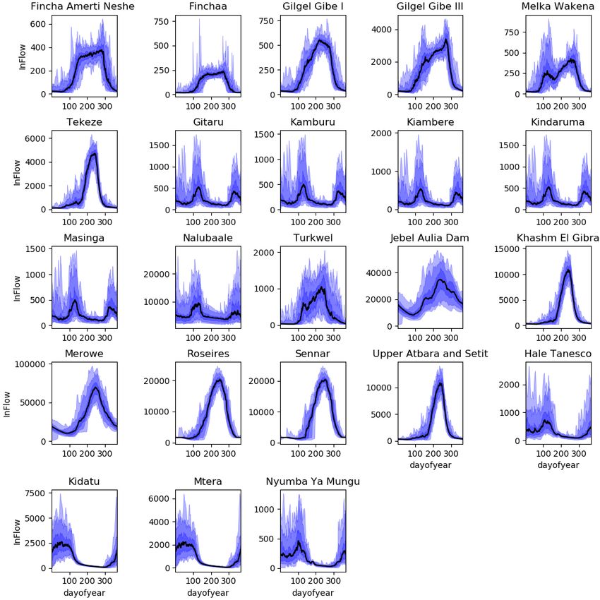
List of tables ....................................................................................................................................................................................................................................................... 59
Annexes.................................................................................................................................................................................................................................................................... 60
 Annex 1. Fuel price estimation ................................................................................................................................................................................................. 60
 Annex 2. Hydro units statistics ................................................................................................................................................................................................. 64
 Annex 3. Typical units ....................................................................................................................................................................................................................... 65
 Annex 4. Renewable capacity factors ................................................................................................................................................................................ 66
 Annex 5. Historical inflows ........................................................................................................................................................................................................... 68
 Annex 6. Shadow prices .................................................................................................................................................................................................................. 71
 Annex 7. Generation ........................................................................................................................................................................................................................... 75
 Annex 8. Curtailment ......................................................................................................................................................................................................................... 78
 Annex 9. Load shedding .................................................................................................................................................................................................................. 80
 Annex 10. Water indicators ......................................................................................................................................................................................................... 83
 Annex 11. CO2 emissions ............................................................................................................................................................................................................... 89

 iii

Foreword
Increasing water stress will intensify competition between water uses. A lack or an excess of water may
undermine the functioning of the energy and food production sectors with societal and economic effects.
Energy and water are inextricably linked: we need “water for energy” for cooling thermal power plants, energy
storage, biofuels production, hydropower, enhanced oil recovery, etc., and we need “energy for water” to pump,
treat and desalinate. Without energy and water, we cannot satisfy basic human needs, produce food for a
rapidly growing population and achieve economic growth. Producing more crops per drop to meet present and
future food demands means developing new water governance approaches.
The Water Energy Food and Ecosystem Nexus (WEFE Nexus) flagship project addresses in an integrated way
the interdependencies and interactions between water, energy, agriculture, as well as household demand. These
interactions have been so far largely underappreciated. The WEFE-Nexus can be depicted as a way to overcome
stakeholders’ view of resources as individual assets by developing an understanding of the broader system. It
is the realization that acting from the perspective of individual sectors cannot help tackle future societal
challenges.
The overall objective of the Water-Energy-Food-Ecosystems Nexus flagship project (WEFE-Nexus) is to help in
a systemic way the design and implementation of European policies with water dependency. By combining
expertise and data from across the JRC it will inform cross-sectoral policy making on how to improve the
resilience of water-using sectors such as energy, agriculture and ecosystems.
WEFE-NEXUS objectives
— Analyse the most significant interdependencies by testing strategies, policy options and technological
 solutions under different socio-economic scenarios for Europe and beyond.
— Evaluate the impacts of changing availability of water due to climate change, land use, urbanization,
 demography in Europe and geographical areas of strategic interest for the EU.
— Deliver country and regional scale reports, outlooks on anomalies in water availability, a toolbox for
 scenario-based decision making, and science-policy briefs connecting the project’s recommendations to
 the policy process.
How is the analysis done?
JRC experts use a broad range of models and sources to ensure a robust analysis. This includes water resources
and climate models to understand current and future availability of water resources, and energy models and
scenario employed to understand and forecast current and future energy demands and the related water
footprint of the energy sector.
The results from these models are expected to provide i) understanding the impacts of water resources on the
operation of the energy system, and vice versa, ii) spatial analysis and projection of water and energy
requirements of agricultural and urban areas in different regions, iii) producing insights for a better
management of water and energy resources.
What is this report about?
The WEFE projects aims to provide a detailed insight of the water-power nexus in all African power pools, since
the power system is the most water-intensive part of the energy industry. This report provides the results of
the model-based analyses carried out for the North (NAPP), Central (CAPP) and Eastern (EAPP) African Power
Pool according to the approach used by the JRC for the West African Power Pool (De Felice et al., 2018), and
the Iberian Peninsula (Fernandez Blanco Carramolino et al., 2017).

 1

Acknowledgements
This report has been prepared by the Mechanical Engineering Technology unit of The Katholieke Universiteit
Leuven (KUL) for the European Commission's Joint Research Centre, under service contract 938088, therefore
the content of this study does not reflect the official opinion of the European Union. Responsibility for the
information and views expressed in the study lies entirely with the authors.
We thank you the comments and suggestions from our colleagues Andreas Uihlein and Stathis Peteves.

Authors (KUL)
Matija Pavičević
Sylvain Quoilin

Editors (JRC)
Sebastian Busch
Matteo De Felice
Ignacio Hidalgo González

 2

Abstract
This report describes the results of applying an open-source modelling framework to three African power pools1:
the Central African Power Pool, the Eastern Africa Power Pool and the North African Power Pool. The modelling
framework is used to analyse results at country level - where insights regarding the power generation, system
adequacy, total operational costs, freshwater consumption and withdrawals, water values (hydro storage
shadow price), and CO2 emissions linked to the power sector are assessed. The model source code and the
input data are provided together with the report for transparency purposes to facilitate further exploitation and
analysis of the results.
Water-energy nexus indicators such as the water exploitation index, or water withdrawal and consumption
related to power generation, are computed for the three power pools and for major individual power plants.
The indicators show that these three African Power Pools are strongly dependent on the availability of
freshwater resources. The variation between wet and dry years significantly impacts the final energy mix, the
total operational costs, the total carbon emissions and the water stress index of the system. The relative impact
of water consumption2 over water withdrawals3 is low because of the predominance of once-through cooling
systems in the most vulnerable countries.
Furthermore, several isolated countries within each power pool exhibit a power system which is not adequate,
leading to significant amounts of load not served. The importance of increasing the reliability as well as the
capacity of interconnection lines is thereby highlighted. A well interconnected grid reduces the need for variable
renewable energy (VRES) curtailment and water spillage in hydropower units, allows higher integration of
renewable sources, and reduces the need for load shedding4, especially in extremely dry years. A higher degree
of interconnection also has a positive impact on water stress indicators since water consumption and water
withdrawal can be significantly reduced.
Africa presents an important potential of variable renewable energy sources (mainly wind and solar) which is
still largely untapped. The addition of new VRES capacity can reduce the potential carbon emissions by more
than 32% by 2045 compared to a business-as-usual scenario. However, this is only possible by reducing the
congestion when energy flows from southern countries (hydro-rich), and energy flows from the northern
countries (VRES-abundant) are enabled. This is particularly the case in future low carbon scenarios, in which
power generation from thermal units is lower, resulting in a lack of flexibility and therefore in higher curtailment
and load shedding.

1
 Regional cooperation entities aimed to developing a common power grid and a common market between their members.
2
 Water lost due to evaporation, leakages, or rendered unusable through other thermo-chemical processes.
3
 Thermal pollution due to the increased water temperature caused by cooling processes inside the power plants.
4
 An additional safety mechanism that can be enforced to prevent system blackouts, usually provided by large industrial facilities which
 can decrease their production for a certain amount of time.

 3

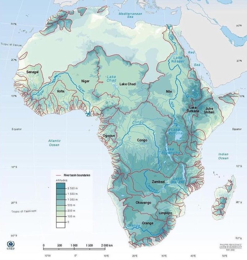
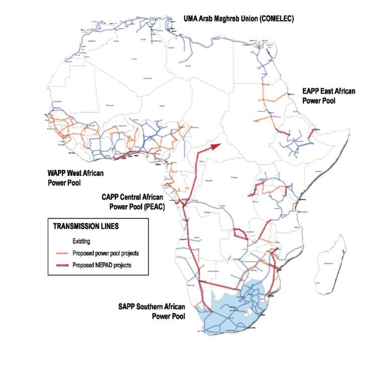
1 Introduction
Access to a stable and secure supply of energy is a fundamental driver of economic growth in Africa. More
than two-thirds of the population, approximately 600 million people, especially in Sub-Saharan Africa, lacked
access to electricity in 2016, and 850 million people had no access to clean cooking facilities such as natural
gas, liquefied petroleum gas, electricity and biogas, or improved biomass cook stoves (International Energy
Agency, 2017). Africa’s gross economic activity is, according to (African Development Bank Group, 2019),
expected to continue its rapid growth. The economic growth is estimated at 4.1% in 2019 compared to 2.4%
in 2018 and is set to increase between 2.1 and 4.1% annually in the next decade5. In order to meet this growing
demand, and take advantage of trade opportunities, five regional power pools (regional cooperation entities
aimed to developing a common power grid and a common market between their members) have been
established.

1.1 Overview of the African power pools
The geographical overview of the power pools studied in this report is presented in Figure 1, while their
statistical data are shown in Table 1. This study complements similar analyses carried out directly by the JRC
and therefore focuses only on three power pools, namely:
— the Central African Power Pool (CAPP) 6 Angola, Cameroon, Central African Republic, Chad, Congo,
 Democratic Republic of Congo (DRC), Equatorial Guinea and Gabon;
— the East African Power Pool (EAPP) 7, DRC, Djibouti, Egypt, Ethiopia, Kenya, Rwanda, Somalia, Sudan,
 Tanzania, Libya, Uganda and South Sudan; and
— the North African Power Pool (NAPP) 8 Algeria, Libya, Mauritania, Morocco and Tunisia.

 Figure 1 Organization of African power pools

 Source: (Medinilla, Byieres, and Karaki, 2019)

5
 The World Bank: https://data.worldbank.org/indicator/NY.GDP.MKTP.KD.ZG?locations=ZG
6
 CAPP Geographic Information System: https://www.peac-sig.org/en/
7
 East African Power Pool: http://eappool.org/
8
 Comité Maghrébin de l'Electricité (COMELEC): https://comelec-net.org/index-en.php

 4

Table 1 Statistics for the three power pools.

 Electricity
 Country names GDP per capita Electricity use
 Population 2018 consumption per
 Power and 2018 (change rate 2017 (total,
 (change from capita 2015
 Pool corresponding from 2010), urban and rural)
 2010), millions (change from
 ISO-2 code USD %
 2010), kWh
 Angola (AO) 30.8 (+7.4) 3 432 (-155) 312 (+105) 41.8 / 72.7 / 0.0
 Cameroon (CM) 25.2 (+4.9) 1 533 (+248) 275 (+14) 61.4 / 93.2 / 21.3
 Central African
 4.7 (+0.3) 475 (-12) 29.9 / 52.1 / 14.6
 Republic (CF)
 Chad (TD) 15.5 (+3.5) 728 (-163) 10.8 / 39.1 / 2.4
 Congo (CG) 5.2 (+1.0) 2 147 (-661) 203 (+63) 66.2 / 87.4 / 24.2
 CAPP
 Democratic
 Republic of the 84.0 (+19.5) 561 (+228) 108 (+4) 19.1 / 49.2 / 0.0)
 Congo (CD)
 Equatorial
 1.3 (+0.4) 10 261 (-7,001) 67.1 / 91.3 / 6.0
 Guinea (QE)
 Gabon (GA) 2.1 (+0.5) 7 952 (-888) 1 168 (+210) 92.2 / 97.5 / 49.1
 Burundi (BI) 11.2 (+2.5) 272 (+38) 9.3 / 61.8 / 1.7
 Djibouti (DJ) 1.0 (+0.1) 3 083 (+1,740)
 Egypt (EG) 98.4 (+15.7) 2 549 (-96) 1 683 (+107) 100 / 100 / 100
 Eritrea (ER) 3.2 (+0.0) 332 (-336)
 Ethiopia (ET) 109.2 (+21.6) 772 (+431) 69 (+21) 44.3 / 96.6 / 31
 Kenya (KE) 51.4 (+9.4) 1 711 (+759) 164 (+16) 63.8 / 81.1 / 57.6
 EAPP Rwanda (RW) 12.3 (+2.3) 773 (+190) 34.1 / 84.8 / 23.6
 Somalia (SO) 15.0 (+3.0) 315 (+47)
 South Sudan
 11.0 (+1.5) 353 (-1,182)
 (SS)
 Sudan (SD) 41.8 (+7.3) 977 (-513) 190 (+59) 56.5 / 82.5 / 42.8
 Tanzania (TZ) 56.3 (+12.0) 1 050 (+307)
 Uganda (UG) 42.7 (+10.3) 643 (+20)
 Algeria (DZ) 42.2 (+6.3) 4,115 (-366) 1 363 (+346) 100 / 100 / 100
 Libya (LY)* 6.7 (+0.5) 7 242 (-4,823) 1 811 (-1,551) 70.1 / 70.1 / 70.1
 NAPP Mauritania (MR) 4.4 (+0.9) 1 189 (-53) 42.9 / 82.6 / 0
 Morocco (MA) 36.0 (+3.7) 3 238 (+398) 904 (+128) 100 / 100 / 100
 Tunisia (TN) 11.6 (+0.9) 3,448 (-694) 1 455 (+90) 100 / 100 / 100
Source: The World Bank Data

The renewable and fossil potentials vary significantly between the power pools. NAPP is mostly dominated by
fossil while CAPP and EAPP are dominated by water. Most diverse, by per country basis is EAPP where some
countries are either entirely fossil or almost entirely renewable powered.

1.2 Policy context
The European Commission’s Comprehensive Strategy with Africa (European Commission, 2020), the United
Nation's Sustainable Energy for All 9 and the Power Africa10 initiatives aim to electrify some 60 million homes
and support the investment of 30 GW of clean power generation in the near future. Despite this, however, there
is no coherent ‘by country’ and ‘by region’ set of concrete scenarios besides the ones proposed in (Taliotis et
al., 2016; Pappis et al., 2019), nor an open energy system analysis platform that may be used to carry out a
more detailed investigation of the proposed long term power generation expansion scenarios. However, there
are several studies based on non-open modelling frameworks such as JRC’s GECO (Keramidas et al., 2020) and
IEA’s WEO (IEA, 2020) among others.

9
 Sustainable Energy for All (SEforALL) - an international organization working with leaders in government, the private sector and civil
 society to drive further, faster action toward achievement of Sustainable Development Goal 7 (SDG7), which calls for universal access
 to sustainable energy by 2030, and the Paris Agreement, which calls for reducing greenhouse gas emissions to limit climate warming
 to below 2° Celsius. https://www.seforall.org/about-us
10
 Power Africa - project development in sub-Saharan Africa’s energy sector. www.usaid.gov/powerafrica

 5

The term “water-energy nexus” refers to the complex interactions between water resources (especially
freshwater) and the energy sector. The combined effect of increased water consumption, for energy and non-
energy purposes, with lower availability of water resources due to climate change is expected to lead to
monetary losses, power curtailments, temporary shutdowns and demand restrictions in power grids across the
world (Fernandez Blanco Carramolino et al., 2017). These consequences highlight the need for an integrated
modelling framework for the water and power sectors capable of analysing such cross-sectoral interactions.
According to some analyses (The World Bank, 2014), electricity and water demands in Africa are projected to
grow by 700% and 500% by 2050, with respect to 2012. In most African energy systems hydropower remains
the dominant renewable energy source (IHA, 2016). Other salient characteristics of these systems are their
small sizes, the low electrification rates, the high shares of oil in the power generation mix, and the lack of
significant power and gas interconnections.
The overall objectives of this study are to:
— Propose a methodology for the analysis of the water-power nexus.
— Describe the available data sources used for modelling of the three African Power Pools.
— Investigate synergies between the water and power sectors by assessing the hydro potential in the
 proposed region through several what-if scenarios with regard to the availability of water for energy
 purposes in dry and wet seasons.
— Examine the potential for and relationship between current and future electricity situation and power trade
 between countries in selected power pools, by increasing the temporal and technological granularity of the
 previously-developed model TEMBA – OSeMOSYS (The Electricity Model Base for Africa) 11.
— Identify areas where grid extensions would be beneficial for the African electricity supply system.

1.3 Data uncertainty
Significant effort has been made to obtain the best possible data for the modelling and scenario analyses. The
demand forecasts are uncertain and have significant impact on the modelling results. A number of scenarios
and projections regarding the hydro inflows and other key parameters have been made in this analysis, and
the accuracy of the results is function of the uncertainty linked to these projections, especially regarding the
cross-border interconnection lines, technical and costs assumptions of the power plant fleet as well as fuel
prices.
When data was unavailable or obviously erroneous, corrections had to be performed and best-guess
assumptions had to be formulated to fill the gaps. In order to ensure full traceability in the data processing, all
the scripts used to process the raw data are documented and provided as electronic annex to this report.

1.4 Structure of the report
This report is structured as follows: In Section 2 the modelling framework applied to this study is introduced,
in Section 3 the assumptions regarding the input data are explained, in Section 4 the scenarios used within this
study are defined, in Section 5 the main findings from the historic and Connected scenarios are presented, in
Section 6 the findings from the TEMBA scenarios are presented, and finally Section 7 concludes the report with
a summary of the key outcomes and suggestions for further research.

11
 TEMBA – the open source model of African electricity supply that represents each continental African country's electricity supply system
 and transmission links between them. http://www.osemosys.org/temba-the-electricity-model-base-for-africa.html

 6

2 Modelling framework
This section describes the different tools, techniques and methods used in this work. Figure 2 highlights all
possible links and data flows within the modelling framework. It consists of the following five elements:
sources, inputs, pre-processing, simulation and outputs. The usual measured historical or simulated input data,
such as hourly time series, are complemented with data from other models (LISFLOOD, TEMBA) or reports.
These inputs include costs, demand projections and capacities (aggregated only per fuel type), net cross border
interconnection capacities (NTC), yearly energy generation from which time series are generated for unit
availabilities, demand profiles and energy flow limits between zones.
The proposed framework consists of five models:
— LISFLOOD is used for generation of multiannual hydro profiles;
— TEMBA is used for long term generation expansion planning;
— Data translation models between the LISFLOOD and TEMBA outputs and the Dispa-SET standard input
 database format;
— The Dispa-SET mid-term scheduling (MTS) module is used for the pre-allocation of large storage units, and
 the main Dispa-SET UCM model is used to compute the short-term unit commitment and optimal dispatch
 within all zones;
— Results obtained from the Dispa-SET UCM model are used as main outputs of this study.

 Figure 2 Relational block-diagram between models and various data sources used within this study.

 Source: JRC, 2020

TEMBA - OSeMOSYS inputs are complemented with historical (where applicable) and computed hourly time series profiles. Unit commitment
 and power dispatch is solved with Dispa-SET.

2.1 Models used within this study

2.1.1 LISFLOOD
LISFLOOD (Burek, Van der Knijff, and De Roo, 2013) is a rainfall-runoff hydrological model capable of
simulating the hydrological processes in a particular catchment area. It was developed by the Joint Research
Centre (JRC) of the European Commission, with the specific objective to produce a tool that can be used in large
and trans-national catchments for a variety of applications, including flood forecasting, assessing the effects
of river regulation measures, the effects of land-use change and the effects of climate change. Within this
study, LISFLOOD was used for estimating historical discharge rates in river basins on which hydro units are
located.

 7

2.1.2 TEMBA – OSeMOSYS
The Electricity Model Base for Africa (TEMBA) was initially developed with the United Nations Economic
Commission for Africa (UNECA) to provide a foundation for the analysis of the continental-scale African energy
system (Taliotis et al., 2016). For the purpose of this analysis, the results from the TEMBA model are used as
inputs for assessing the long-term scenarios in the three African power pools. The input data and modelling
framework used within the TEMBA model are described in more detail by (Pappis et al., 2019). The main model
outputs are: capacity data (as investment in energy supply in Africa has been growing), cost and performance
data, fuel price projections, new energy demand projections. The main limitation of the long term planning
models in general is the low temporal resolution. In this study, TEMBA was run with four time intervals: two
seasons (summer and winter) and two times of the day (day and night).

2.1.3 Dispa-SET
The Dispa-SET model is an open-source unit commitment and optimal dispatch model focused on the balancing
and flexibility problems in integrated energy systems with high shares of VRES. It is mainly developed within
the JRC of the EU Commission, in close collaboration with the University of Liège and the KU Leuven. The core
formulation of the model is an efficient MILP formulation of the UCM problem (Carrion and Arroyo, 2006). A
simplified hydro-thermal allocation (MTS) module is available, and is defined as a linear programming
approximation (i.e. integer variables are relaxed) of the core UCM model with a lower time resolution. The MTS
is used to pre-allocate reservoir levels of seasonal storage units. The main purpose of using the Dispa-SET
model is the possibility of analysing large interconnected power systems with a high level of detail. In this
study, demands are assumed to be inelastic to the price signal. The MILP objective function is therefore, the
total generation cost over the optimization period and can be summarized by:

 , + ℎ , +
 ∙ , +
 , ∙ , +
 , + , +
 , ∙ , +
 Min = ∑ (1)
 ∑( ℎ , ∙ ℎ , ) +
 ∀ , 
 
 ⋅ ( , , + , , ) +
 ⋅ ( 2 , , + 2 , , + 3 , , ) +
 ( ⋅ ( , , + , , ) )

where the terms linked to the heating and cooling sector and the gas sector have been removed since they are
not considered in this work.
The main constraint to be met is the power supply-demand balance, for each period and each zone, in the day-
ahead market:

 ∑(Power , ∙ , ) + ∑(Flow , ∙ , ) = , ,ℎ
 
 + ∑(StorageInput ,ℎ ∙ , ) − ℎ , − , (2)
 
 + , 

According to this restriction, the sum of the power generated by all the units present in the node (including the
power generated by the storage units), the power injected from neighbouring nodes, and the curtailed power
from intermittent sources is equal to the day ahead load in that node. Large continental power systems usually
consist of hundreds or thousands of power plants of various types, sizes and operational characteristics. To
ensure computational tractability, the Dispa-SET UCM model uses efficient clustering and computational
relaxation techniques (Pavičević et al., 2019) which reduce the number of continuous and binary variables and

 8

can, in certain conditions, be performed without significant loss of accuracy. A more detailed description
regarding the model formulations in the Dispa-SET model is available in (Pavičević et al., 2019).

2.2 Methods and assumptions

2.2.1 Hydro inflows and availability factors
Hydro inflows resulting from the LISFLOOD model, in m3/s, are given for a particular basin and geographical
location. This usually results in excessive water availability for the considered location. In order to assess the
actual water availability for hydro generation, technological features, such as nominal head, maximum power
capacity, volume and surface area of the reservoirs (for hydro dams (HDAM) or pumped storage (HPHS) units),
as well as satellite-based data such as average, minimal and maximal daily air temperatures and daily solar
irradiation, need to be assessed. Evapotranspiration is calculated for each unit/location individually as proposed
by (Hargreaves and Samani, 1982) and subtracted from the LISFLOOD outputs. For some hydro units, the
computed inflows (potential energy in accumulation reservoirs behind the dams, in MWh) are orders of
magnitude higher than the historical generation. This is due to inaccuracies in the definition of the catchment
basins for these units and in the limited quality of the input data. In order to correct this, parameters such as
hourly availability factors12 for hydro run-of-river (HROR) units and capacity factors13 for HDAM and HPHS units
need to be adjusted. To that aim, an iterative two-stage calibration method is introduced as presented in Figure
3.

 Figure 3 Flowchart for generating availability factors time series for run-of-river (HROR) and scaled inflows time series
 for hydro dams (HDAM) units.

 Source: JRC, 2020

In a first iteration, the difference between annual generation and computed inflows is evaluated. Based on the
unit type, one of the two scaling methods is selected. For HDAM and HPHS units, inflows are scaled based on
the correction factor. As such, units are usually built on large storage reservoirs, each containing several
hundreds of hours of storage, no additional adjustments are necessary. In case of HROR units, a second method
12
 The availability factor is the unitless ratio of an actual electrical energy output in each time period to the maximum possible electricity
 output of particular unit
13
 The capacity factor is the unitless ratio of an actual electrical energy output over a given period of time to the maximum possible
 electrical energy output over that period

 9

is applied to account for the higher importance of spillage (typically occurring when inflows are higher than the
nominal capacity of the turbine). In that case, a five-step iterative methodology is introduced:

 I) , = , ∙ (1 + )

 II) , = , − 

 III) , ( , < 0) = 0 (3)
 IV) , = , − , 

 −∑ = 
 =1 , 
 V) = ∑ = 
 =1 , 

After the spillage is assigned, new inflows and correction factors are computed. If newly computed inflows are
within the historical values, the iteration stops, otherwise new correction factors and newly computed inflows
are used as new inputs for the next loop.

2.2.2 Wind and solar availability factors
Wind and solar availability factors (AF) are estimated as weighted averages of potential and feasible wind and
solar PV sites. Capacity factors for renewable technologies are computed as follows:

 ∙ ̅ , 
 , = (4)
 8760

where , is the capacity factor of VRES technologies in each zone, in MWh/MW el; is the technical
potential of renewable technologies, in %; and ̅ , is the weighted average number of peak load hours in each
zone, in h.

 ∑ =1 , , , , 
 ̅ , = (5)
 ∑ =1 , , 

where , , is the available area with particular VRES potential for a specific renewable technology and zone,
in km2; , , refers to the peak load hours for a specific VRES potential, renewable technology and zone, in h.
A similar method is applied when generation from individual hydro units is unknown, but the total annual
generation for the whole country is available from annual energy reports and statistical databases. The
corrections from Eq. (4) are necessary since the raw VRES data from EMHIRES dataset (Gonzalez Aparicio et
al., 2016; Gonzalez Aparicio et al., 2017) results in unrealistically high or low CF (e.g. CFwind>90% in Somalia ,
CFwind

(this category mainly refers to biomass, gas and peat scarcity/availability). A summary of the proposed
fingerprinting algorithm is presented in Figure 4.

 Figure 4 Fuel price estimation based on three fingerprint types: geography, fuel production and availability.

 Source: JRC, 2020

2.3 Power system metrics and indicators

2.3.1 RES curtailment
In the context of this work, RES curtailment refers to the reduction of renewable generation due to grid
constraints. The total curtailed energy and the maximum hourly curtailed energy are both computed and reflect
the flexibility of the proposed system. Excessive curtailed power is an indication of a poorly optimized system
with excess generation capacity and a lack of flexibility.

2.3.2 Shed load and lost load
The amount of shed load highlights the adequacy of the system. It is defined as the demand of the system
that must be reduced to match the available generation supply. Load shedding is used to prevent an imbalance
and subsequent failure of the system. A maximum value of the load shedding capacity is defined for each
simulated country. This value can be associated to the load-shedding plans of the transmission system operator
(TSO) or to the contracted load suitable for shedding in large industries. In case load shedding does not allow
to match generation and demand, an additional lost load (LL) relaxing variable is added to the market clearing
equation. LL is given a very high price and ensures that no infeasibility occurs in the optimization problem. It
should however not be activated (optimizations with LL > 0 are discarded since the system is inadequate).

2.3.3 Shadow price
Shadow prices, expressed as EUR/MWh, are computed for each time step i, and for each zone n. The shadow
price of electricity is the dual value of the energy balance equation. It can be interpreted as the clearing price
of an ideal wholesale market. Other shadow prices are defined in the model, such as the shadow price of heat
or of the reserve requirements, but are not used in this study.

2.3.4 Water stress
The water withdrawal factor is defined as the amount of water withdrawn per MWh of generated electricity.
(Macknick et al., 2012) provide estimations of the water withdrawal factors per electricity generating
technologies in the United States. (Fernández-Blanco, Kavvadias, and Hidalgo González, 2017) provide these
values for Iberian power plants, while (Pappis et al., 2019) proposed withdrawal factors for African countries.
This study complements the previous ones in case of missing technologies, mainly bio and gas-powered units,
and introduces a cooling technology assignment matrix for units where the cooling system is not known, as
presented in Table 2.

 11

Table 2 Selection algorithm for cooling systems and different fuel and technology combinations

 Fuel Cooling GTUR STUR ICEN COMC
 Biomass (BIO), AIR < 15 < 15 < 15 < 15
 Geothermal (GEO),
 MDT >= 15 >= 15 >= 15 >= 15
 Waste (WST)
 AIR ---- < 200 ---- ----
 Hard coal (HRD) MDT ---- 200-450 ---- ----
 OTS ---- >= 450 ---- ----
 AIR >0 ---- < 15 200-250
 Natural gas (GAS) MDT ---- < 20 ---- >0
 OTS ---- >= 20 >= 15 180-720
 AIR >0 < 15 >0 < 15
 Fuel oil (OIL),
 MDT ---- >= 720 ---- >= 720
 Other (OTH)
 OTS ---- 15-720 ---- 15-720
 Peat (PEA) MDT >0 >0 ---- ----
Source: JRC, 2020
Values in the table indicate installed power plant capacities

According to (Fernandez Blanco Carramolino et al., 2017), once the water withdrawal factors are known and
the water runoff is measured, computed, or estimated, the water stress index is calculated for each power
plant and for each period of time as the water withdrawn divided by the water runoff. This index varies between
0 if the plant is not stressed at all and 1 if all the water available is used for cooling.

2.3.5 Water exploitation index
The water exploitation index is an indicator of water stress, relating water uses to water availability as proposed
by (Adamovic et al., 2019). Within this study the water exploitation index refers to the ratio of water withdrawal
and water consumption to water availability. It typically ranges between 0 and 1, but values above 1 are also
possible (e.g. when water withdrawal and consumptions are higher than the local water availability). Values
above 0.2 are ‘critical’ in terms of water scarcity. To meet the requirements of this study the water exploitation
index of the energy sector only is also defined. It stands for water abstractions of the energy sector as a ratio
of the sum of available internal (local) water.

2.3.6 Water value
The water value is given as the shadow price of the water balance constraint when minimising the total system-
wide generation cost and is computed by the Dispa-SET MTS module. It attributes a monetary value to the
water present in a reservoir for power generation purposes and can be used as an indicator of the possible
arbitrage between various water usages (e.g. agriculture, drinking water). The water values in the catchments,
considered for this analysis, correspond to the variable costs assumed for the thermal clusters and their values
depend on the marginal unit in each time period.

2.3.7 Start-ups
The number of start-up events is the sum over one year of all commitment events for each thermal unit. It
reflects the amount of flexibility provided by thermal units and is also an important indicator to calculate the
wear and ageing of the power plant (not considered in this work).

2.3.8 CO2 emissions
In this study, the carbon footprint is computed using standard emission factors of different combinations of
fuel and technologies (European Investment Bank, 2018). It relates to emissions from power generation and
operation of thermal units only (life cycle emissions are not considered) and is disaggregated per country.

 12