Master's Thesis - BIT Technology Solutions
←
→
Page content transcription
If your browser does not render page correctly, please read the page content below
Master’s Thesis

       INSTITUTE FOR HUMAN-MACHINE COMMUNICATION
                TECHNISCHE UNIVERSITÄT MÜNCHEN
                   Univ.-Prof. Dr.-Ing. habil. G. Rigoll

               Conditional Face Image
            Generation and Its Application
             in 3d Pedestrian Modelling

                              Arka Bhowmick

Advisor:        Stefan Hörmann, M.Sc.

Started on:     01.09.2019
Handed in on:   31.03.2020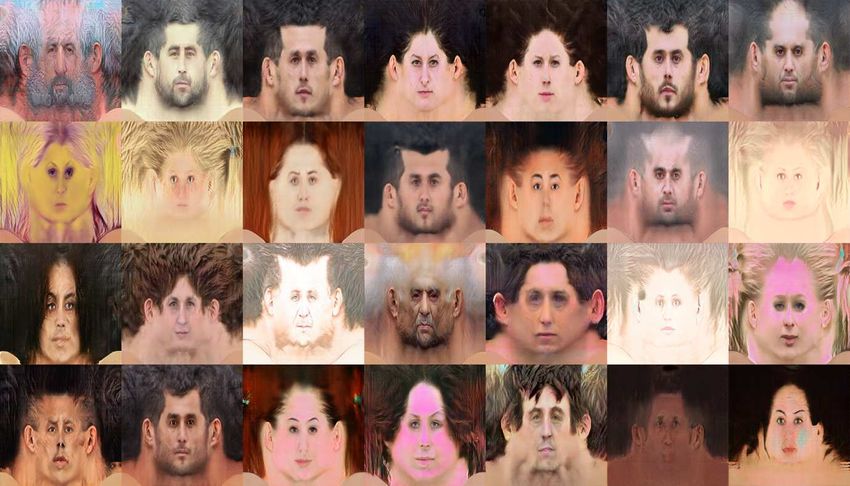
Abstract

Generative adversarial network (GAN), an aspiring area in the field of deep learning,
has made it possible to generate realistic images of human faces, change the style of an
image and generate voice and texts. Generation of realistic images using GANs is an
interesting research area and in this thesis that is the main concern.
     Textures are an important part in creating 3D models and face textures are integral in
creating 3D human models. Generating face textures from 3D scans of faces is already
a known method. But due to its complexity, an endeavour is made in this thesis to
leverage the state of the art generative network to generate good quality textures that
can be efficiently fitted on an available 3D face model. Developing a method to perform
selective modifications on generated face textures and developing an efficient method of
fitting a texture to a 3D model is discussed in this thesis as well.
     As already mentioned generation of textures is not the only concern here. To assure
the diversity of the generated images a face attribute predictor is trained that assures
the diversity of generated images. It is shown that method like regression can prove very
efficient in identifying and changing specific facial features without changing any other
facial properties. Two new indices, the face index and intercanthal index, are proposed
that helps in an accurate geometrical analysis of the generated faces and textures. Post
texture generation, it is shown how efficiently the textures can be fitted on a 3D model
even without any UV map (2D mesh of a 3D model) information (like the different
co-ordinates of the eyes, lips, nose and other facial features). It is shown how a simple
and efficient Support Vector Machine (SVM) technique can be used to align and fit a
2D texture onto a 3D model efficiently. In this thesis, effect of texture augmentations
in training generative networks is also discussed.
     Index Terms- generative adversarial networks, 2D face textures, texture modification,
UV mapping, texture rectification.

                                             i
Contents

1 Introduction                                                                                                                                     1
  1.1 Motivation . . . . . .   .   .   .   .   .   .   .   .   .   .   .   .   .   .   .   .   .   .   .   .   .   .   .   .   .   .   .   .   .   1
  1.2 Problem Description      .   .   .   .   .   .   .   .   .   .   .   .   .   .   .   .   .   .   .   .   .   .   .   .   .   .   .   .   .   2
  1.3 Contribution . . . . .   .   .   .   .   .   .   .   .   .   .   .   .   .   .   .   .   .   .   .   .   .   .   .   .   .   .   .   .   .   2
  1.4 Structure . . . . . .    .   .   .   .   .   .   .   .   .   .   .   .   .   .   .   .   .   .   .   .   .   .   .   .   .   .   .   .   .   3

2 Background                                                                                                                                        5
  2.1 Linear Regression . . . . . . . . . . . . . . . . . . .                                      .   .   .   .   .   .   .   .   .   .   .   .    5
  2.2 Support Vector Machine . . . . . . . . . . . . . . .                                         .   .   .   .   .   .   .   .   .   .   .   .    6
  2.3 Convolutional Neural Networks (CNN) . . . . . . .                                            .   .   .   .   .   .   .   .   .   .   .   .    7
      2.3.1 Convlution Operation . . . . . . . . . . . .                                           .   .   .   .   .   .   .   .   .   .   .   .    8
      2.3.2 Non-linearity /Activation Function . . . . .                                           .   .   .   .   .   .   .   .   .   .   .   .    9
      2.3.3 Pooling or Subsampling operation . . . . . .                                           .   .   .   .   .   .   .   .   .   .   .   .   10
      2.3.4 Fully Connected Layer . . . . . . . . . . . .                                          .   .   .   .   .   .   .   .   .   .   .   .   10
      2.3.5 Training the network using backpropagation                                             .   .   .   .   .   .   .   .   .   .   .   .   10
  2.4 General Overview of Generative models . . . . . . .                                          .   .   .   .   .   .   .   .   .   .   .   .   11
  2.5 Generative Networks . . . . . . . . . . . . . . . . .                                        .   .   .   .   .   .   .   .   .   .   .   .   13
      2.5.1 Generative Adversarial Network (GAN) . . .                                             .   .   .   .   .   .   .   .   .   .   .   .   13
  2.6 StyleGAN architecture . . . . . . . . . . . . . . . .                                        .   .   .   .   .   .   .   .   .   .   .   .   15
      2.6.1 State of the Art GAN Model (StyleGAN) .                                                .   .   .   .   .   .   .   .   .   .   .   .   15
  2.7 Face Landmark Detection . . . . . . . . . . . . . .                                          .   .   .   .   .   .   .   .   .   .   .   .   18
  2.8 3D model and UV mapping . . . . . . . . . . . . .                                            .   .   .   .   .   .   .   .   .   .   .   .   19

3 Related Work                                                                                                                                     21
  3.1 Generative Adversarial Networks                      .   .   .   .   .   .   .   .   .   .   .   .   .   .   .   .   .   .   .   .   .   .   21
  3.2 Evaluating GAN output . . . . .                      .   .   .   .   .   .   .   .   .   .   .   .   .   .   .   .   .   .   .   .   .   .   23
  3.3 Image Data Modification . . . . .                    .   .   .   .   .   .   .   .   .   .   .   .   .   .   .   .   .   .   .   .   .   .   24
  3.4 Face Texture Generation . . . . .                    .   .   .   .   .   .   .   .   .   .   .   .   .   .   .   .   .   .   .   .   .   .   25

                                                       iii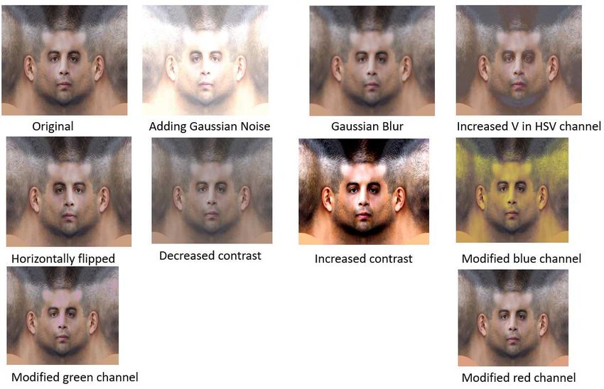
Contents

4 Methodology                                                                                                27
  4.1 Dataset Preparation . . . . . . . . . . . . . . . . . . .      .   .   .   .   .   .   .   .   .   .   27
      4.1.1 CelebFaces Attributes Dataset (CelebA) . . . .           .   .   .   .   .   .   .   .   .   .   27
      4.1.2 Texture Dataset . . . . . . . . . . . . . . . . . .      .   .   .   .   .   .   .   .   .   .   28
  4.2 Training . . . . . . . . . . . . . . . . . . . . . . . . . .   .   .   .   .   .   .   .   .   .   .   29
      4.2.1 Effect of image augmentation during training .           .   .   .   .   .   .   .   .   .   .   31
  4.3 Degree of Realism Assessment . . . . . . . . . . . . . .       .   .   .   .   .   .   .   .   .   .   32
  4.4 Modification of Generated Images (Faces and Textures)          .   .   .   .   .   .   .   .   .   .   35
      4.4.1 Style mixing using the StyleGAN model . . . .            .   .   .   .   .   .   .   .   .   .   36
      4.4.2 Modification using Regression . . . . . . . . . .        .   .   .   .   .   .   .   .   .   .   36
  4.5 Best Fit Texture Resolution . . . . . . . . . . . . . . .      .   .   .   .   .   .   .   .   .   .   40
  4.6 Rectifying Bad Fit Textures . . . . . . . . . . . . . . .      .   .   .   .   .   .   .   .   .   .   42

5 Results and Discussion                                                                                     47
  5.1 Training of the StyleGAN architecture . . . . . . . . . .          .   .   .   .   .   .   .   .   .   47
      5.1.1 Evaluating Training progress using FID score . .             .   .   .   .   .   .   .   .   .   47
      5.1.2 Degree of Realism for generated faces . . . . . . .          .   .   .   .   .   .   .   .   .   48
  5.2 Variational Analysis . . . . . . . . . . . . . . . . . . . .       .   .   .   .   .   .   .   .   .   50
  5.3 Finetuning with Texture . . . . . . . . . . . . . . . . . .        .   .   .   .   .   .   .   .   .   51
  5.4 Modification of Generated Textures . . . . . . . . . . . .         .   .   .   .   .   .   .   .   .   54
      5.4.1 Style mixing implementation for textures . . . . .           .   .   .   .   .   .   .   .   .   54
      5.4.2 Modification of Images using Regression Analysis             .   .   .   .   .   .   .   .   .   56
  5.5 Determining the best fit texture for the 3D face model .           .   .   .   .   .   .   .   .   .   61
  5.6 Rectification of distorted texture . . . . . . . . . . . . .       .   .   .   .   .   .   .   .   .   65

6 Conclusion and Outlook                                                               67
  6.1 Conclusion . . . . . . . . . . . . . . . . . . . . . . . . . . . . . . . . . . . 67
  6.2 Future Work . . . . . . . . . . . . . . . . . . . . . . . . . . . . . . . . . . 68

References                                                                                                   69

                                           iv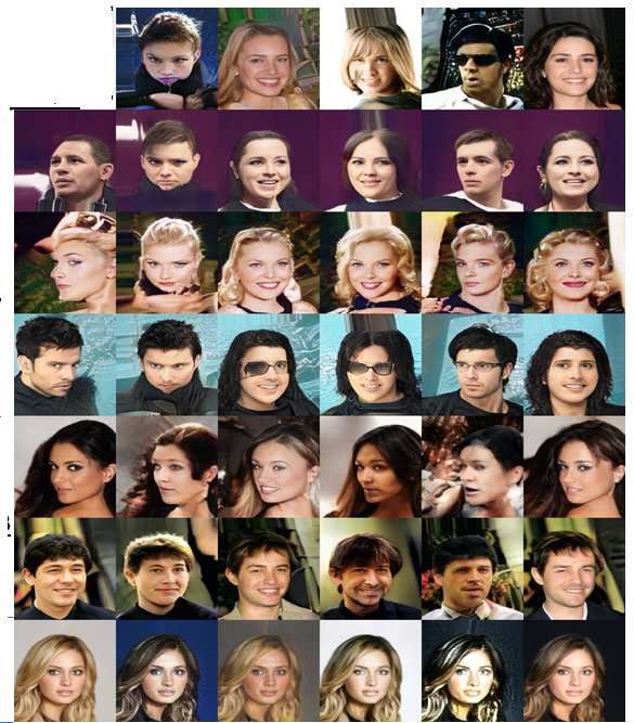
1
                                                             Introduction

1.1     Motivation
Synthetic data is a crucial asset in the field of machine learning. In the field of au-
tonomous driving the use of synthetic or artificial data is significant. An autonomous
driving system needs to be trained using a simulation environment because using real
data is not always a practical solution. The simulation environment consists of buildings,
cars, signal posts, pedestrians, etc. In order to train a system to be robust and reliable,
it needs to be trained with a lot of variations, so that the system is prepared to face
any kind of situation. One of the important components in the simulation environment
are the pedestrians and creating these pedestrians involves 3D models and 2D textures
[Figure: 1.1(a)].
    Creating 2D textures e.g. for faces using the conventional methods of obtaining 3D
scans and extracting texture using some complex mathematical process leads to inferior
quality textures [Figure: 1.1(b)]. And in order to bring variations there should be more
3D scans and hence the entire process is inefficient and time consuming. Textures are
also manually designed by designers. Although these manually designed textures are of
good quality, it is still very time consuming.
    Based on the above-mentioned facts an endeavour is made in this thesis to automate
this texture generation process for pedestrian modelling in simulation environments. By
automating this process more high-quality textures with variations can be generated
in significantly less amount of time, than that could be done using the conventional
methods.
    This approach might also prove beneficial for designing computer games. The use
of human figures in computer games is extensive and if this texture generation can
be automated then it will be possible to generate different figures in significantly less
amount of time. Another important application is training of face recognition systems.
Generating face textures with a lot of variations which could then be wrapped around
a 3D model to create a face [Figure: 1.1(a)], will help in training the face recognition
system, making the surveillance system more robust and reliable and will simultaneously
reduce the effort of collecting photographs of different faces required for the training.

                                            1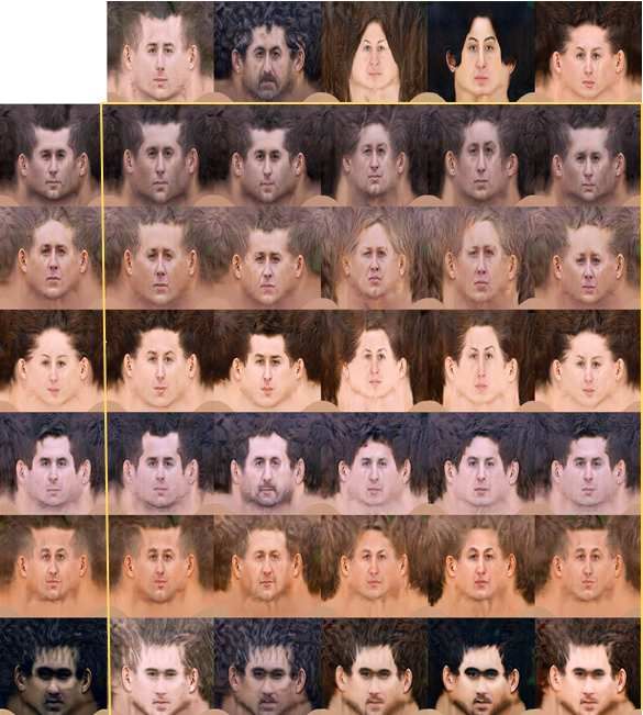
1. Introduction

 3D Model        2D UV Map       UV mapping
                                 in Blender

  Generative Generate                                       3D scan of   Face texture obtained from
  network                               Model of face       face         3D scans

                        2D Texture
                         (a)                                                    (b)

Figure 1.1: (a)Creating a face model using 3D model and 2D texture generated using a
generative network; (b)3D scan and textures generated from 3D scans.

    Automating the generation of textures is possible leveraging the recent development
in the field of deep learning in the form of generative networks (explained in Background
chapter). With the help of generative networks, it is possible to create high quality
textures with substantial amount of variations and that too without obtaining any 3D
scans or doing any manual design.
    Hence, this thesis provides a proof of concept on how this generation, creating vari-
ations and fitting of 2D textures could be automated.

1.2       Problem Description
The basic idea is demonstrated in figure 1.1(a) where a model of a face is created using
a 3D model and 2D texture. The purpose of the thesis is generation of 2D textures for
3D modelling of the pedestrian models (human figures) using deep learning techniques.
Here the main concern has been the generation and fitting of face textures. This involves
the 2D face texture generation, performing quality checks to assess the realism of the
generated textures, making sure that the generated textures are quite diverse in nature,
wrapping of the 2D face textures on a 3D face model, assessing the quality of the face
after the 2D texture being wrapped on it and in case of distortions after the wrapping
step, finding a solution for it. The figure 1.2 gives an overview for the workflow of the
thesis.

1.3       Contribution
The main contributions in the thesis can be summarized in the following points:

   • The effect of data augmentation while training GAN architecture is analysed.

                                                        2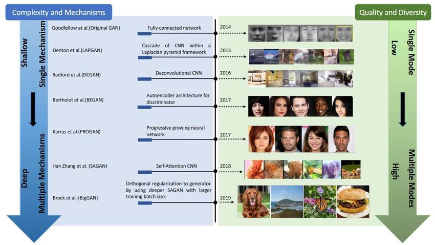
1. Introduction

   • Variational analysis is performed on the generated textures to make sure the gen-
     erated textures are diverse in nature.
   • Degree of realism is calculated for the assessment of the generated textures. Two
     new metrics are introduced apart from the conventional Frechet Inception Distance
     (FID) score. The two new metrics are Intercanthal Index and Face Index which
     are described in the Methodology chapter.
   • StyleGAN’s style-mixing method is implemented on the generated 2D face textures
     to produce random variations on the textures.
   • The concept of linear regression and vector orthogonalization is used to implement
     conditional variation on the generated textures.
   • The generated 2D face textures are then fitted on the 3D model using the concept
     of UV mapping.
   • The texture wrapped 3D model is analysed for distortions or irregularities.
   • Experiments are performed to separate bad textures (those that causes distortions
     after wrapping on the 3D model) and acceptable textures.
   • Support Vector machine (SVM) is implemented to classify acceptable textures and
     bad textures. And last but not the least, the bad textures are converted to the
     acceptable ones leveraging the SVM implementation that is described in details in
     the Methodology chapter.

1.4     Structure
The thesis is divided into the following sections:
   • The Background chapter explains the different concepts that are used for the suc-
     cessful completion of the thesis. The topics that are discussed are Linear Regres-
     sion, Support Vector Machine, Convolutional Neural Networks (CNN), Generative
     Networks, Support Vector Machines (SVM), and last but not the least UV Map-
     ping.
   • The Related Work chapter tries to give an overview of the different researches that
     have been done, which are relevant to the thesis. Related works in the field of
     GAN architecture, texture generation and generated image modifications.
   • The Methodology chapter describes the main contributions of the thesis in details,
     the ones that are being described in the Contribution section above.
   • The Results and Discussion chapter summarizes the different evaluations that has
     been performed during the thesis, like the variational analysis of the generated
     textures, degree of realism assessment, effect of data augmentation during GAN
     training, etc. The above mentioned topics in the Contribution section is actually
     divided between the Methodology and Results and Discussion chapter, where the
     Methodology chapter describes the methods that have been implemented and the
     Results and Discussion chapter summarizes the different outcomes of the methods
     that are being implemented. It keeps the thesis structure clean and tidy.
   • Last but not the least the Conclusion chapter gives an overview of the entire thesis
     and the final outcome and also throws some light on the possible future areas of

                                            3
1. Introduction

     research building on this work.

                    Variational                           Variational                    Style-
        Train       Analysis               Retrain        Analysis      Modification
                                                                                         mixing      Wrapping
        StyleGAN                           StyleGAN                     of textures                  texture on
        on CelebA                          for textures                                              3D model
                    Degree                                 Degree                       Regression
                    of Realism                             of Realism                   method
                    test                                   test

                             Test the                     Rectify bad   Classify       Check for
                                           Wrap the                                                  Determine
                             new wrapped                  textures      good vs bad    distortion
                                           rectified                                                 the best fit
                             textures                     with SVM      textures       on wrapped
                                           texture                                                   resolution
                                                                                       textures

                                  Figure 1.2: The workflow of the thesis

                                                          4
2
Background
The purpose of this chapter is to explain the different concepts that is used throughout
this thesis, for better understanding of this thesis. This chapter is divided into six parts.
• Section 2.1 explains Linear Regression, which is basic machine learning.
• In section 2.2 the concept of Support Vector Machine is explained.
• Section 2.3 explains Convolutional Neural Networks (CNN) which is an itergral
part of deep learning.
• Section 2.4 and 2.5 explains Generative Networks in General that is the building
block of the thesis.
• Section 2.6 describes the State of the art architecture for GAN i.e. the StyleGAN
architecture.
• In section 2.7 face landmark detection is discussed using dlib face landmark de-
tector.
• Section 2.8 explains the process of fitting of a 2D texture on a 3D model.
2.1 Linear Regression
One of the very basic concept that is used in the thesis is Linear Regression for the
conditional modification of fake images, which is explained in the Own Work chapter.
Linear regression is a linear approach that models the relationship between dependent
and independent variables. Given a data yi , xi1 , ..., xip , where y is the dependent variable
and xi1 , ..., xip is a p dimensional vector, which is the independent variable. The variable
X which is a p dimensional vector is called the regressor variable. The model takes the
form:
yi = b0 + b1 xi1 + .... + bp xip = Xi | b (2.1)
Here,
• y is response vector of length n.
• X is an n x (p + 1) matrix of independent variables.
• b is a (p + 1) vector of regression coefficients.
52. Background
This kind of linear regression i.e. represented by [Eq: 2.1], is known as multiple linear
regression, also known as multivariate linear regression.
The image [Figure: 2.1] gives a geometrical interpretation of Linear Regression. The
basic idea of Linear Regression is about fitting a straight line through the data-points.
21
Line Fit: y=b0 + b1 .X
20
19
18
Y 17
16
15
14
13
12
-3 -2 -1 0 1 2 3
X
Figure 2.1: Scatter plot for linear regression. The best values of b approximates the best fit
line.
2.2 Support Vector Machine
A Support Vector Machine (SVM) is a discriminative classifier that is defined by separat-
ing boundary or hyperplane. Given a labelled training data, SVM outputs a boundary,
which is H0 in figure 2.2, which categorizes new examples. The name support vector
machine comes from the support vectors that lie closest to the decision surface(or hy-
perplane), the red and the green dots that lie on the lines H1 and H2 [Figure: 2.2]
are the support vectors and these are the data-points that are most difficult to classify.
Another interpretation for SVM can be that it maximizes the margin around the sep-
arating hyperplane. The d in figure 2.2 is the margin of separation, i.e. the separation
between the hyperplane and the support vector for a given weight vector w and bias b.
The input to the SVM is a set of input/output training pair samples (the input sample
features x1 , x2 , ..., x3 and the output result y ). The SVM outputs a set of weights w, one
for each feature, whose linear combination predicts the value of y. From figure 2.2 the
separating hyperplane is H0 defined by the equation w.x + b = 0, where w is the weight
vector, x is the input vector and b is the bias. In order to maximize the margin, i.e. the
distance 2d, ||w|| has to be minimized with the condition that there are no datapoints
between H1 and H2 [Equation: 2.2, 2.3]:
xi .w + b ≥ +1 when yi = +1 (2.2)
xi .w + b ≤ −1 when yi = −1 (2.3)
62. Background
H1
H0
H2 d+
d-
w.x+b=+1
w.x+b=0
w.x+b=-1
Figure 2.2: Support Vector Machine overview
2.3 Convolutional Neural Networks (CNN)
A CNN is a deep learning algorithm that takes in an input image and assign various
aspects/objects in the image and is capable of differentiating an image based on some
predefined classes. A CNN gets its name from the type of hidden layers present in
it. A CNN consists of convolutional layers, pooling layers, fully connected layers, and
normalization layers.
To mention a little bit of history, the very first CNN architecture was LeNet, which
was a pioneering work by Yann LeCun (1988) [LBBH98], which helped to gear up the
field of deep learning. Below is an image that gives an intuitive idea about how the
CNN architecture works.
Convolution+ReLU Pooling Convolution+ReLU Pooling Fully Connected
Layer
Dog (0.01)
Input Image
Cat (0.04)
Boat (0.94)
Bird (0.01)
LeNet Architecture
Figure 2.3: A simple CNN architecture [LBBH98]
This CNN architecture[Fig: 2.3] classifies the image into 4 classes namely the dog,
cat, boat and bird. It is evident from the picture that boat gets the highest probability.
Though just saying it seems to be a lot more intuitive, there is some serious mathematics
that goes behind such architectures. There are 4 main operations that are being carried
out in the CNN architecture:
1. Convolution.
72. Background
2. Activation Function (Non Linearity like ReLU).
3. Pooling or Subsampling.
4. Classification (Fully Connected Layer)
These operations are basic to all classes of neural networks and hence understanding
them is key to understanding the Thesis properly.
Now we all know that image is a matrix of pixel values. Channel of a image is
referred to as the number of colour elements that the image has. An image from a
standard digital camera will have 3 channels namely Red, Green and Blue. A gray
scale image is an image with only a single colour channel. The pixel values are between
0 and 255. Hence these channels are also known as the 8 bit colour channels.
2.3.1 Convlution Operation
1 1 1 0 1 1 1 1 0 1 1 1 1 0 1
1 0 1 1 1 1 0 1 1 1 1 0 1 1 1
0 1 1 0 1 0 1 1 0 1 0 1 1 0 1
1 0 0 1 1 1 0 0 1 1 1 0 0 1 1
0 1 1 1 0 0 1 1 1 0 0 1 1 1 0
5x5 Image Convolution operation Convolution operation
performed on the image performed on the image
using the 3x3 Filter matrix. using the 3x3 Filter matrix.
1 1 1 4 4 3
1 0 1
0 1 1
3x3 Filter Convolved Feature Convolved Feature
Figure 2.4: (Left to right) Explanation of the convolution operation.
ConvNets (convolution network) derive their name from convolutional operator. The
basic purpose of the convolution is extracting features from the input image. Convolu-
tion preserves the spatial relationship between pixels by learning image features using
small squares of input data.
As it is already mentioned that image is a matrix values, let us take an image matrix
of 5x5 image pixel values are only 0 and 1 (first figure from top left )[Figure: 2.4].
The small 3x3 matrix (first figure from bottom left) [Figure: 2.4] is also called the
Kernel or Filter. The filter is slid over the 5x5 image matrix and multiplication is
performed with the elements in the 3x3 matrix with elements of the 5x5 image matrix,
over the block on which the filter is superimposed as marked by the yellow block (top
middle from left)[Figure: 2.4]. The multiplication is followed by addition of the results
82. Background
of multiplication of each individual cell in the block. Hence convolution is a purely linear
operation. The convolution operation can be summarized by the following equation:
XX
G[m, n] = (f ∗ h)[m, n] = h[j, k]f [m − j, n − k] (2.4)
j k
here f is the input image and h is the kernel. The indices of the rows and columns
of the resultant matrix are marked with m and n respectively. Here in figure 2.4, it is
evident that the kernel has moved one distance, and this is known as the stride. Here
stride is 1. The matrix formed after convolution is known as the Feature Map (bottom
middle figure from left)[Figure: 2.4]. The number of feature maps obtained depends on
the number of filters used for convolution. It is important to mention the filters acts as
feature detectors for the original input image. The spatial size of the output volume of
the feature maps can be calculated by the following formula:
W − K + 2p
F eature map volume = +1 (2.5)
S
where W is the input feature (image) volume size (e.g. W = 5 from figure 2.4), the
kernel field size of the convolutional layer neurons is denoted by K, S denotes the stride
that is applied (in the above case 1) and the amount of zero padding if used on the
border is denoted by p.
2.3.2 Non-linearity /Activation Function
The output of a neuron is basically a liner operation that can be summarized by the
formula Output = (weight·input)+constant, where Output is the neuron output, input
is the input to the neuron, weight defines the strength of the connection between input
and output neuron and the constant is also known as the bias term in machine learning.
The output can range between −∞ to +∞. The neuron is unaware of the bounds of
the value. Hence in order to decide whether the neuron will be activated or not, the
purpose of the activation function comes into play, where the output of the neuron is
bound between certain values and at the same time the activation function introduces
non-linearity to the model. There are many different kinds of activation functions like
the Step, Sigmoid, Tanh, ReLU, etc. Among them ReLU activation function is one of
the most commonly used.
The ReLU or Rectified Linear Unit[Aga18] is an activation function. Since most of
the data in real world is non linear in nature, it is the job of the activation function to
introduce non-linearity in the model, otherwise it is just a simple linear operation (i.e
convolution). ReLU can be described as A(x) = max(0, x), where A defines the ReLU
operation and x is the neuron output. The ReLU is not bound, though it is a good
approximator. The range of ReLU is [0, ∞]. ReLU is an element wise operation and
removes all the non zero values from the convoluted matrix or feature map and in doing
so technically it removes sharp edges from the convoluted image.
92. Background
2.3.3 Pooling or Subsampling operation
Pooling is also known as subsampling/downsampling or spatial pooling. Spatial pooling
can be different types: max, average, etc.
In case of max pooling a spatial neighbourhood (e.g 2x2 ) window is defined and
the largest element from the rectified feature map within that window is taken. Instead
of taking the largest element, the average of all the elements in that window can be
considered, which in that case will be known as average pooling. An example of max
pooling operation with a spatial window of 2x2 on a rectified feature map is shown
below:
x
1 1 2 4
5 6 7 8 6 8
3 2 1 0 Max pool with 3 4
2x2 filters
1 2 3 4 and stride 2
y
Rectified Feture Map
Figure 2.5: Max Pooling operation
We slide the window 2x2 by 2 cells and take the maximum value in each region. The
Max Pooling serves some important functions:
1. As it is evident from figure 2.5 that it reduces the dimensionality of the rectified
feature map. Hence it makes input more manageable.
2. Reduces the number of parameters and computations and in a way controls over-
fitting.
3. Makes the network invariant to small transformations and distortions.
4. Makes the network scale invariant. This is very useful because in real life we may
have the image of same thing but with different scales.
2.3.4 Fully Connected Layer
The Fully Connected layer is the classical neural network architecture, in which all
neurons connect to all neurons in the next layer.
The rectified feature maps i.e the outputs from the Convolution and pooling layers
serves as high-level features of the input image and the fully connected layer use these
features for classifying the input image into various classes.
2.3.5 Training the network using backpropagation
The overall training process of the CNN can be summarized as follows:
102. Background
• Step 1: First of all we initialize all the filters with random Gaussian values. It is
advised that the initialization should not be done with all zeros.
• Step 2: The input to the network is training image of size N xN , that goes
through all the convolution, pooling and fully connected layers and finds out the
output probabilities for each class. (E.g.: In our above example we have 4 classes
and we can think of an output such as [0.2,0.3,0.4,0.1]). Since the filter weights
are randomly assigned, for the 1st training example, output probabilities are also
random.
• Step 3: The error is calculated as follows:
s
PT 2
i=1 (P redictedo/p − Actualo/p )
T otal Error(loss) = (2.6)
T
Here the mean squared error(MSE) loss has been used for the example where T is
the number of classes. Here P redictedo/p is the output predicted or calculated by
the network and Actualo/p is the actual reference output provided beforehand.
• Step 4 : The next step is to reduce the loss by performing optimization on the
loss function. This is done using the backpropagation method. The backprop-
agation method is is used to calculate the gradients of the loss function w.r.t the
network parameters and then uses gradient descent to update all the parameter
values to minimize the loss.
– The weights are adjusted proportionally to their error contribution.
– When the same input image is again fed to the network then output may
become [0.1,0.1,0.7,0.1]. This clearly shows that the output indicating to a
particular class.
– This proves that the network has learned to classify something. And this
process continues until and unless we are satisfied with the loss minimization.
2.4 General Overview of Generative models
Generative models are a special branch of machine learning models that are used to
generate data. In other words, generative models can generate data that we feed them
as training data.
The different types of generative models are:
• Autoencoders: An autoencoder is a type of model that is used to learn low level
representation or embeddings of the training data. It is generally used to mimic
the input data to the output. The autoencoder maily consists of 4 parts namely the
encoder, bottleneck, decoder and reconstruction loss. The encoder model
helps in learning the lower dimensional representation of the input data. The
bottleneck is the layer that contains the compressed representation. The decoder
112. Background
is the network that helps in reconstruction of the original data from the compressed
one and the reconstruction loss is the method that gives the intuition of how well
the autoencoder is performing. The main benefit of an autoencoder network is
dimensionality reduction. There are different variations of autoencoders present
like the variational autoencoders[KW19]. A variational autoencoder is a type of
autoencoder whose training is regularized to avoid overfitting and to make sure
that the latent space or the bottleneck layer representation has good properties
that enable generative process which means new content can be generated which
was not possible in case of a simple autoencoder.
Encoder
Decoder
Bottleneck
Output Layer
Input Layer
Latent Code
x x'
(h)
Figure 2.6: Schema of basic Autoencoder. The Input Layer represents training data.
Latent Code represents the intermediate vector or the embedding of the input X. The En-
coder network maps the input x to intermediate state Latent Code and the Decoder network
maps Latent Code to X 0 .
• Generative Adversarial Networks (GANs): The GAN architecture has a
generator model q(x/h) to map the intermediate state of h represented in figure
2.6 to the input space X. And there is a discriminative model p(y/x), which tries
to associate an input instance x to a yes/no binary answer y, about whether the
generator model generated the input or was a genuine sample from the dataset we
were training on. Some of the notable GAN architectures are the DCGAN[rad],
PROGAN[KALL17], StyleGAN[KLA18]. The workflow is represented by figure
2.7.
• Auto-regressive models (AR): Autoregressive models predicts the future be-
haviour based on the past behaviour.
Autoregressive models like PixelRNN[vdOKK16], trains a network that models
the conditional distribution of each and every individual pixel, given the previous
pixel. In AR model, the value of the outcome variable Y at some instance of time
t is directly related to the predictor variable X. The difference between simple
linear regression and AR models is that Y is dependent on X and previous values
for Y .
122. Background
2.5 Generative Networks
After the elaborate introduction of CNN, this section will generally involve the ex-
planation of Generative Networks. Till date there has been tremendous improvement
in the field of discriminative models, that generally map high dimensional inputs to
class labels. These successes is mainly based on the backpropagation and dropout al-
gorithms, using piece-wise linear units which have a particularly well behaved gradient.
Deep generative networks have had a less impact, because of the difficulty of approxi-
mating many intractable probabilistic computations that arise in maximum likelihood
estimation and related strategies, and due to the difficulty of leveraging the benefits of
piece-wise linear units in the generative context. This problem was addressed by Ian
Goodfellow and his team in the year 2014, by the introduction of Generative Adversarial
Networks[GPAM+ 14].
2.5.1 Generative Adversarial Network (GAN)
Generative vs. Discriminative Algorithms
To understand GAN architecture it is very important to understand the difference be-
tween Generative and Discriminative algorithms.
Discriminative algorithms tries to map a high dimensional input to a class. Hence
basically it is solving a classification problem. In mathematical terms it can be repre-
sented as p(y|x). Here y is the class variable and x is the feature variable. For example
given the properties of an email what is the probability that the email is spam or not.
The question that the generative model tries to answer, is that assuming the email is
spam, how likely are the features? While discrminative models care about the relation
between x and y, generative models care about how to get x.
The GAN Framework
In the GAN architecture there are two CNNs competing against one another. One is
known as the generator and the other is known as the discriminator. In simple
language, the generator generates new data instances while the discriminator evaluates
them for authenticity. The discriminator decides whether the data instances fed to it is
sampled from the real data or generated by the generator.
The discriminator and generator are represented by 2 functions (in this case neural
networks) that are both differentiable w.r.t their parameters and input. The discrimi-
nator takes input x(from the real data) and it’s parameters are ΘD . The generator is
defined as G and it takes input z (array of random numbers) and it takes ΘG as it’s
parameters.
Both D the discriminator and G the generator have cost functions that are defined
w.r.t their parameters. The D minimizes J D (ΘG , ΘD ) by controlling ΘD and the G
minimizes J G (ΘG , ΘD ) by controlling only ΘG . Here J() is the cost function or loss
function used to optimize the generator and the discriminator network.
132. Background
As the cost functions depends on each others parameters, this scenario represents
more of a game than a optimization problem. The solution of a game is finding the
NASH equilibrium, which is a tuple (ΘD , ΘG ), where ΘG is the local minimum for G
parameters and ΘD is the local minimum for D parameters.
D(x) tries D tries to make
to be near 1 D(G(z)) near 0,
G tries to make
D(G(z)) near 1
Differentiable
function D
D
x sampled
from data x sampled from
model
Differentiable
function G
Input noise z
Figure 2.7: The GAN framework represents two adversaries namely Discriminator (D) and
Generator(G). Typically D and G is represented by deep neural networks. There are 2 scenarios
in this game play. Firstly the D is fed with real training sample x and D returns the probability
that it’s output is real rather than fake. The goal of D is to make D(x) close to 1. Secondly,
G is fed an array of random numbers z that may be sampled from a Gaussian distribution. D
is then fed with G(z) and here both D and G works together. D tries to make D(G(z)) close
to 0 while G tries to make the same quantity close to 1.
Cost function: D and G play the following two-player minimax game with value
function V (G, D):
minG maxD V (G, D) = Σx∼pdata (x) [logD(x)] + Σz∼pz (z) [log(1 − D(G(z))] (2.7)
Here pdata (x) is the data distribution from which the original data is sampled and pz (z)
is the distribution from which the latent vector (noise) is sampled that is fed to the
generator G. x is the original data or the image in this case and z is the latent or noise
vector that is fed to the generator.
142. Background
Real Image x
D Cost
Discriminator
Generator
Figure 2.8: GAN loss function [GPAM+ 14]. D() is the discriminator, G() is the generator,
m are the total number of samples, x and z is the real image and the latent vector respectively.
2.6 StyleGAN architecture
2.6.1 State of the Art GAN Model (StyleGAN)
The GAN model that is used for this thesis is the StyleGAN architecture[KLA18]. Until
now most of the improvements to the GAN network has been done on Discriminator
models. But the Style Generative Adversarial Network, or StyleGAN in short, is an
extension to the GAN architecture that proposes a new generator architecture. The
architecture includes a fully connected mapping network, to map the noise vector to an
intermediate latent space. The intermediate latent space is used to control style at each
point in the generator model, and the introduction to noise as a source of variation at
each point in the generator model.
152. Background
Generator
Normalize Noise
Synthesis network g Training
Mapping Const 4 x 4 x 512
Network f + B
Random Vector A AdaIN
(Latent Code) FC Conv 3 x 3
+ B ProGAN
FC AdaIN Discriminator
A
FC 4x4
FC Umsample
1024 x 1024
Conv 3 x 3
FC
512 x 1
Loss
+ B
4x4
FC A AdaIN ... (WGAN-GP)
Conv 3 x 3
FC
+ B
FC A AdaIN
8x8
...
w W
1024 x 1024 Training
Real Sample
Downscaling
Figure 2.9: Overview of the StyleGAN network
Style-based generator
Traditionally the latent code i.e. the noise vector is directly applied to the input layer.
In case of StyleGAN, the entire input layer is omitted and instead starts from a learned
constant [Figure: 2.9]. Given a latent code z in the input latent space Z, a fully
connected mapping network (non-linear in nature) f : Z → W first produces w ∈ W .
The dimensionality of the latent code z and the dimensionality of the latent space w is
the same. The mapping network f is 8-layer fully connected network.
The A represents learned affine transformation. The learned affine transformation
transforms w to styles y = (ys , yb ), that controls the AdaIN operation[KLA18, HB17].
AdaIN refers to "Adaptive Instance Normalization" and it is defined as:
xi − µ(xi )
AdaIN (xi , y) = ys ,i + yb ,i (2.8)
σ(xi )
where xi refers to feature map, µ(xi ) is the mean of xi and σ(xi ) is the standard deviation
of xi . xi is normalized separately and then biased and scaled using the learned affine
162. Background
transformations performed in block A. Hence the dimensionality of y is twice the number
of feature maps on that layer.
Last but not the least, the generator is provided with explicit noise inputs, repre-
sented by block B. These are single-channel images consisting of uncorrelated Gaussian
noise, and a dedicated noise image is fed to each layer of the synthesis network. The
noise image is broadcasted to all the feature maps using learned per feature scaling
factors and then added to the output of the corresponding convolution.
Properties of Style-based generator
• The generator architecture makes it possible to control the image synthesis via a
scale-specific modifications to the styles.
• A concept of mixing regularization is employed where a given set of images is
generated using two latent codes z1 and z2 and as a consequence there are w1 and
w2 that control the styles. This technique prevents the network from assuming
that adjacent styles are correlated.
• Stochasticity in an image refers to the placement of hairs, skin pores, etc. This
stochasiticity is achieved by adding per pixel noise after each convolution, that is
evident from figure 2.9. In the figure that is represented by block B.
• The changes in stochastic variation does not have any global effects. The style
affects the entire image. Global effects like pose, lighting, etc are completely
controlled by the styles, whereas the noise is added independently of each other.
If the network would have tried to control the global effects using the noise, then
that would be penalized by the discriminator.
• One of the most important concept that has been implemented in the StyleGAN is
the truncation trick in w. Here the generator truncates the intermediate vector w,
to keep it close to the average intermediate vector to avoid generating poor images.
The concept is quite simple, instead of using the intermediate vector directly, w is
transformed to
wnew = wavg + ψ(w − wavg ) (2.9)
where ψ defines the standard deviation, i.e how far the generated image can be
from the average image. wavg is produced by selecting many inputs and then
taking their intermediate vector using the mapping network and then taking their
average.
Loss function
The loss function that is used for the purpose of StyleGAN is the Wasserstein Loss[ACB17].
The Wasserstein Distance (also known as the Earth Mover Distance) is actually the min-
imum cost of transporting mass to convert a data distribution q to p. The Wasserstein
172. Background
distance is defined as
W (Pr , Pθ ) = sup Ex∼Pr [f (x)] − Ex∼Pθ [f (x)] (2.10)
where,
• f is 1-Lipschitz function, such that |f (x1 ) − f (x2 )| ≤ |x1 − x2 |.
• ||f || ≤ 1
• sup − > Least upper bound.
• Pr and Pθ are two different probability distributions.
The figure 2.10 shows the WGAN loss function. Compared to the original GAN algo-
rithm, the WGAN undertakes the following changes:
• After every gradient update on the Discriminator function, the weights are clamped
to a small fixed range [-c,c].
• Use of a new loss function derived from the Wasserstein distance where there is no
more logarithm term. The discriminator model does not act as a critic anymore
but acts as an helper for estimating the Wasserstein metric between real and
generated data distribution.
Real Image x
f Cost
Discriminator
Generator
Figure 2.10: WGAN loss function[ACB17]
2.7 Face Landmark Detection
One of the popularly used face detector is the CNN based face detector from dlib. Dlib
is a toolkit for making the real world machine learning and data analysis applications
in C++. Although, it is written in C++, it has good, easy to use python bindings. The
facial landmark detection is generally used for this thesis.
This detector is based on the Histogram of oriented gradients and linear SVM.
While the HOG+SVM based face detector works perfectly fine, there is also CNN based
182. Background
dlib face detector. The HOG based face detector in dlib is meant to be a good frontal face
detector. Meanwhile the CNN based detector is capable of detecting faces in almost all
angles. But CNN based detection is computationally expensive. Hence, for the purpose
of this thesis the HOG based detector is used because it serves the purpose quite well.
The image [Figure: 2.11] shows an example of the dlib face detector (HOG+SVM based)
on a sample image from CelebA dataset. The Annotated Image gives the bounding box
for the face including the 68 coordinates for the facial landmarks that are marked by
red dots.
Figure 2.11: Dlib face detector applied on an Image
2.8 3D model and UV mapping
One important part of the thesis is to fit the generated face textures on a 3D model
and determine what resolution of texture, fits best on the available 3D model. In order
to fit the 2D texture into a 3D model is called UV mapping[HLS07]. UV mapping is
the 3D modelling process of projecting a 2D image to a 3D model’s surface for texture
mapping. 0 U 0 and 0 V 0 represents the axes of the 2D texture because 0 X 0 , 0 Y 0 and 0 Z 0
are used to denote the coordinates of the 3D object. The figure 2.12 gives an overview
of the UV mapping concept. A UV map consists of the 3D model’s XY Z coordinates
flattened into 2D UV space.
192. Background
(u,v)
Texture Space 2D (x,y)
Screen Space 2D
Object Space or
Parameterization World Space 3D Projection
Figure 2.12: UV mapping overview
The figure 2.13 gives a pictorical representation of the UV mapping concept.
Figure 2.13: The application of a texture in the UV space related to the effect in 3D[HLS07].
203
Related Work
3.1 Generative Adversarial Networks
In the year 2014, Ian J. Goodfellow, for the first time proposed a new framework for
estimating generative models via an adversarial process, in which the generative network
G and the discriminative network D is simultaneously trained. The proposed adversarial
model has a few advantages. Firstly Markov Chains are never needed, and only back-
propagation is used to obtain the gradients, no inference is needed during learning,
and moreover a wide variety of functions can be incorporated into the model. These
aforementioned advantages are primarily computational. There is also some statistical
advantage because the generator network is not directly updated with the data examples,
it is updated only with gradients flowing through the discriminator. The other advantage
of adversarial nets proposed by Goodfellow is that they can represent very sharp, even
degenerate distributions.
There are few other GAN architectures that needs to be mentioned.
Architecture Variant GANs
Many types of GAN variants have been proposed in the architecture, which is summa-
rized in figure 3.2 . These variants have a specific task to perform like image to image
transfer, image super-resolution, image completion and text to image generation. The
architectures mentioned helps in improving the performance of GANs w.r.t to different
scenarios like image quality improvement, image variety improvement, stable training,
etc.
Fully Connected GANs: The original GAN paper[GPAM+ 14] that has been men-
tioned above, uses fully connected layers for generator and discriminator. This archi-
tecture variant has been used to generate simple images of MNIST and CIFAR 10 and
Toronto Face Dataset. It has not shown good generalization performance for complex
image types.
213. Related Work
Laplacian Pyramid of Adversarial Networks (LAPGAN): LAPGAN
architecture [DCSF15] had been proposed to generate high resolution images, from lower
resolution input. LAPGAN utilizes a cascade of CNNs within a Laplacian pyramid
framework to generate high quality images.
Deep Convolutional GAN (DCGAN): It is one of the most important milestones
in the field of GAN architectures. DCGAN[RMC] was the first architecture that applied
a deconvolutional neural network architecture for generator. The DCGAN utilize the
spatial up-sampling ability of the deconvolution operation for generator, which makes
generation of higher resolution images possible. The figure 3.1 shows the architecture of
the DCGAN. Some of the notable features of the DCGAN includes the use of transposed
Figure 3.1: DCGAN generator. A 100 dimensional uniform distribution Z is projected to a
small spatial content convolutional representation with many feature maps. A series of four
fractionally-strided convolutions then convert this high level representation into a 64x64 pixel
image [RMC]
convolution for umsampling and downsampling, use of batch normalization that stabi-
lizes learning by normalizing input at each unit to have zero mean and unit variance
and use of ReLU activation function in the generator and the use of Tanh function at
the output layer of the generator.
Progressive GAN (PROGAN)[KALL17]: This architecture involves the progres-
sive steps towards the expansion of network architecture. It uses the idea of progressive
neural networks. This architecture has the advantage of not forgetting and can take
advantage of the prior knowledge via lateral connections to previously learned features.
Training starts with the low resolution 4x4 pixels images. The generator and the dis-
criminator starts to grow with the training progressing. The progressive nature enables
more stable learning. Current state of the art GAN models are based on this architec-
ture, the most prominent example being the StyleGAN architecture[KLA18], which is
the backbone of the thesis and has been describe in details in the Background chapter.
223. Related Work
BigGAN: BigGAN[BDS18] has also achieved state of the art results. The BigGAN
pulls together the recent best practises in training class-conditional images and scaling
up the batch size and model parameters. It has proved that increasing the batch size
and the complexity of the model can dramatically improve GAN’s performance.
Figure 3.2: Timeline of architecture-variant GANs. Complexity in blue stream refers to size
of the architecture and computational cost such as batch size. Mechanisms refer to the number
of types of models used in the architecture (e.g., BEGAN uses an autoencoder architecture for
its discriminator while a deconvolutional neural network is used for the generator. In this case,
two mechanisms are used)
3.2 Evaluating GAN output
As the output of GAN is an image, it is reasonable to judge how realistic the images
are. Substantial amount of work has been done in this field. Till date there is no overall
metric to compare all GANs, but there are a few main ones that have been used to
compare models with the same applications.
Image-to-image models have been evaluated using FCN (Fully-Convolutional Net-
work) score. This method uses a classifier to perform semantic segmentation on the
233. Related Work
output images, and then it is compared to a ground truth labelled image. For Image-to-
Image translation that performs photo-to-label translation (CycleGAN[ZPIE17]) metrics
such as per pixel accuracy, per class accuracy , and mean class Intersection-Over-Union
(Class IOU) are commonly used.
In the case of conditional image synthesis, the two most commonly used metrics that
are used is Frechet Inception Distance (FID)[HRU+ 17] and Inception Score (IS)[BS18].
The inception score is an objective metric used for evaluating the quality of generated
images. The inception score was introduced as an attempt to remove the subjective
human evaluation of images. The inception score leverages a pretrained deep neural
network for image classification to classify the generated images. Specifically the incep-
tion v3 model has been used. The probability of the generated image belonging to each
class is calculated. The predictions are then summarized into inception score. The score
represents two properties of the generated images, i.e. image quality and image diver-
sity. The range of inception score is [1,(number of classes supported by the classification
model)]. The inception v3 model supports 1000 classes and hence IS ranges between
[1, 1000]. The higher the inception score, the better is the model.
The Frechet Inception Distance or FID calculates the distance between feature vec-
tors calculated for generated and real images. The score represents how close two groups
are in terms of statistics on computer vision features that are obtained using the incep-
tion v3 model. The FID score is used for the purpose of this thesis and a short description
is provided in the Evaluation chapter.
3.3 Image Data Modification
Geometric and Photometric transformation
Two very basic augmentations that can be performed on an image is geometric and
photometric. Geometric transformation includes zooming, cropping, flipping, etc. And
photometric transformation includes altering RGB channels , gray scaling, colour jitter-
ing, contrast adjustment, etc. Wu et al. adopted a series of geometric and photometric
transformation to prevent overfittig.
Hair Style transfer
Kim et al. used DiscoGAN[KCK+ 17] to transform the hair colour, which was intro-
duced to discover cross-domain relations with unpaired data. The same was achieved by
StarGAN[CCK+ 17], whereas it could perform multi-domain translations using a single
model.
243. Related Work
Figure 3.3: Hair style transfer[KCK+ 17]
Age Progression and Regression
The methods that have been traditionally used includes the prototypes based method
and model-based method. The prototype based method creates average faces for differ-
ent age groups, learns the shape and texture transformation between these groups, and
applies them to images for age transfer. The model based method constructs parametric
models of biological facial change with age, e.g. muscle, wrinkle, skin, etc. But these
models have high complexity and computational cost.
Recent works applied GANs with encoders for age transfer. The input images are
first encoded into latent vectors, it is then transformed in the latent space, and re-
constructed back into an image with different age. Palsson et al.[PATV18] proposed
three aging transfer models based on CycleGAN. Zhang et al.[ZSQ17] proposed a condi-
tional adversarial autoencoder (CAAE) for face age progression and regression. Zhao et
al.[ZCPR03] proposed a GAN-like Face Synthesis Subnet (FSN), that learns a synthesis
function that can achieve face rejuvenating and aging with photo-realistic and identity
preserving properties.
Disentangled Representation
Yujun et al.[SGTZ19] proposed an automatic face attribute modification method. The
system was based on latent SVM model that described the relations among facial fea-
tures, facial attributes and makeup attributes. Xi et al.[PYS+ 17] made the pose varia-
tion disentangled from identity representation by inputting a separate pose code to the
decoder, and then using the discriminator to validate the generated pose.
3.4 Face Texture Generation
Zhixin et al.[SSG+ 18] disentangled the textures from the deformation of input images
by adopting the Intrinsic DAE (Deforming- Autoencoder) model. It transformed the
input image to 3 image properties namely shading, albedo and deformation. It then
combined the shading and albedo to generate texture image.
Kyle et al.[OLY+ 17] presents a novel method to animate a face from a single RGB
image from a video sequence. For the purpose of making the animations more realistic,
they needed the dynamic per frame textures to capture the subtle deformations and
wrinkles corresponding to the animated facial expressions. For this purpose they had
253. Related Work
proposed a novel framework that can generate realistic dynamic textures using a con-
ditional generative adversarial network to deduce precise deformations in textures such
as blinking, mouth open closed, etc.
Ron et al.[SSK18] presents a new approach to generate human faces. They achieved
it by constructing a dataset of facial 3D scans. They mapped the facial texture onto a
2D map by the alignment of facial geometries and using an universal parametrization.
Then GAN is used to generate more textures using the mapped textures as dataset.
The texture dataset formation steps include:
• Producing 3D facial landmark annotations on the scanned faces.
• Back-projecting the landmarks on a 3D mesh.
• Performing vertex to vertex correspondence between face template mesh and facial
scan.
• Once the template is aligned with the scan, the texture is transferred from the
scan to the template using ray casting technique in Blender.
264
Methodology
4.1 Dataset Preparation
4.1.1 CelebFaces Attributes Dataset (CelebA)
The facial images dataset that has been used for this thesis is CelebA dataset. Celeb-
Faces Attributes Dataset (CelebA) is a large-scale face attributes dataset with more
than 200K celebrity images, each with 40 attributes annotations. The images in this
dataset cover large pose variations and background clutter. CelebA has large diversities,
large quantities and rich annotations, that includes:
• 10,177 number identities.
• 202,599 face images.
• 5 landmark notations, 40 binary attributes annotations per image.
Figure 4.1: CelebA dataset sample with a few annotations[LLWT15].
274. Methodology
Figure 4.2: Downloaded Texture [Gmb20]
Figure 4.1 is a small portion of the dataset showing the different class of faces that
are available in the dataset. In the figure only 8 are shown, but there are 32 others that
includes bald, male, young, black hair, brown hair, etc. The resolution of the images
are 178x218. For the purpose of the thesis, the images had to be square in shape, which
means it has to be of equal height and width. All the images were converted to 512x512
resolution, because high resolution image generation is a prerequisite for the thesis, and
that is the only augmentation that is performed on the CelebA dataset for the thesis.
4.1.2 Texture Dataset
As the main purpose of the thesis is high quality texture generation, getting texture
data was also important. Texture dataset is not available commercially and it was a
difficult task to get the images. Only 860 texture images was downloaded for this thesis.
The downloaded textures were converted to 512x512 and 1024x1024 resolutions. An
example of the downloaded texture is given below:
As the number of images is only 860, it was important to perform different augmen-
tations in order to increase the dataset. All augmentations did not have satisfactory
outcomes after the completion of the training that is discussed in the Results and Dis-
cussion chapter. The different augmentations that has been performed to make the
textures fit for training are:
1. The black portions has been removed and images resized to 512x512 or 1024x1024
dimensions, according to the training needs.
2. Gaussian blurring of the images. The example has been shown below.
3. Adding Gaussian noise to the images.
4. Converting the image from RGB to HSV mode and then increasing the V channel.
5. Horizontally flipping the images.
6. Decreasing and increasing the contrast of the images.
7. Modifying the blue, green and red channel of the images.
8. The number of texture images that has been used without augmentation is 860
284. Methodology
Figure 4.3: Different types of augmentations that has been performed on the images
and with augmentation it is 1600.
Example of each kind of augmentation is shown in the figure 4.3.
4.2 Training
The official tensorflow version of the StyleGAN published by Nvidia Corporation[KLA18]
is used for the thesis. The code was adjusted to suite the available hardware resources
and dataset. The training was performed for 13 days on 512x512 resolution images of
CelebA dataset. Two P6000 Nvidia Quadro GPUs were used for the training purpose.
All weights of the mapping network, generator and discrimiantor network and affine
transformation layers were initialized using N (0, 1). The constant input of the synthesis
network is set to 1 and the biases and the noise scaling factor are set to 0. Adam
optimizer is used for optimization. The batch sizes are different for training different
resolution layers. The table 4.1 gives the batch size information. The learning rate used
was 0.001. 260 epochs were used for training. With the progress of the training, different
models were saved for different time steps. Frechet Inception Distance, also known
as FID score, is used as an evaluation metric for the models. The model with the lowest
FID score that was achieved was 5.89, after which the training was stopped, because the
FID score had reached satisfactory level and the images were visually appealing. Hence
quantitatively and qualitatively it was justified to stop the training. The figure 4.4
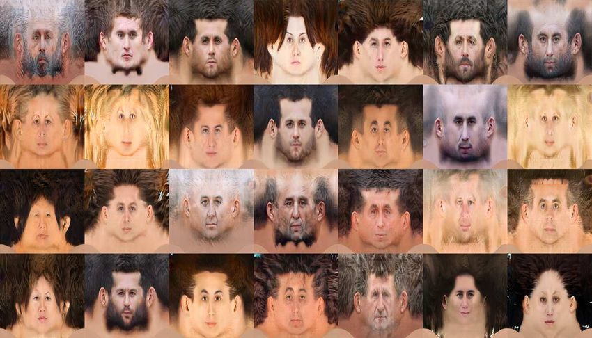
294. Methodology
shows the images generated by the StyleGAN after initial training on CelebA dataset.
Table 4.1: Batch size used for training different resolution layers.
Resolution 4x4 8x8 16x16 32x32 64x64 256x256 512x512
Batch-size 160 140 120 100 80 40 30
Figure 4.4: Generated images after initial training
The next phase of the training is training with the texture dataset with the augmen-
tation and without the augmentations. The evaluation regrading both the trainings is
discussed in the Results and Discussion chapter. The concept of transfer learning is
used in this context. Transfer learning is using an already trained model and retraining
it with a different relatable dataset. As texture and facial images are almost similar,
hence a model trained on facial images can be successfully retrained on textures also.
Transfer learning has several benefits that has made it particularly beneficial in this
scenario:
• A lot of data is usually needed to train the neural network which is not always
available, which is exactly the situation in this case. This is where transfer learning
acts as a saviour because not a lot of data is required for the retraining. With only
860 texture images it was possible to train the entire StyleGAN network, because
it was already trained with the huge CelebA dataset.
• The other advantage is, it provides better results in most cases.
• Last but not the least, it is not needed to train a network every time from scratch,
and hence as a consequence saves a lot of time.
The image below [Figure: 4.5] shows the generated texture of 512x512 resolution, that
was trained with only 860 images of non-augmented textures.
30You can also read