A discontinuous Galerkin finite-element model for fast channelized lava flows v1.0 - GMD
←
→
Page content transcription
If your browser does not render page correctly, please read the page content below
Geosci. Model Dev., 14, 3553–3575, 2021
https://doi.org/10.5194/gmd-14-3553-2021
© Author(s) 2021. This work is distributed under
the Creative Commons Attribution 4.0 License.

A discontinuous Galerkin finite-element model for
fast channelized lava flows v1.0
Colton J. Conroy1,2 and Einat Lev1
1 Lamont-Doherty    Earth Observatory, Columbia University, New York, NY, USA
2 Roy   M. Huffington Department of Earth Sciences, Southern Methodist University, Dallas, TX, USA

Correspondence: Colton J. Conroy (cjc2235@columbia.edu)

Received: 4 June 2020 – Discussion started: 21 September 2020
Revised: 19 February 2021 – Accepted: 6 March 2021 – Published: 11 June 2021

Abstract. Lava flows present a significant natural hazard         were unique in the fact that they produced channelized flows
to communities around volcanoes and are typically slow-           reaching speeds as high as 15 m s−1 (Patrick et al., 2019).
moving (< 1 to 5 cm s−1 ) and laminar. Recent lava flows dur-     These high speeds, coupled with channel geometry (e.g.,
ing the 2018 eruption of Kı̄lauea volcano, Hawai’i, however,      constrictions) produced Reynolds numbers (Re > 3000) that
reached speeds as high as 11 m s−1 and were transitional to       were significantly higher than typical lava flows. To investi-
turbulent. The Kı̄lauea flows formed a complex network of         gate these extreme dynamics we develop a new channelized
braided channels departing from the classic rectangular chan-     lava flow computer model named a discontinuous Galerkin
nel geometry often employed by lava flow models. To inves-        finite-element model for fast channelized lava flows version
tigate these extreme dynamics we develop a new lava flow          1.0.
model that incorporates nonlinear advection and a nonlinear          This paper is organized as follows. In Sect. 1.1–1.3, we
expression for the fluid viscosity. The model makes use of        present the motivation for this work, as well as background
novel discontinuous Galerkin (DG) finite-element methods          on the mathematical tools we employ. In Sect. 2, we present
and resolves complex channel geometry through the use of          the mathematical model and the bottom stress calculation
unstructured triangular meshes. We verify the model against       and detail its nuances. We present the discontinuous Galerkin
an analytic test case and demonstrate convergence rates of        (DG) numerical discretization of the mathematical model in
P + 1/2 for polynomials of degree P. Direct observations          Sect. 3 and verify the model in Sect. 4. In Sect. 5, we evaluate
recorded by unoccupied aerial systems (UASs) during the           the model against observations of lava flows from the 2018
Kı̄lauea eruption provide inlet conditions, constrain input pa-   eruption of Kı̄lauea volcano. We present misfit errors and
rameters, and serve as a benchmark for model evaluation.          root-mean-square errors (RMSEs) for the velocity field from
                                                                  a braided channel section of Fissure 8 and provide quantita-
                                                                  tive insight into physical quantities of the lava flow field in
                                                                  this area, including its thickness and viscosity. We close the
1   Introduction                                                  paper in Sect. 6 with some discussion and conclusions.

On 3 May 2018, Kı̄lauea volcano on the island of Hawai’i          1.1   Motivation
began to erupt from new fissures in the lower East Rift Zone
at the center of the Leilani Estates subdivision. Before ceas-    Typical “operational” lava flow models simulate unconfined
ing in early August 2018, the lava flows destroyed over 650       lava flow in a 2D plan view (e.g., SCIARA, Crisci et al.,
structures and caused significant damage to infrastructure        2004; MAGFLOW, Vicari et al., 2007; LavaPL, Connor
and essential facilities. During the second half of the erup-     et al., 2012; VOLCFLOW, Kelfoun and Vargas, 2015) us-
tion, the flow field established a complex braided channel        ing either cellular automata or depth-averaged equations in
system (which is common to many basaltic flows), originat-        an effort to forecast the area of land inundated by the lava.
ing from fissure number 8 (see Fig. 1). The “Fissure 8” flows     It is often difficult, however, for these models to accurately

Published by Copernicus Publications on behalf of the European Geosciences Union.
3554                                                     C. J. Conroy and E. Lev: Galerkin finite-element model for lava flows

Figure 1. A satellite image (colored, in the background, by DigitalGlobe) overlaid with a thermal aerial orthomosaic (grayscale) where the
white and light gray areas reveal the path of the Fissure 8 flow channel as it was on 21 June 2018. Data and map by USGS. The orange
rectangle depicts the area of UAS site 8 from where the video we analyzed was captured on 22 June 2018. The flat gray areas south of the
active flow channel demarcate the areas inundated by lava during the early stages of the eruption. The top of the image is north. PGV is the
Puna Geothermal Ventures power plant that was heavily impacted by the lava.

reproduce the complicated braided channel network such as               tive lava fields, we now have access to the data required by
those created by Fissure 8. These braided channel networks              sophisticated numerical methods.
are common in natural flows (e.g., Dietterich and Cashman,
2014), and understanding the evolution of the velocity, rheol-          1.2    Shallow-water equations for fast lava flows
ogy, and temperature fields (e.g. in response to pulsating ef-
fusion) within these channels is critical to hazard mitigation          Commensurate with this development in observational capa-
(Patrick et al., 2019). Direct measurements of lava properties          bilities, we introduce a numerical method for modeling fast-
in situ is usually extremely difficult and dangerous. Model-            moving lava flows in complex channels. The high Reynolds
ing lava dynamics within the bounds of an established chan-             number associated with these lava flows, coupled with the
nel can help to better understand material properties of the            fact that the total length of the flows (on the order of kilome-
flowing lava and inform models and decisions.                           ters) is much greater than the flow depth (on the order of me-
   Previous attempts to model channelized lava flows have               ters), means that the dynamics can be well approximated by
made use of simple heuristic formulas such as Jeffreys equa-            two-dimensional depth-integrated equations for mass, mo-
tion for laminar flows (Harris and Rowland, 2015) or Chezy              mentum, and energy. In particular, we utilize a system of dy-
approximations for higher-speed flows (Baloga et al., 1995).            namical equations known as the “shallow water equations”
While convenient, the use of these equations has largely been           (Saint-Venant, 1851), which quantify average horizontal ve-
dictated by the fact that it has been difficult to obtain the           locities and the depth of flow. These equations are tradition-
physical data necessary for advanced modeling efforts (e.g.,            ally used to model free surface flows in coastal oceanic re-
channel domain boundaries, inlet boundary conditions, to-               gions, estuaries, and rivers (Dawson and Mirabito, 2008), al-
pography). However, with the advent of unoccupied aerial                though they have been used to model debris flows (George
systems (UASs, or “drones”) and their ability to survey ac-             and Iverson, 2014) and lava flows (Costa and Macedonio,
                                                                        2005) as well. The main assumption in the shallow water the-

Geosci. Model Dev., 14, 3553–3575, 2021                                                   https://doi.org/10.5194/gmd-14-3553-2021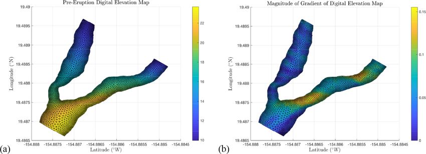
C. J. Conroy and E. Lev: Galerkin finite-element model for lava flows                                                       3555

ory is that the fluid pressure is hydrostatic; gravitational ac-   a large capillary number, which agrees well with the recent
celeration dominates vertical accelerations in the fluid, and      lab experiments of Lev et al. (2020).
the pressure is calculated via the vertical momentum equa-
tion. The formulation of the shallow water equations that          1.3   The discontinuous Galerkin finite-element method
we utilize is designed specifically for advection-dominated
flows (Kubatko et al., 2006), and the pressure gradient term       Because closed-form analytic solutions do not exist to the
is formulated so that the dynamical equations are well bal-        nonlinear shallow water equations and energy equation, we
anced; steady states are preserved, and no artificial motion       construct approximate solutions to these equations using dis-
is induced by numerical artifacts (see Conroy, 2014, for a         continuous Galerkin (DG) finite-element methods (Cockburn
full derivation of the dynamical equations from conservation       and Shu, 2001), which have been used to successfully model
principles).                                                       other geophysical fluid flows including coastal ocean circu-
   Lava flows are distinct from hydrological free surface          lation (Kärnä et al., 2018), hurricanes (Dawson et al., 2011),
flows in the sense that lava transfers heat to its surround-       avalanches (Patra et al., 2006), and debris flows (Conroy and
ings; as lava effuses from a vent it cools along lateral flow      George, 2021). The DG finite-element method differs from
boundaries and can form solid walls (“levees”) that prevent        continuous Galerkin (CG) finite-element methods in that the
the lava from spreading to nearby regions. If lava effusion        DG method solves an integral (or weak) form of the math-
extends for several days, long channels may form that effi-        ematical equations over individual elements and utilizes a
ciently transport lava from the vent to the flow front. The        solution space that is discontinuous across element bound-
speed at which the lava flows through the channel system de-       aries. This allows the DG method to resolve steep gradients
pends on the viscosity of the lava, which in turn is highly de-    that form in the numerical solution, such as the thermody-
pendent on the temperature and chemical composition of the         namic gradients that form at lava channel wall boundaries.
lava (e.g., Griffiths, 2000). The presence of crystals and/or      Even though the DG method is discontinuous it still con-
bubbles in the lava can make its viscosity non-Newtonian           serves mass both locally and globally by utilizing a numer-
(Manga et al., 1998; Mader et al., 2013) and thus strongly         ical flux function (introduced by finite-volume methods; see
dependent on stress gradients and the thermal properties of        LeVeque (2002) for instance) that takes the discontinuous
the lava. To reflect this strong dependence on temperature,        state of physical properties at element boundaries and cre-
we solve a depth-integrated energy equation that quantifies        ates a consistent flow of information from element to element
the thermal evolution of the lava as it interacts with its envi-   (Cockburn and Shu, 2001).
ronment. The depth-integrated energy equation is coupled to           Further, the DG method has been shown to be highly par-
the shallow water equations through a thermally dependent          allelizable using high-performance computing (e.g., Kubatko
nonlinear stress term that reflects the rheology of the lava       et al., 2009, and Patra et al., 2006) and it is amenable to un-
and can account for the presence of crystals and/or bubbles        structured numerical meshes. The latter feature is important
in the lava flow.                                                  when resolving geometrically complex boundaries of a given
   The logistical key to using shallow water equations to          fluid domain, such as the flow fields commonly produced by
model lava flow dynamics rests on the development of the           basaltic flows. For instance, the lava flows that effused from
non-Newtonian bottom stress term. Typical friction drag laws       Fissure 8 formed a complicated network of braided chan-
do not take into account the viscosity of the fluid (due to        nels, with multiple locations of branching and merging. In
the assumption that the fluids inertial acceleration is much       addition, obstructions such as large lava rafts or preexisting
greater than its internal resistance). However, in our partic-     structures caused local disruptions in the flow field, mak-
ular case the flow is not fully turbulent; internal resistance     ing it difficult to evaluate the dynamics using a simplified
needs to be taken into account in some fashion. Thus, we           one-dimensional channelized model, such as those that use a
express the stress at the bottom boundary as a function of         classical rectangular channel geometry (Harris and Rowland,
the temperature and the vertical stress gradient (which is a       2015). To account for these complexities, our new lava flow
function on the vorticity). We solve a thermal boundary layer      model discretizes the lava channel domain with an unstruc-
problem to calculate the temperature at the bottom bound-          tured triangular mesh. This reduces model error as it pertains
ary and utilize the vorticity to determine a virtual length        to a representation of the lava flow domain and is important
scale over which the interior velocity goes from the depth-        when reproducing localized flow features of the lava field,
averaged value to zero. This results in a bottom stress ap-        such as the jet visible in Fig. 4.
proximation that is void of a friction factor (e.g., Manning’s        Model verification consists of solving an analytic test case
n) and allows scientists to study physical properties of the       using forcing functions that we choose to exactly satisfy the
lava that are difficult to measure directly (e.g., viscosity).     equations of motion, and results indicate that for smooth so-
For example, application of the model to the Kı̄lauea 2018         lutions the method converges to the exact solution at a rate of
Fissure 8 lava flows reveals that the lava behaved as a shear      P + 1/2 for polynomials of degree P.
thickening fluid due to the high bubble content (≈ 50 %) with

https://doi.org/10.5194/gmd-14-3553-2021                                             Geosci. Model Dev., 14, 3553–3575, 2021
3556 C. J. Conroy and E. Lev: Galerkin finite-element model for lava flows
2 Mathematical model – Outlet boundary condition:
zero change in normal velocity, ∂u/∂ n̂ = 0;
Fluid flow on sloped terrain can be quantified in a Carte- zero change in pressure, ∂p/∂ n̂ = 0;
sian coordinate (x, y, z) system over a time-dependent do- zero change in heat content, ρcp ∂T /∂ n̂ = 0.
main (t) ∈ R3 by solving Eulerian conservation equations
of mass, linear momentum, and energy, – Free surface boundary condition at z = ζ :
∂ρ no relative normal flow,
+ ∇ · (ρu) = 0, (1) ∂ζ /∂t = −u(∂ζ /∂x) − v∂(ζ /∂y) + w;
∂t
∂ 0 atmospheric pressure, p = patm ;
(ρu) + ρu · ∇u + ∇p − ∇ 0 τ = f b , (2) surface shear stress, τsx = −τxx (∂ζ /∂x)−τyx (∂ζ /∂y)+
∂t
∂T τzx , τsy = −τxy (∂ζ /∂x) − τyy (∂ζ /∂y) + τzy ;
ρcp + ρcp (u · ∇T ) − ∇ · q = q̇. (3) heat loss via radiation and
convection, 4
∂t
q · n̂ = σB T 4 − Tatm
4 + kc (T − Tatm ) 3 .
0
In Eqs. (1)–(3), ρ is the fluid
density, 0 u = (u, v, w) is the
∂ ∂ ∂ – Bottom boundary condition at z = −h:
fluid velocity vector, ∇ = ∂x , ∂y , ∂z is the gradient oper-
ator, p is the pressure, and τ is the stress term, no slip velocity, u = 0;
bottom shear stress, τbx = τxx (∂h/∂x) + τyx (∂h/∂y) +
τxx τxy τxz τzx , τby = τxy (∂h/∂x) + τyy (∂h/∂y) + τzy ;
τ = τyx τyy τyz . (4)
heat loss via conduction, q · n̂ = (kb /hb ) T − Tground .
τzx τzy τzz
In the boundary conditions above, n̂ is the unit normal
We denote the x component of gravitational acceleration that
vector to the wall boundary, outlet boundary, inlet boundary,
is tangential to the sloped surface by gx ; gy is the y com-
moving free surface, and bottom boundary, respectively; t̂ is
ponent of gravitational acceleration that is tangential to the
the unit tangential vector to the wall; τ wall is the tangential
sloped surface, and gz is gravitational acceleration that is nor-
shear stress at the wall; and σ wall is the normal stress at the
mal to the sloped surface. Collectively, these terms form the
wall. We denote the temperature at the wall by Tw , kw is the
body force vector f b = (gx , gy , gz )0 acting on the fluid. T
thermal conductivity of the wall, and hw is the thickness of
is the temperature of the fluid, cp is the specific heat capac-
0 the thermal boundary layer through which heat is conducted
ity of the fluid, q = kT ∂T∂x , k T
∂T
∂y , k T
∂T
∂z is the heat flux from the lava flow to the wall. We measure the free surface,
through the fluid (kT is a conduction heat transfer coefficient ζ , relative to a steady depth of flow, h(x, y), that serves as
that measures the spread of heat within the fluid), and q̇ quan- the zero datum in the z direction (see Fig. 2). The surface
tifies the generation and dissipation of heat within the fluid. forces acting on the free surface consist of the atmospheric
Equations (1) and (2), taken together, are the Navier– pressure, patm , along with a surface shear stress applied by
Stokes equations and quantify the force dynamics acting on the wind τ s = (τsx , τsy )0 . Heat transfer from the lava surface
the fluid (see Conroy, 2014, for a derivation from first prin- to the surrounding atmosphere is dominantly due to radia-
ciples). Equation (3) is the thermal energy equation: it quan- tion and air convection, where is the emissivity of the lava,
tifies the transport of energy through the fluid due to inter- σB is the Stefan–Boltzmann constant, Tatm is the temperature
nal temperature gradients and differences between the fluid of the surrounding atmosphere, and kc is the convection heat
temperature and the temperature of the surrounding medium transfer coefficient. The main resisting force in dense shal-
(see Moran et al., 2003, for instance). To apply Eqs. (1)–(4) low mass high-speed flows comes from the bottom stress,
to channelized lava flow we need to supplement them with τ b = (τbx , τby )0 , which is a function of the temperature of the
appropriate boundary conditions and define the stress matrix lava at the basal boundary, where Tground is the temperature
τ . Here, we assume that the system of equations given by of the ground and hb is the depth of the thermal boundary
Eqs. (1)–(3) are subject to the following kinematic, dynamic, layer through which heat is transferred from the lava to the
and thermal boundary conditions: ground.
Theoretically, we could define τ and solve Eqs. (1)–(3)
– Channel wall boundary condition:
along with the prescribed boundary conditions to model
no normal flow u · n̂ = 0;
channelized lava flows. In practice, however, we need to sim-
no pressure gradient, ∂p/∂ n̂ = 0;
plify Eqs. (1)–(3) to make the solution more tractable. More
slip velocity, u · t̂ = f (τ wall , σ wall );
specifically, we assume the following: (i) the lava flow field
heat loss via conduction, q · n̂ = (kT /hw ) (T − Twall ).
is incompressible, (ii) vertical accelerations in the lava are
– Inlet boundary condition: dominated by gravity, (iii) lava flow lengths are much greater
prescribed velocity, u · n̂ = prescribed; than the flow depth, and (iv) horizontal flow speeds are large
prescribed pressure, p = prescribed; enough that stress gradients are dominated by the first two
prescribed heat content, ρcp T = prescribed. columns of the stress matrix τ .
Geosci. Model Dev., 14, 3553–3575, 2021 https://doi.org/10.5194/gmd-14-3553-2021
C. J. Conroy and E. Lev: Galerkin finite-element model for lava flows                                                                      3557

Figure 2. A vertical cross section along the center line of the flow, showing the coordinates (x and z, with y the across-flow direction) and the
heat transfer mechanisms considered in the model (conduction to the base, advection by the flow, and heat loss by radiation and convection
at the surface).

   Assumption (i) reduces the conservation of mass equation
to ∇ · u = 0, while assumptions (ii) and (iv) reduce the z-
                                                                           ∂H     ∂          ∂
momentum equation to                                                           +    (H u) +    (H v) = 0,                                    (6)
                                                                            ∂t   ∂x         ∂y
∂p
   = ρgz ,                                                                 ∂H u     ∂  2 ∂                 ∂
∂z                                                                               +     Hu +      (H uv) + H    (gz ζ ) + H gx =
                                                                            ∂t     ∂x         ∂y            ∂x
which we can leverage to determine the pressure. Integrating               1
from the free surface ζ down to a given z coordinate yields                   τs − τbx + fx ,                                                (7)
                                                                           ρ x
p = patm + ρgz (ζ − z) .                                          (5)      ∂H v    ∂            ∂  2    ∂
                                                                                +     (H uv) +     Hv +H    (gz ζ ) + H gy =
                                                                            ∂t    ∂x           ∂y        ∂y
  We assume that gradients in patm are negligible and the
horizontal pressure gradient in Eq. (2) becomes                            1
                                                                              τs − τbx + fy ,                                                (8)
                                                                           ρ y
∇p = ∇(ρgz ζ ),
                                                                           ∂H T    ∂      ∂

                ∂    ∂
                       0                                                       +    H uT +    H vT = qs + qb + ∇ · q i + q̇,                (9)
where ∇ = ∂x      , ∂y    . We further simplify the mathematical            ∂t    ∂x        ∂y
model and eliminate the vertical dimension by integrating ∇ ·              where fx and fy are the x component and y component of the
u = 0 and Eqs. (2) and (3) over the depth of the lava flow                 depth-averaged gradient of the shear stresses acting on verti-
(from −h to ζ ). We then apply Leibniz’s integral rule, utilize            cal fluid planes, qs is the heat flux through the free surface,
the free-surface and bottom boundary conditions, assume the                qb is the heat flux at the bottom boundary, ∇ · q i quantifies
density is constant, and simplify the resulting expression to              depth-averaged internal conduction, and q̇ represents depth-
arrive at the following depth-integrated equations:                        averaged internal heat generation and dissipation. The depth-
                                                                           averaged velocity, u = (u, v), and depth-averaged tempera-
                                                                           ture, T , are defined as

https://doi.org/10.5194/gmd-14-3553-2021                                                       Geosci. Model Dev., 14, 3553–3575, 2021
3558                                                     C. J. Conroy and E. Lev: Galerkin finite-element model for lava flows

           Zζ                                                         ∂ζ    ∂          ∂
   1                                                                     +    (H u) +    (H v) = 0,                                (13)
u=              u dz,                                         (10)    ∂t   ∂x         ∂y
   H
           −h
                                                                      ∂H u    ∂  2      ∂
           Zζ                                                              +     H u + P + (H uv) + H gx
       1                                                               ∂t    ∂x           ∂y
v=              v dz,                                         (11)           ∂h τbx
       H                                                                = gζ    −    ,                                             (14)
           −h                                                                ∂x    ρ
           Zζ
    1                                                                 ∂H v    ∂            ∂  2
T =             T dz.                                         (12)         +    (H uv) +      H v + P + H gy
    H                                                                  ∂t    ∂x           ∂y
        −h
                                                                             ∂h    τ by
                                                                        = gζ    −       ,                                          (15)
The above system of depth-integrated equations (Eqs. 6–9)                    ∂y     ρ
can be further simplified due to the dynamics of high-speed
flows. More specifically, fx and fy are negligible in high-           ∂H T       ∂          ∂
speed flows except at no-slip and small-slip velocity bound-                 +        H uT +        H vT = qs + qb ,                (16)
                                                                        ∂t      ∂x             ∂y
ary conditions where large stress gradients form due to the
                                                                      where P = 21 gz H 2 − h2 is the pressure flux and ∂h/∂x

decay of the velocity field to a value of zero (or near zero).
In our quantitative analysis of UAS footage from the 2018             and ∂h/∂y quantify the gradient in the steady reference depth
Kı̄lauea eruption, lava flow velocities at channel wall bound-        of flow that ζ is measured relative to. We supplement the sys-
aries were much greater than zero, and therefore we utilize a         tem of equations given by Eqs. (13)–(16) with initial condi-
slip (no-flow) channel wall boundary condition and neglect            tions along with the channel wall, inlet, and outlet boundary
fx and fy in this initial version of the model (see Rao and           conditions. It can be noted that the depth-integrated mass and
Rajagopai, 1999, for an in depth investigation on channel             momentum equations given by Eqs. (13)–(15) are well stud-
wall boundary conditions in terms of the slip versus no-slip          ied in the literature and are commonly used to model shallow
condition). The surface stress terms (τx , τy )0 in the depth-        mass flows such as coastal ocean circulation and hurricane
integrated equations account for wind stress on the lava flow,        storm surge; see, for example, Dawson et al. (2011) and Ku-
which we assume to be negligible due to the ratio of the              batko et al. (2006). The addition of the energy equation com-
density of air to the density of lava being much less than            plicates the solution of Eqs. (14) and (15) due to the fact that
one. We include the effect of heat conduction at the chan-            the bottom stress term, τ b = (τbx , τby )0 , is now a function of
nel wall boundaries, but we neglect heat conduction in the            both nonlinear velocity gradients and temperature.
interior of the lava due to the high speed of the flow, and
we set ∇ · q i = 0. Internal heat generation and dissipation          2.1   Quantifying the bottom stress term
can be significant in lava flows with a high crystal content
(Griffiths, 2000) and in lava flows in closed tubes (Costa and        In the equations of motion (Eqs. 14 and 15), we define the
Macedonio, 2005). The Fissure 8 lava flows were hot with              bottom stress term using a Herschel–Bulkley model (Her-
limited crust cover, and samples indicate that the crystal con-       schel and Bulkley, 1926),
tent was low in the channel section that we apply the model
                                                                                     ∂u               ∂u
to (Gansecki et al., 2019), and therefore we neglect q̇ in the        τ b = τ zx = µ    + τyield sgn       ,                (17)
current model but plan to include it in future releases.                             ∂z               ∂z
   It can be noted that the pressure     0      gradient terms,      where τ b = τ zx = (τzx , τzy )0 , τyield is the yield strength of
                  ∂             ∂
(1/ρ)∇p = H ∂x      (gz ζ ), H ∂x (gz ζ ) , in Eqs. (7) and (8) are   the fluid, sgn denotes the sign of the argument, and µ is the
non-conservative product terms that can lead to entropy-              nonlinear viscosity, defined as
violating numerical fluxes if care is not taken in evaluating
them numerically (see LeVeque, 2002, for instance). To cir-                        n−1
                                                                              ∂u
cumvent this issue, we make use of the fact H (x, y, t) =             µ=K                .                                         (18)
                                                                              ∂z
ζ (x, y, t) + h(x, y) and rewrite Eqs. (7) and (8) in the con-
servative form (Kubatko et al., 2006),                                The symbol K in Eq. (18) represents the consistency of the
                                                                      lava and can be modeled solely as a function of temperature,
                                                                      while the power law exponent, n, is typically a function of the
                                                                      particle content (crystals and/or bubbles) of the lava (which
                                                                      in turn can be a function of temperature); see Castruccio et al.
                                                                      (2010) and Castruccio et al. (2014) for example. We quantify
                                                                      the temperature dependency of the lava consistency (K) in

Geosci. Model Dev., 14, 3553–3575, 2021                                                  https://doi.org/10.5194/gmd-14-3553-2021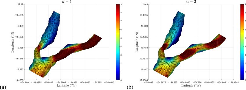
C. J. Conroy and E. Lev: Galerkin finite-element model for lava flows 3559
a fashion similar to Sonder et al. (2006) and use the Vogel– It can be noted that in the expression above, δ z = (δzx , δzy )0 ,
Fulcher–Tammann (VFT) silicate melt model of Giordano is a measure of a virtual length over which the shear stress is
et al. (2008), applied. We determine δ z by taking into account the vorticity
of the lava flow field, which is defined as
K B
log = A+ , (19)
K0
T (K) − C ∂w ∂v ∂w ∂u ˆ ∂u ∂v
ω= − î + − j+ − k̂, (22)
where A is the value of log K/K0 at infinite temperature, K0 ∂y ∂z ∂x ∂z ∂y ∂x
is a constant set to 1 sn−1 , and B and C are parameters that
depend on the composition of the lava. The model assumes where î, jˆ, and k̂ are unit vectors in the x, y, and z di-
that A is a constant for all silicate melts regardless of com- rections, respectively. We solve an auxiliary problem over
position, and thus it represents the high temperature limit for a pseudo-depth of the lava that consists of an upper mixed
silicate melt viscosity. Once the parameter A is fixed then the layer where u(x, y, z) ≡ u(x, y) and a lower layer where
parameters B and C are determined via a linear ensemble of (∂u/∂z, ∂v/∂z)0
(∂w/∂x, ∂w/∂y)0 . We assume that the
combinations of oxide components and a subordinate num- vorticity in the upper layer is equal to the vorticity in the
ber of multiplicative oxide cross terms; see Giordano et al. bottom layer (in terms of magnitude) at the coordinate point
(2008) for the full details of the model. where ∂u/∂z 6 = 0 (i.e., at the interface between the two lay-
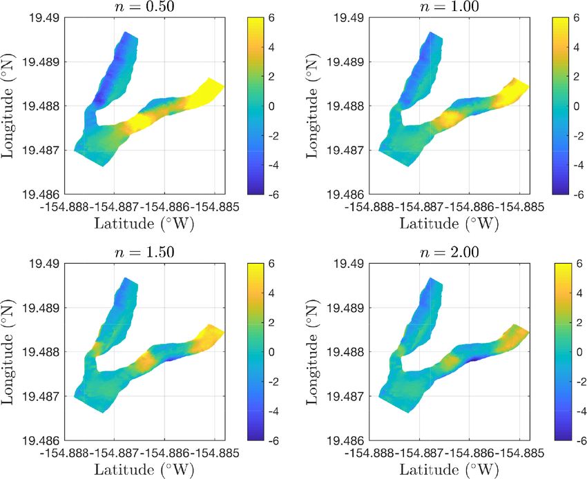
The power law exponent of the viscosity term quantifies ers). This allows us to calculate the vorticity in the upper
the effect that stress gradients have on the material proper- layer and then use this value to determine δ z . In other words,
ties of the fluid. A value of n = 1 corresponds to a Newtonian we answer the following question: given a measure of the
fluid, while n < 1 or n > 1 corresponds to a non-Newtonian vorticity associated with the depth-averaged velocity field,
fluid. If n > 1 then the fluid viscosity increases with increas- what is the associated length scale over which the depth-
ing shear rate (shear thickening), while if n < 1 the fluid vis- averaged velocity must decay to a value of zero (the bottom
cosity decreases with increasing shear rate (known as shear boundary condition) to ensure that the internal vorticity of
thinning). Typically, if the lava is sufficiently hot and de- the flow is conserved? It can be noted that an implicit as-
gassed, then the lava stress can be modeled with a Newtonian sumption in depth-integrated models is that internal friction
approximation and n = 1. However, if bubbles and/or crys- in the vertical is null compared to the friction at flow bound-
tals are present in the lava (depending on the lava source and aries. This, along with assumption (i) and a constant density,
the amount of degassing that has occurred), then these struc- implies conservation of vorticity about the î and jˆ directions
tures will deform and realign under an applied shear stress. except at flow boundaries). The key to this approach relies
This consequently causes the viscosity of the lava to become on calculating a measure for the vertical velocity in the up-
thinner in some situations and thicker in others depending on per layer, which we achieve by making use of the kinematic
how the structures rearrange. Lava flows with a high crystal boundary condition,
content are typically pseudo-plastic and shear thinning; the ∂ζ ∂ζ ∂ζ
crystal structure of the lava resists the flow of the lava and the +u +v = w|z = ζ , (23)
∂t ∂x z=ζ ∂y z=ζ
lava will not flow unless a yield strength is surpassed. In this
case, the lava will continue to flow more readily as the shear coupled with the depth-integrated continuity Eq. (13) to ob-
stress increases. The opposite tends to occur when a lava flow tain a measure of the vertical velocity w. More specifically,
has a high bubble content at higher capillary numbers; large expanding derivatives in Eq. (13), solving for ∂ζ /∂t, while
stress gradients in the flow cause the bubbles to rearrange in substituting this result into Eq. (23) and noting that in the
a fashion that increases the viscosity and the lava behaves as upper layer (u, v, w) ≡ (u(ζ ), v(ζ ), w(ζ )) yields
a shear thickening fluid.
The bottom stress term is a function of the velocity gradi- ∂u ∂v
w=ζ +ζ . (24)
ent evaluated at the bottom boundary, which we do not have ∂x ∂y
access to in the depth-averaged equations, and therefore we
define the bottom stress in terms of the depth-averaged ve- The relevant vorticity terms in Eq. (22) include the î and jˆ
locity as components. By definition, ∂u/∂z = ∂v/∂z = 0 over the up-
per layer so that the vorticity component about the x axis
u u
τbx ≡ µ + τyield sgn is ∂w/∂y and the vorticity component about the y axis is
δz δz ∂w/∂x. Because the bottom boundary condition is modeled
∂u ∂u as a rigid wall where u = 0 and the fluid is incompressible, a
≈µ + τyield sgn , (20)
∂z ∂z vorticity layer forms in the fluid near the solid boundary that
resists the local rotation of the fluid (this is the reason why
where
the rigid boundary does not deform). The vorticity created at
n−1
u the boundary resists the rotation of the interior and is equal
µ=K . (21) to ∂v/∂z about the x axis and ∂u/∂z about the y axis (see
δz
https://doi.org/10.5194/gmd-14-3553-2021 Geosci. Model Dev., 14, 3553–3575, 20213560 C. J. Conroy and E. Lev: Galerkin finite-element model for lava flows
Schlichting et al., 1968). Now, if we assume that each vor- where kc is a heat transfer coefficient (e.g., Patrick et al.,
ticity component over the bulk of the flow is equal to each 2004). We quantify heat transfer from the lava to the ground
vorticity component in the boundary layer at the coordinate via conduction (Patrick et al., 2004),
point where (∂u/∂z, ∂v/∂z)0 is no longer equal to zero, then
the virtual length over which the shear stress is applied is qb = kb T − Tground , (29)
given by
where Tground = f (x) is the temperature of the ground in
u v contact with the lava flow field and kb measures the thermal
δzx = and δzy = . (25)
∂w/∂x ∂w/∂y conductivity of the ground. We utilize Eq. (29) to determine
the temperature near the bottom boundary of lava flow field
It can be noted that as (∂w/∂x, ∂w/∂y) goes to 0, the ver-
which we use to evaluate the nonlinear viscosity in the bot-
tical stress in the fluid goes to 0. We can rewrite expression
tom stress term in the equations of motion. More specifically,
(Eq. 25) solely in terms of the depth-averaged variables using
we can rewrite Eq. (29) in terms of a depth-dependent ther-
Eq. (24):
mal boundary layer temperature, T (z),
∂v −1
∂ ∂u
δz x = u ζ +ζ and ∂T k̃b
∂x ∂x ∂y = T − Tground , (30)
∂z hb
∂v −1
∂ ∂u
δzy = v ζ +ζ . (26)
∂y ∂x ∂y where k̃b is the thermal boundary layer conductivity con-
stant and hb (x, y) is the thickness of the thermal bound-
It can be noted that even though we do not explicitly include ary layer (see Fig. 2). We solve Eq. (30) over the thermal
horizontal shear stresses in the Kı̄lauea simulations presented boundary layer defined in the z direction from z = zb (x, y)
in Sect. 5 (due to the high Re number), the virtual length used to z = −h(x, y) by setting zb (x, y) to a relative zero. We
to quantify the bottom stress as defined in Eq. (26) is a func- then integrate Eq. (30) over a thermal boundary coordinate
tion of horizontal shear within the fluid. Further, we wish defined from z̃ = 0 to z̃ = −hb (x, y). It can be noted that the
to emphasize that the virtual length, δ z , is non-physical and relationship between z̃ and z is given by z̃ = z − zb so that
is not necessarily less than the lava flow thickness (H ); it hb = h − zb . Equation (30) is a non-homogeneous, constant
merely is a measure to ensure that (u − 0)/δ z ≈ ∂u/∂z at the coefficient ordinary differential equation that has the follow-
bottom boundary in a fashion that conserves internal vortic- ing solution:
ity, i.e., it ensures that the interior of the flow field is irrota-
tional about the î and jˆ coordinate axis.
!
k̃b
T (z̃) = Tint − Tground exp z̃ + Tground , (31)
2.2 Heat transfer hb
As soon as lava effuses from an active vent it begins to de- which gives an expression for the temperature profile over the
gas and transfer heat to its surroundings. Lava cools through thermal boundary layer of the lava (z̃ ∈ [0, −hb ]). Evaluating
the mechanisms of radiation, conduction, and convection in Eq. (31) at z̃ = −hb and setting the interior temperature (Tint )
the air above it (we neglect heating from viscous dissipation, to the depth-integrated value (T ), we have
which is small compared to heat loss through radiation and
conduction for the low-viscosity flows we are considering
T = T − Tground exp −k̃b + Tground . (32)
here, e.g., Harris and Rowland, 2001). We quantify heat loss z̃ = −hb
due to radiation via Stefan’s law (Griffiths, 2000),
We use this temperature to evaluate the consistency in the
σB 4 4
bottom stress approximation,
qs = T − Tatm , (27)
ρcp
where is the emissivity of the lava, σB is the Stefan– K =K T . (33)
z = −h z̃ = −hb
Boltzmann constant, and Tatm is the temperature of the sur-
rounding atmosphere in degrees Kelvin. When lava tempera- The greater the thermal conductivity of the boundary layer,
tures fall below the solidus (e.g., ∼ 950 C for Kı̄lauea lavas), the closer the boundary temperature is to the ground temper-
buoyancy-driven convection in the air above the lava be- ature; however, in general, there is usually a steep gradient in
comes the dominant mode of heat transfer at the lava surface the temperature at the interface between the boundary of the
instead of radiation (due to crust formation) (Griffiths, 2000). flowing lava and the ground that the lava is conducting heat
In this case we set qs in the energy equation to to. It can be noted that we also use an analogous approach to
4/3 calculate the temperature of the lava at channel wall bound-
qs = kc T − Tatm , (28) aries.
Geosci. Model Dev., 14, 3553–3575, 2021 https://doi.org/10.5194/gmd-14-3553-2021C. J. Conroy and E. Lev: Galerkin finite-element model for lava flows 3561
2.3 Steady reference depth of flow h automatic mesh generator known as ADMESH+ (Conroy
et al., 2012). ADMESH+ solves a number of differential
We have two options to calculate the steady reference depth equations to calculate a mesh size function that determines
of flow (h) of the lava that we use as a zero datum to measure local element sizes based on the curvature of the boundary,
the free surface from. Our particular choice depends on the channel width, and changes in the topography and domain
inflow data available to the model. For instance, if a full set slope to create a high-quality unstructured simplex mesh (the
of temporally varying inflow data is available, we set h equal elements are close to equilateral triangles). The only input re-
to the time average thickness associated with the data, i.e., quired by the program is a list of points defining the boundary
Ztf and the topography of the domain.
1 Qin · n̂
h= uin · n̂ dt, (34) 3.2 A weak form and the semi-discrete equations
(tf − ti ) win
ti
Given the finite-element partition, Th , of the domain , we
where Qin · n̂ is the inflow flux normal to the boundary and
obtain a weak form of Eq. (35) if we first multiply Eq. (35)
win is the width of the inflow boundary normal to the flow.
by a sufficiently smooth test function ψ(x, y) ∈ V, integrate
If, however, the only inflow data available to the model is a
over each element j ∈ Th , and then integrate the flux term
set of time-averaged data, then we set h to the solution of
by parts,
the steady, linear system of equations associated with the full
nonlinear system of equations given by Eqs. (13)–(16). Z
∂U (i)
Z Z
ψdA − F(i) · ∇ψdA + F(i) · n̂ ψdS =
∂t
j j ∂j
3 Numerical discretization Z
S (i) ψdA, U (i) , ψ ∈ V , (36)
To develop our numerical methods, we rewrite the system of
j
Eqs. (1) in the compact form,
∂U (i) for i = 1, 2, 3, 4 and j = 1, . . ., N , where N is the total num-
+ ∇ · F(i) (U ) = S (i) (U ), i = 1, 2, 3, 4, (35) ber of elements of the triangulation Th . In the equation above,
∂t
n̂ is the outward unit normal to the element boundary ∂j .
where U (i) , F(i) , and S (i) are the i-th row entries of the vec- Rather than seek solutions to Eq. (36), we search for solu-
tors U , S, and the flux function matrix F, defined as tions in the finite dimensional subspace of functions defined
H
as
Hu
U = Vhp = ψ : ψ j ∈ P` j , ∀j , (37)
Hv ,
HT where P` demarcates the space of polynomials of at most
H u, Hv
degree ` that is not necessarily continuous across element
H u2 + P , H uv boundaries. In other words, given a set of basis functions φ =
(i)
F= H uv, H v2 + P
, (φ0 , φ1 , . . ., φ` )0 , we express the trial solution (Uh ∈ Vhp )
H uT , H vT and test function (ψh ∈ Vhp ) as
0 (i)
X̀ (i)
−g H + gζ ∂h − τbx Uh = Ul (t)φl (x), (38)
x ∂x ρ j
S= τby ,
l=0
−gy H + gζ ∂h ∂y − ρ
qs + qb and
where P = 12 gz H 2 − h2 .
X̀
ψh = ψl (t)φl (x), (39)
j
l=0
3.1 Finite-element partition
(i) 0
(i) (i)
To apply a DG spatial discretization to our mathematical where U0 , U1 , . . ., U` are the time-dependent degrees
model (Eq. 35) over a lava flow channel (see Fig. 5, for of freedom of the finite-element solution and i = 1, 2, 3, 4.
example), we begin by introducing a partition of the two- We use products of Jacobi polynomials of degree `, {Pl }`l=0 ,
dimensional domain . The complexities of the domain as the basis for Vhp . The orthogonal triangular basis is de-
boundary, ∂, are such that an unstructured finite-element fined in terms of a “collapsed coordinate” system that results
partition (or mesh) is necessary to properly capture its intri- in a matrix-free implementation of the method; see Kubatko
(i)
cacies. More specifically, we obtain unstructured triangula- et al. (2006) for more details. Substituting Uh and ψh into
tions (that we denote by Th ) of the channel domain via an Eq. (36), we arrive at the discrete weak form of the problem:
https://doi.org/10.5194/gmd-14-3553-2021 Geosci. Model Dev., 14, 3553–3575, 20213562 C. J. Conroy and E. Lev: Galerkin finite-element model for lava flows
∂Fi
where the Jacobian matrices Jij = ∂xj are
0 1 0 0
gz H − u2
2u 0 0
Jx =
,
−uv v u 0
−uT T 0 u
Figure 3. Jump in numerical solution U h at an element edge ∂j .
and
0 0 1 0
(i)
find Uh ∈ Vhp such that for all test functions ψh ∈ Vhp for
i = 1, 2, 3, 4, the expression,
−uv v u 0
Jy = .
gz H − v 2
Z
∂Uh
(i) Z Z 0 2v 0
F(i) (U h ) · ∇ψh dA + F̂(i) · n̂ ψh dS
ψh dA −
∂t
j j ∂j −vT 0 T v
Z
= S (i) (U h )ψh dA, (40) The so-called “normal Jacobian matrix” is then defined by
j
Jn = Jx nx + Jy ny , (43)
holds over each element j ∈ Th , where S (i) (U h ) is the where nx and ny are the x and y components of the normal
source term evaluated in Vhp and F̂(i) is a suitably chosen edge vector n̂. In general, if J is a square (m × m) matrix
numerical flux. with m real eigenvalues, then it can be decomposed into its
eigensystem,
3.2.1 Numerical flux
Jx = R(x) 3(x) R−1 −1
(x) , and Jy = R(y) 3(y) R(y) , (44)
The space of functions defined by Eq. (37) is not necessar- where R(·) is the matrix of right eigenvectors, 3(·) is the di-
ily continuous across element boundaries, and thus can be agonal matrix of eigenvalues, and R−1 (·) is the matrix of left
dual-valued (see Fig. 3, for example). To remedy this incon- eigenvectors (LeVeque, 2002). To determine 3(x) and 3(y)
sistency, we replace the dual-valued flux in Eq. (36) with a
we solve for the roots of det J(·) − λI = 0, which gives the
so-called numerical flux (F̂) that makes use of the left and following eigenvalues,
right limits of the trial solution to produce a single-valued
flux across a given element’s boundary. λ1,2 = unx + vny ,
More specifically, given an arbitrary function wh ∈ Vhp at p p
an element boundary point xi , we set the left and right limits λ3 = u + gz H nx + v + gz H ny ,
of the function to wh− ≡ wh (x− + +
i ) and wh ≡ wh (xi ), respec-
p p
λ4 = u − gz H nx + v − gz H ny . (45)
tively. In this work we utilize the local Lax–Friedrichs (LLF)
flux, which defines the numerical flux operator as (·)
Each eigenvector (r i ) can be determined by solving (J(·) −
λi I)r i = 0, wherehI is the identity imatrix, 0 is a vector of
F(i) · n̂
b (·) (·) (·) (·)
zeros, and R(·) = r 1 , r 2 , r 3 , r 4 . Solving for the eigen-
1 (i,+) 1
(i,+) (i,−)
= F + F(i,−) · n̂ − |λmax | Uh − Uh , vectors we have
2 2
for i = 1, 2, 3, 4, (41)
0 0 1/T 1/T
√ √
R(x) = 0 0 (u + gz H )/T (u − gz H )/T ,
1 0 v/T v/T
where λmax is the maximum eigenvalue of the normal (to the 0 1 1 1
element edges) Jacobian matrix. When solutions to Eq. (35)
are sufficiently smooth, we can rewrite Eq. (35) in the quasi- and
linear form,
0 0 1/T 1/T
1 0 u/T u/T
R(y) = √ √ .
∂U 0 0 (v + gz H )/T (v − gz H )/T
+ Jx (U )x + Jy (U )y = S, (42) 0 1 1 1
∂t
Geosci. Model Dev., 14, 3553–3575, 2021 https://doi.org/10.5194/gmd-14-3553-2021C. J. Conroy and E. Lev: Galerkin finite-element model for lava flows 3563
We use the full eigensystem in the slope-limiting process that where Lhp is the DG spatial operator. We evaluate the in-
stabilizes the method for polynomials of degree greater than tegrals in Eq. (47) using numerical integration rules of suf-
or equal to one (Cockburn and Shu, 2001), and we set λmax ficiently high degree (Kubatko et al., 2006) and discretize
in the LLF flux to the maximum value of (λ1 , λ2 , λ3 , λ4 ). Eq. (48) with so-called strong stability-preserving (SSP)
It can be noted that to mathematically close the solution Runge–Kutta (RK) methods (Kubatko et al., 2014). The un-
method of the discrete DG system of equations we need to known polynomial basis coefficients that define the solution
numerically evaluate expression (Eq. 26) to determine δ z . over a given element, j , are advanced in time from tm to
More specifically, we discretize Eq. (26) using a local discon- tm+1 via
tinuous Galerkin (LDG) method (Cockburn and Chi-Wang, (i) (i)
1998) analogous to the method used in Conroy and Kubatko 1. Set Ũ 0 ← Ũ m , for i = 1, 2, 3, 4.
(2016) to evaluate second-order derivative terms (see Con-
roy, 2014, for a detailed discussion on application of the 2. For each stage r = 1, 2, . . ., S, set
LDG method to shallow mass geophysical fluid flows). r
!
X
Ũ (i)
r ← 5h αrs wrs ,
3.3 Strong stability-preserving Runge–Kutta time
s=1
discretizations
rs (i) βrs
w = Ũ s−1 + 1t Lh Ũ s−1 , tm + δs 1t .
Application of the DG spatial operator to Eq. (40) results in αrs
a system of ordinary differential equations (ODEs) for each
element, (i)
3. Finally, set Ũ m+1 ← Ũ S .
(i)
(i)
(i)
dŨ j (i) It can be noted that 5h is a slope limiter that dampens
M̃j = bj , i = 1, 2, 3, 4 and j = 1, . . ., N ,
dt overshoots and undershoots at solution discontinuities when
(46) polynomial approximations greater than 0 are used for the
(i) basis (Cockburn and Shu, 2001), S is the number of stages
where N is the number of elements in Th , Ũ j = of the RK method, δs 1t is a sub-time step of the time step
(i) 0
(i) (i) 1t, and the αrs and βrs are coefficients that define the RK
Uj,0 , Uj,1 , . . ., Uj,` are vectors of the degrees of free-
(i) method. In particular, αrs and βrs conform to the following
dom (i.e., the polynomial basis coefficients), and bj = constraints:
(i) 0
(i) (i)
R j,0 , R j,1 , . . ., R j,` with,
1. αrs = 0 if and only if βrs = 0;
Z Z
(i) (i) (i)
R j,l = Fj · ∇φl dA − F̂j · n φl dS 2. αrs ≥ 0 and βrs ≥ 0;
j ∂j Pr
Z 3. s=1 αrs = 1.
(i)
+ Sj φl dA. (47)
Because we use explicit RK methods, the time step of the
j model is limited by a CFL condition; see Kubatko et al.
(i) (2014) for more details.
M̃j is the mass matrix,
R
φ1 φ1 dA 0 ... 0
j 4 Verification
R ..
Verification of the DG solution of the mass and momentum
0 φ2 φ2 dA 0 .
(i) j equations in the depth-averaged and full three-dimensional
M̃j = ,
case is well documented and can be found in Conroy and
.. .. Kubatko (2016), Dawson and Aizinger (2005), and Ku-
. 0 . 0
R batko et al. (2006). To verify our DG solution method for
0 0 φ` φ` dA
... the fully coupled mass, momentum, and energy (depth-
j
averaged) equations, we solve a test problem that is designed
which is diagonal due to the choice of basis. Left multiplying to model a free surface wave propagating through a lava
(Eq. 46) by the inverse of the mass matrix, we have channel using the method of manufactured solutions (see
Griffiths, 2000, for a discussion on free surface waves in lava
dŨ (i) (i) −1 (i) channels at high Re number and Le Moigne et al. (2020) for
= M̃j bj = Lhp (Ũ ),
dt a detailed investigation on standing waves in lava flow chan-
with i = 1, 2, 3, 4, and j = 1, . . ., N , (48) nels). We choose u, v, and H so that the depth-averaged mass
https://doi.org/10.5194/gmd-14-3553-2021 Geosci. Model Dev., 14, 3553–3575, 20213564 C. J. Conroy and E. Lev: Galerkin finite-element model for lava flows
Table 1. L2 errors using P0 for (ζh , uh , v h , T h ).
Mesh ||ζh − ζ ||2 Order ||uh − u||2 Order ||v h − v||2 Order ||T h − T ||2 Order
dx0 3.91 – 8.81 – 9.24 – 2126.3 –
dx1 2.06 0.92 4.48 0.98 4.82 0.94 1227.7 0.79
dx2 1.39 0.97 3.01 0.98 3.30 0.93 875.11 0.84
dx3 0.31 1.08 0.77 0.98 0.77 1.05 218.2 1.00
Table 2. L2 errors using P1 for (ζh , uh , v h , T h ).
Mesh ||ζh − ζ ||2 Order ||uh − u||2 Order ||v h − v||2 Order ||T h − T ||2 Order
dx0 2.30 ×10⁻² – 0.33 – 5.82 ×10⁻² – 1589.8 –
dx1 4.85 ×10⁻³ 2.25 6.5 ×10⁻² 2.35 1.50 ×10⁻² 1.95 367.7 2.11
dx2 1.72 ×10⁻³ 2.56 2.09 ×10⁻² 2.79 6.33 ×10⁻³ 2.13 154.3 2.14
dx3 1.84 ×10⁻⁴ 1.63 2.13 ×10⁻³ 1.65 4.32 ×10⁻⁴ 1.94 6.73 2.26
Table 3. L2 errors using P2 for (ζh , uh , v h , T h ).
Mesh ||ζh − ζ ||2 Order ||uh − u||2 Order ||v h − v||2 Order ||T h − T ||2 Order
dx0 1.41 ×10⁻² – 6.76 ×10⁻² – 6.85 ×10⁻³ – 17.20 –
dx1 2.56 ×10⁻³ 2.46 2.37 ×10⁻² 1.51 3.51 ×10⁻³ 0.96 3.04 2.50
dx2 8.00 ×10⁻⁴ 2.87 8.70 ×10⁻³ 2.47 1.11 ×10⁻³ 2.84 1.09 2.52
dx3 1.24 ×10⁻⁴ 2.68 1.46 ×10⁻³ 2.57 1.70 ×10⁻⁴ 2.70 0.176 2.63
equation is satisfied exactly. Specifically, we define centerline (at y = 15 m) and only solve the equations over the
half-width of the channel. It can be noted that even though the
u = û exp (−x) , solutions are guaranteed to remain smooth for all time t (be-
v = v̂ exp(−kx), cause of the forcing functions), the numerical solution is by
no means trivial due to the coupling of the equations through
H = h + ζ̂ exp(i ωt), (49)
the viscosity. We use four different triangular meshes for the
with h = constant, û = constant, v̂ = ûky, and verification of the model. The element size of each mesh is
ζ̂ = exp(−iωx̂) where x̂ = exp(kx)/(k û). The dynamical 7.50 m (the so-called dx0 mesh), 3.75 m (dx1 ), 2.50 m (dx2 ),
solution consists of a wave propagating in a direction perpen- and 0.625 m (dx3 ), respectively. Results are displayed in Ta-
dicular to the y axis with wave number k = 5.0 × 10⁻³ m−1 bles 1–3, where it can be noted that the method converges to
and frequency ω = 2.0 × 10⁻³ s−1 . These values were cho- the analytic solution at a rate of approximately ` + 1/2. Fur-
sen based on velocity and lava flow thickness data recorded ther, using P2 polynomials on the coarsest mesh gives lower
by Patrick et al. (2019) during the pulsing effusion regime errors than P0 polynomials on the finest mesh. It can be noted
associated with Fissure 8 during the 2018 Kı̄lauea event. We that for a given computational mesh, a higher-order polyno-
then set mial approximation will result in a greater computational ex-
pense. However, the goal of using high-order polynomial ap-
T = T̂ exp(−kT x), (50) proximations is to use coarser meshes, which results in better
computational efficiency in terms of the number of degrees
with T̂ = (y 2 + Twall ) and substitute Eqs. (49) and (50) of freedom necessary to achieve a certain level of accuracy
into the mathematical model (Eqs. 13–16) and evaluate the (high-order local polynomials produce more accurate results
derivative terms using MATLAB’s symbolic package. The more efficiently than low-order methods). This is explicitly
remainder terms associated with the x momentum equation shown in the works of Kubatko et al. (2006), Kubatko et al.
and the energy equation are then set as artificial source terms (2009), and Conroy et al. (2018).
that force the numerical solution to be Eqs. (49) and (50).
The numerical domain consists of a rectangular channel de-
fined by the Cartesian coordinates x0 = 0.0 m, xL = 200.0 m,
y0 = 0.0 m, yL = 30.0 m. We assume symmetry about the
Geosci. Model Dev., 14, 3553–3575, 2021 https://doi.org/10.5194/gmd-14-3553-2021C. J. Conroy and E. Lev: Galerkin finite-element model for lava flows 3565
Figure 4. (Left) Zoomed in view of the section of the braided channel system established by Fissure 8 modeled in this work, near UAS site 8
(See Fig. 1). UAS photo by Ryan Perroy, University of Hawai’i-Hilo. (Right) Map view of the lava surface velocity measured using Optical
Flow from videos captured by UAS on 22 June 2018. Colors represent magnitude in m/s. Also shown is the finite-element mesh used to
evaluate the model.
5 Evaluation: recent eruption of Kı̄lauea volcano raphy campaign was purposefully designed to collect data for
“remote rheometry” by hovering above specific sites spaced
We evaluate our model using data captured during the 2018 200–1300 m apart along the length of the open channel and
eruption of Kı̄lauea volcano, Hawai’i. The East Rift Zone revisiting them throughout the duration of the eruption.
of Kı̄lauea has erupted repeatedly in historical times and The proximal (near-vent) sites record pahoehoe lava with
continuously since 1983 (Heliker and Mattox, 2003; Wolfe, little crust cover, while the distal sites capture behavior en-
1988). A new eruption of unusually large magnitude began tirely in the ‘a‘a flow regime. Sites within the braided sec-
on 3 May 2018 in the lower part of the East Rift Zone, with tion of the flow recorded video over parallel channels. Over
fissures opening in the middle of a residential area (Neal 500 hover videos at the channel sites were acquired over the
et al., 2019). More than 20 fissures opened during the first course of the Fissure 8 eruption between 30 May and 5 Au-
12 d of the eruption, erupting slow-moving, unusually high- gust. In this paper, we focus on videos collected at UAS site
viscosity lava at low effusion rates. The behavior changed 8, capturing a junction point where the main channel split
on 18 May, when much hotter and less viscous lava reached into two branches; see Fig. 4.
the surface. Advance rates and flow lengths increased, widely
impacting property and infrastructure. Complete evacuation 5.1.1 Velocity field measurements
orders followed within days. Starting on 28 May, activity fo-
cused at Fissure 8, located in the heart of the Leilani Estate We analyze the UAS hover videos using the optical flow
subdivision. Fissure 8 remained the source of lava for the re- technique (Horn and Schunck, 1981; Sun et al., 2010) Op-
mainder of the eruption until its abrupt stop on 4 August. The tical flow is a well-known computer vision technique used
lava that erupted from Fissure 8 soon established a channel to measure velocities of imaged objects based on the motion
that flowed north and east of the vent, forming a moderately of brightness within an image sequence or between frames
branched channel network 4 km from the vent. The flow field of a video. Lev et al. (2012) used Optical flow to measure
exhibited transitions between flow types: a clear transition the two-dimensional surface velocities of laboratory-scale
from pahoehoe to ‘a‘a surface texture occurred downslope basaltic lava flows. We follow the same technique as in Lev
and is apparent on the thermal map (see Fig. 1). Overall, the et al. (2012), tuning parameters to the specifics of the Kı̄lauea
Fissure 8 lava covered an area of 25 km2 and supplied at least 2018 UAS footage; see Fig. 4. Length scales for video analy-
1 3 of lava (out of at least 1.2 total) over 70 d. sis and channel geometry data are provided from camera lens
information and the recorded UAS flight altitude and refined
using co-registered digital elevation and orthomosaic images
5.1 Observational data
produced from additional UAS data collected at the same or
very close time.
During the 2018 Kı̄lauea eruption, unoccupied aerial systems
(UASs) captured a comprehensive time series of overhead
videos of channelized lava (the Fissure 8 flow). The videog-
https://doi.org/10.5194/gmd-14-3553-2021 Geosci. Model Dev., 14, 3553–3575, 20213566 C. J. Conroy and E. Lev: Galerkin finite-element model for lava flows
Figure 5. Finite-element partition of the modeled section of the braided channel system. Colors corresponds to (a) topography elevation in
meters and (b) the magnitude of the gradient of the topography.
Figure 6. Map view of modeled speed using a value of (a) n = 1 and (b) n = 2 in the viscosity model. Colors represent velocity magnitude
in meters per second.
5.2 Model input We set the lava density to ρ = 1350 kg m−3 , which, with a
nominal gas-free density of Hawaiian basalts of 2700 kg m−3
translates to 50 % vesicularity. We set the channel inlet tem-
We provide our model with a channel geometry, assumed perature to T = 1152 ◦ C and wall and basal temperatures
material properties, inlet velocity, and observed temperature. to Twall = 1010 ◦ C and Tground = 477 ◦ C, respectively. The
We use topography data from a pre-eruption digital eleva- rheological constants in Eq. (19) are set to A = −4.550,
tion maps (data from the USGS National Elevation Dataset, B = 5805.30, and C = 607.80. These values were calculated
with a spatial resolution of 10 m/pixel, USGS, 2002) to cal- using the calculator by Giordano et al. (2008) and are specific
culate the gradient of topography (see Fig. 5). We set the for the composition of the basalt that erupted during June
inlet velocity equal to values measured from the UAS video 2018 from Fissure 8 as measured by XRF analysis (Gansecki
analyzed by optical flow (Fig. 4). Channel edge geometry is et al., 2019). See Table 4 for the coefficient values used in the
obtained from the velocity field (||u|| >=0) combined with heat transfer module. It can be noted that because the lava
visible identification of channel boundaries in the UAS im- temperature never falls below 950 ◦ C in the Kı̄lauea simula-
age. Figure 5 shows the meshed model domain, with colors tions, surface heat loss is solely due to radiation.
depicting the elevation and ground slope used to set up the
model.
Geosci. Model Dev., 14, 3553–3575, 2021 https://doi.org/10.5194/gmd-14-3553-2021You can also read