Abundance from Abroad: Migrant Earnings and Economic Development in the Philippines
←
→
Page content transcription
If your browser does not render page correctly, please read the page content below
Abundance from Abroad: Migrant Earnings and
  Economic Development in the Philippines∗
                                           Gaurav Khanna
                                         Caroline Theoharides
                                              Dean Yang
                                           February 14, 2020

                                                     Abstract
            How do improvements in overseas earnings opportunities affect develop-
        ment in origin areas of international migrants? We study a natural experiment
        that generated positive, persistent, but heterogeneous improvements in interna-
        tional earnings opportunities for Philippine migrant-origin areas. Over the sub-
        sequent decade, we find substantial increases in international labor migration,
        and in higher-skilled, higher-wage migrant work. By contrast, there is little ev-
        idence of impacts on domestic labor market or firm outcomes. A model-based
        quantification reveals that educational investments are a key mechanism be-
        hind impacts on international labor market participation, explaining substantial
        shares of increases in migration and in high-skilled, high-wage overseas work.

        JEL: F22, J24, O15, O16

        Keywords: Migration, migrant earnings, schooling, labor supply, Philippines

   ∗ We appreciate feedback from seminar participants at Universitat Autonoma de Barcelona, U. Munich, U. Navarra, U.

Zurich, Higher School of Economics (Moscow), New Economic School, Helsinki Center of Economic Research (HECER),
Development Network Berlin (DENeB), Asian Development Bank, the 2015 International Conference on Migration and De-
velopment (Washington, DC), the 2017 Centro Studi Luca d‘Agliano/Colegio Carlo Alberto/FIERI Migration Conference, the
2018 Geneva Workshop on Financial Inclusion in Developing Countries (Graduate Institute Geneva), the 2018 Barcelona GSE
Migration Summer Forum, and the 2018 15th Annual IZA Migration Meeting. We thank Theodor Kulczycki for excellent re-
search assistance.
Khanna: University of California – San Diego. gakhanna@ucsd.edu
Theoharides: Amherst College. ctheoharides@amherst.edu
Yang: University of Michigan, NBER and BREAD. deanyang@umich.edu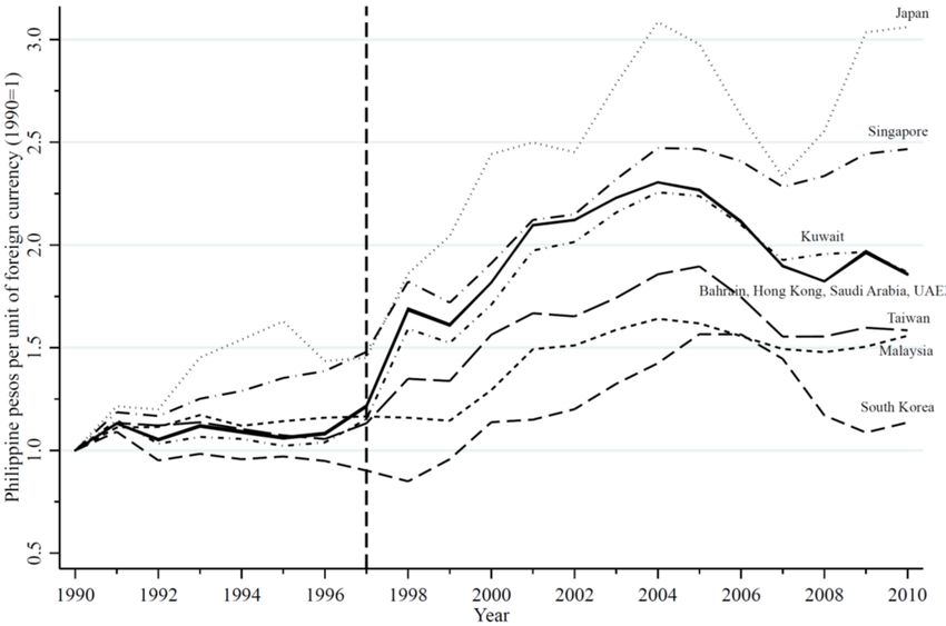
1   Introduction

How do earnings opportunities abroad affect development in origin areas of interna-
tional labor migrants? Consider effects in two contexts: in the domestic economy,
and in the international labor market. Domestically, migrant workers’ earnings may
loosen credit constraints on investments in education and enterprises in origin areas.
Domestic firms could benefit from access to better-educated workers, and increases
in local aggregate demand could stimulate local firm growth. Internationally, there
could also be gains. Improved migrant earnings opportunities could raise interna-
tional labor migration, and correspondingly increase aggregate earnings overseas.
If overseas earnings fund education investments back home, there could be further
gains over time. Populations with higher human capital may migrate at even higher
rates, and do so in higher-skilled, higher-paying overseas jobs.
    We examine the impacts of improvements in migrant earnings opportunities on
the origin areas of migrants in one of the world’s most important international mi-
gration source countries, the Philippines. Roughly one in four Philippine households
receive remittances from overseas migrants, so it is reasonable to examine potential
aggregate impacts on migrants’ origin areas. We exploit changes in migrant earn-
ings opportunities driven by the 1997 Asian Financial Crisis exchange rate shocks.
Locations across the Philippines had varied exposure to these shocks, because prior
to the crisis they differed in their rates of international migration, and also had var-
ied overseas destinations (whose exchange rate shocks were heterogeneous). Novel
administrative data from the Philippine government on migrant worker contracts
makes this study possible, by allowing us to estimate changes in migrant earnings
opportunities in sub-national areas (provinces).
    We study impacts over roughly a decade after the shock, looking separately at
impacts on the domestic economy (local labor market and firm outcomes), and inter-
national labor market outcomes. We find no large or statistically significant effects
on the domestic economy in origin areas, in terms of local labor force participation,
employment, household entrepreneurship, and domestic firm outcomes.
    By contrast, we find substantial positive effects on participation and performance
in the international labor market. Improvements in migrant earnings opportunities

                                           1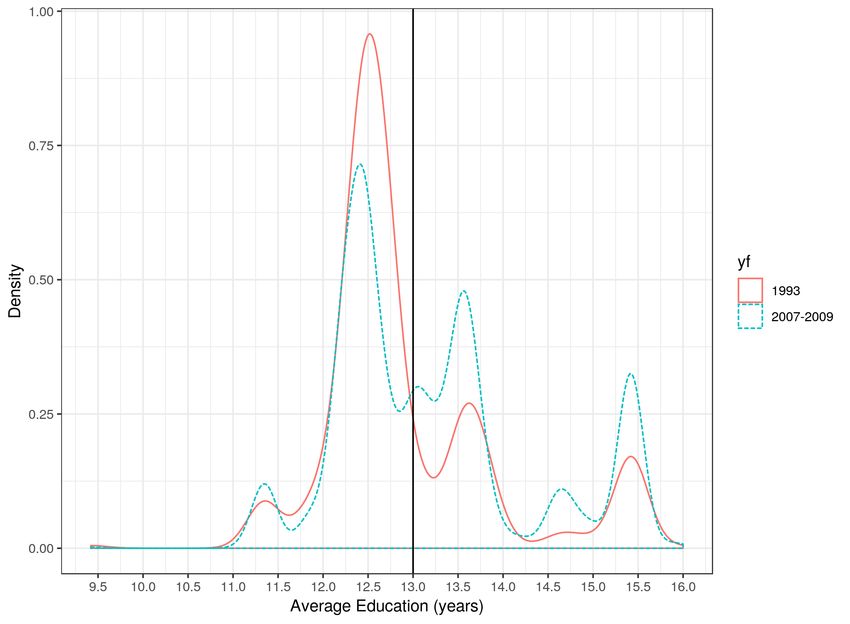
lead to increases in new departures for overseas jobs, and increases in migration for
higher-skilled overseas jobs. Correspondingly, there are substantial increases in av-
erage earnings per migrant. These increases in migration rates and in high-skilled,
high-wage migrant work add up to substantial gains in origin-areas’ aggregate over-
seas earnings. These gains in the international labor market are reflected in higher
aggregate wealth (higher asset ownership) in origin areas.
    The magnitude of impacts is nontrivial. A one-standard-deviation increase in
a province’s migrant earnings per capita (total annual migrant earnings divided by
population) increases the rate of new departures for international jobs by 38.7%
(0.38 std. dev.), the share of overseas jobs that are high-skilled by 11.6% (0.28 std.
dev.), and the provincial household asset index by 0.18 std. dev.
    Another aspect of the impacts bears notice: there is a substantial magnification
in the initial shock to migrant earnings over the subsequent decade. A one-standard-
deviation increase in the size of the initial migrant earnings per capita shock, or PhP
129, leads migrant earnings per capita in the province to be higher by PhP 1,263
(3.4% of per capita income) a decade later.1 In other words, each one-peso shock
to migrant earnings per capita in a province (driven by to the 1997 Asian Financial
Crisis exchange rate shocks) becomes 9.8 additional pesos a decade later.
    Is this dramatic magnification of the shock over time at all sensible? What could
explain such an effect? We write down a structural model to quantify potential
mechanisms behind the long-run effects we find. We are particularly interested in
how much of earnings gains might be due to increased educational investments,
which affect future migration and earnings.
    We start with a gravity model of migration (building on Eaton and Kortum
(2002), Bryan and Morten (2019) and Hsieh et al. (2019)), and augment it to allow
skill heterogeneity and skill investments. Workers make educational investments
to acquire skill and enter skilled occupations. Such investments are inhibited by
credit constraints, which may be alleviated by improvements in migrant earnings.
With dyadic (origin-destination) data on migration flows and wages, we estimate
the wage elasticity of migration, and dyad-level migration costs.
    Given the central role of skill acquisition in the model, we estimate impacts on
  1 All   monetary amounts in the paper are in real 2010 Philippine pesos. The 2010 exchange rate was 45 pesos to the USD.

                                                             2
educational investments. We find large positive effects: a one-standard-deviation
shock to migrant earnings increases years of schooling of 7-18 year-olds in the
province by 0.1 years (0.17 std. dev.), and of college-age individuals by 0.17 years
(0.15 std. dev.).
     Our parameter estimates and model can rationalize the magnitudes from our
reduced-form analysis. We quantify the importance of different channels in de-
termining long-run impacts, highlighting the education channel. We find that half
(50.1%) of the increase in the international migration rate is due to the education
channel. When it comes to the overall increase in migrant earnings per capita in the
population, 32% can be attributed to the education channel. Said differently, if the
initial improvement in migrant earnings opportunities had not affected household
educational investments, the impact on new migration and on migrant earnings a
decade later would only have been, respectively, half and two-thirds as large.
     All told, an exogenous improvement in migrant earnings opportunities in Philip-
pine provinces led to gains in a different realm than might have been expected. While
there were few identifiable gains in the domestic economy, origin areas saw substan-
tial gains in their participation and performance in the international labor market.
     Our work relates to research on the economic impacts of international migration
on migrants’ home areas. Prior work establishes that workers migrating internation-
ally experience substantial income gains (Gibson et al., 2010; Clemens et al., 2016),
and that improvements in migrant economic conditions have positive impacts on
their origin households (Yang (2006, 2008), Yang (2011)). We examine impacts on
outcomes of entire populations of migrant origin areas, not just the source house-
holds of current migrants. The focus on aggregate outcomes of origin areas is
relatively rare in the migration literature, owing to challenges in finding plausibly
exogenous variation in migration-related independent variables.2 A key concern in
such studies is that migrant earnings are not randomly assigned, so that observed
relationships with development outcomes may be due to omitted variables.3
    2 Previous studies on the aggregate impacts of international migration on origin areas include Orrenius et al. (2010), Lopez-

Cordoba (2005), Adams and Page (2005), Acosta et al. (2008), Dinkelman and Mariotti (2016), Barsbai et al. (2017), Abarcar
and Theoharides (2017), Theoharides (2018), and Theoharides (2019). Barham and Boucher (1998) and McKenzie and
Rapoport (2010) study impacts on income distribution in migrant home areas. Kinnan et al. (2019) examine impacts of
internal migration on origin areas in China.
    3 For example, areas with higher education levels could send more migrants, and also have better outcomes. Alternatively,

areas experiencing a negative shock might send more migrants overseas as a coping mechanism (Bazzi, 2017; Mahajan and

                                                               3
A key contribution of ours is to leverage a natural experiment that provides plau-
sibly exogenous variation in migrant earnings across localities. In addition, we ex-
pand the set of outcomes of interest beyond domestic economic outcomes, on which
prior work has tended to focus (Mendola, 2012; Hanson, 2009). Our novel migrant
contract data allows us to examine dynamic gains via changes in future migration.
We also examine impacts over an unusually long time-frame, a decade. Document-
ing dynamic gains due to increased education and resulting changes in international
labor outcomes requires such an expanded time-frame.
    We also contribute by estimating a structural model to provide insights beyond
the reduced-form analysis. We build on prior models (Bryan and Morten, 2019;
Burstein et al., 2018; Lagakos et al., 2019; Llull, 2018) by incorporating skill acqui-
sition and its consequences for migration and wages. We use the model to estimate
the impact of changes in migrant wages on migration probabilities for individuals
of given skill, and estimate how changes in skill levels affect migration. The model
helps us rationalize the magnitudes of effects, and quantify the role of educational
investments in yielding long-run gains.
    This paper also contributes to research on the impacts of migration on skill com-
position at origin. Our findings concord with studies finding that rather than leading
to a net loss of skilled individuals from the population (a “brain drain”), interna-
tional migration could increase skill levels by stimulating educational investments
(Stark et al. (1997), Mountford (1997), Shrestha (2017), Chand and Clemens (2019),
Batista et al. (2012), Docquier and Rapoport (2012)). These findings contrast with
studies finding reductions in schooling investments in response to migration oppor-
tunities (McKenzie and Rapoport (2011)). We add to this literature by emphasizing
that resulting increases in education in the population may create a virtuous cycle,
leading to more, higher-skilled, and higher-wage future migration.

2     Philippine Migration: Overview

The Philippines was the first country to facilitate large-scale temporary overseas con-
tract migration. Migration from the Philippines is largely temporary and legal, and
Yang, 2020), Mahajan and Yang (2020), so that migrant earnings might be negatively correlated with locality outcomes.

                                                            4
occurs through licensed, regulated private recruitment agencies. Filipino contract
workers oversas are widely referred to as OFWs (“Overseas Filipino Workers”). In
recent decades, increasing shares of the Philippine population have migrated, had a
household member migrate, or received migrant remittances (Appendix Table A2).
The fraction of the population currently overseas rose from 0.7% to 1.6% from 1990
to 2010. Over the same period, the fraction of households with an overseas migrant
member rose from 3.2% to 6.3%. Migrant financial support extends well beyond
their origin households: the share of households receiving remittances rose from
17.6% in 1991 to 26.0% in 2009.
The Philippines has perhaps the world’s most elaborate government bureaucracy
regulating international labor migration. The Philippine Overseas Employment Ad-
ministration (POEA) issues operating licenses to recruitment agencies and regulates
their activities. Due to concerns about worker abuses and human trafficking, re-
cruitment agencies are typically only allowed to recruit workers in approved office
locations. The Overseas Workers Welfare Administration (OWWA) works to en-
sure the well-being of OFWs and their families. It intercedes (via overseas consular
posts) for workers experiencing abuse or contract violations, repatriates workers in
conflict zones, assists OFW families in hardship, and facilitates the return and “rein-
tegration” of OFWs to the Philippines.
Filipinos migrate to a wide variety of destinations, and the choice of destination
varies substantially across origin areas. Table A1 shows the top twenty destinations
for all Filipino migrants prior to the Asian financial crisis. Other than Saudi Arabia
and Japan, no other destination accounts for more than 10% of migrants. There is
also substantial heterogeneity in the wages earned by migrants in different destina-
tions. Migrants to Saudi Arabia earn, on average, 306,000 Philippine pesos (Php)
per year, while the figure for migrants to Japan is Php 1.5 million. Within the Philip-
pines, emigration is more prevalent in certain provinces. Table 1 shows that, across
provinces, the average international migration rate for 25 to 64 year olds is 2.1%,
with a range of 0.1% to 7.3%.
53 Theoretical Framework
We write down a structural model to relate an initial migrant earnings shock with
educational investments and resulting future changes in migration and migrant earn-
ings. We build on recent gravity models of the flows of workers (Bryan and Morten
(2019); Hsieh et al. (2019)), which adapt Eaton and Kortum (2002) to model mi-
gration. Building on prior work, we endogenize skill investments, and allow for
skill-dependent migration and earnings. For identification, we exploit exogenous
changes in migrant earnings driven by exchange rate shocks. The model guides
our empirical specification, generates testable hypotheses, validates our empirical
findings, and quantifies underlying channels.
3.1 Migration Decisions
An individual i’s earnings widost varies across the province of origin o, the destina-
tion country d, their skill level s, and over t. It depends on migration costs τdot ,
exchange rates EXdt , destination specific ability draws qid , and destination specific
wage profiles wdst . Since recruitment agencies take a fraction of wages as their fees,
workers lose a percentage of their wages to migration cost. εdot is any unobservable
factor that makes migrants from origin o more productive in destination d.
widost = wdst EXdt (1 − τdot )qid εdot (1)
Here, τoo = 0. Like most of the literature, we assume ability is distributed multi-
variate Frechet with a shape parameter θ , as in Eaton and Kortum (2002).4 This
parameter determines the dispersion of skills across locations.5
( " #)
D
F(q1 , ....., qD ) = exp − ∑ q−θ
d (2)
d=1
4 Instead of a trade elasticity, as in Eaton and Kortum (2002), this will produce a migration elasticity: the elasticity between
the proportion of migrants and the destination wage.
5 Abilities may be correlated across locations with a correlation coefficient of ρ. For higher ρ, individuals that have
higher ability in location d also are more able in d 0 . In such cases, we can define θ̄ to measure the dispersion of skill, and θ
θ̄
would be a function of both the dispersion and correlation parameter: θ = 1−ρ . The distribution would be characterized by:
" #1−ρ
θ̄
− 1−ρ
F(q1 , ....., qD ) = exp − ∑D d=1 qd .
6Let πdost be the fraction of people of skill s from origin o who choose to work in d.
We can derive this share (the details of which are in Appendix D.1) to be:
(wdst EXdt (1 − τdot )εdot )θ
πdost = θ
(3)
∑k (wkst EXkt (1 − τkot )εkot )
Taking logs, we derive these gravity equations between origin-destination pairs:
" #
log πdost = θ log wdst +θ log EXdt +θ log (1−τdot )+log ∑ (wkst EXkt (1 − τkot )εkot )θ +θ εdot
k
(4)
3.2 Earnings Shocks and Human Capital Investments
Households choose schooling levels S when young, how much to borrow from the
future b̄, and work locations d when older. This location can be the home province
o or foreign countries. They maximize their two period utility: u(c1 ) + u(c2 ).
Period 1 consumption depends on wealth Y (including household migrant earn-
ings), the price of schooling p, and how much they borrow b from period 2. Period
2 consumption depends on earnings and unresolved period 1 debt with interest R:
c1io = Yio − po Sio + bio
c2io = wm
ido (s) − Ro bio , (5)
where wm ido (s) is the maximum wage at the end of the migration decision.
In equilibrium, the share of skilled s workers are `so and unskilled u workers
are `uo = (1 − `so ). If the average years of education for skilled workers is ed1 and
for unskilled is ed0 , then the average years of education in an origin o is simply:
So = `so ed1 + `uo ed0 .
Province-level earnings depend on the distribution of where workers work. The
short-run income change (due to exchange rate shocks) in the origin O depends on
the share of migrants in each destination:
∆EXkt
∆Yo = ∑ `sot ∑ πkost wkost , (6)
s k,o=O EXkt
7where wdost is the average wage in destination d for all workers of skill s from origin
o, πdost is the share of workers from o working in d, and ∆EX kt
EXkt is the exchange
rate shock. Equation (6) motivates our empirical specifications, where we leverage
variation in exchange rate shocks.6
We may expect that changes in migrant earnings help drive investments in hu-
man capital at home, for instance, by easing liquidity constraints for households.7
For reasonable assumptions on u(.) and w (for instance, wod (s) linear in s, and u(c)
continuous, increasing but at a decreasing rate), and for credit constrained house-
1
holds b̄ = 0, schooling will respond to shocks to migrant earnings: ∆So = 2p ∆Yo .
For ease of notation let us define: Ψ ≡ (ed1 − ed0 )2p, as the cost of becoming
skilled. The change in the share of skilled workers in an origin O will be:8
1 1 ∆EXkt
∆`sOt = ∆YO = ∑ `sot ∑ πkost wkost (7)
Ψ Ψ s k,o=O EXkt
3.3 Changes in Migration Flows in Response to the Shock
Migration flows from origin o to destination d depend on the probability of migrating
by skill level, and the share of workers who are skilled (`sot ) and unskilled (`uot ) :
πdost `sot + πdout `uot (8)
We can derive the changes in flows between origin o and destination d pairs. This
equation is important in that it drives the intuition behind our later analysis. We find
that the change in flows can be grouped into two components:
∆EXdt
∆ Flowsdot = ∆`sot (πdost − πdout ) + θ (`sot πdost + `uot πdout ) (9)
| {z } EXdt
Education channel in flows | {z }
Exchange rate channel in flows
−1
6 As 1
we show, from Frechet properties, we know wdost = wdst πdostθ Γ 1 − θ (1−ρ) , where Γ is the Gamma function.
7 In a similar manner, we may model liquidity constraints in investments in local enterprises. As we fail to find supportive
empirical evidence for this, we exclude it from the current setup for tractability purposes.
8 In Appendix D.2 we derive changes to human capital when there are no liquidity constraints or when there is no borrowing
possible. For the purposes of our study, we are agnostic about whether the education response is due to easing of liquidity
constraints or changing the returns to education. Some combination of the two is possible, as we discuss in the appendix.
Additionally, we note that if period 2 consumption is subjectively discounted, say at the rate β , then both the education and
β
skill-share response will be scaled by 1+β .
8First, skilled workers may have different migration probabilities than the un-
skilled. If the likelihood of migrating is higher for the skilled, then an increase in
the fraction of skilled workers will raise migration. If, on the other hand, most of
the demand from abroad is for low skill work, then the probability of migrating may
fall with skill. How skill changes affect flows are captured by the first term, ‘Educa-
tion channel in migrant flows.’ Intuitively, it is the product of two components: (a)
the education response to earnings ∆`sot , and (b) the skill-differential in migration
probabilities (πdost − πdout ).
Second, as exchange rates change favorably, there will be a migration response to
higher compensation. This depends on the Frechet parameter, which is the elasticity
of migration with respect to destination wages. Together, the size of the shock ∆EX dt
EXdt ,
the probabilities of migration `sot πdost + `uot πdout , and the responsiveness to shocks
θ , determine the change in migrant flows for a given skill level. This is what we call
the ‘Exchange rate channel in migrant flows.’
Similarly, the aggregate outflows of migrants from an origin o are summed over
various destinations, and follow the same intuition:
∆EXkt
∆ Flowsot = ∆`sot ∑ (πkost − πkout ) + θ ∑ (`sot πkost + `uot πkout ) (10)
k k EXkt
| {z } | {z }
Education channel in flows Exchange rate channel in flows
We use this set up to determine the importance of each channel, and quantify
their contributions. We need to estimate not just the change in education ∆`sot and
the migration elasticity θ , but also the baseline shares for ` and π which determine
how the shock in exchange rates propagates across different origins. Together, we
see how much of the changes in flows can be accounted for by the education and
exchange rate channels.
The equations also show that the change in flows is a function of the earnings
shock. This is true, not just for the exchange rate channel, but also for the education
channel. For instance, we know from Equation (7) for ∆`sot , that the education
channel directly depends on the migrant earnings shock:
9" #
1 ∆EXkt
Ψ ∑ `sot ∑ πkost wkost EXkt ∑ (πkost − πkout ) (11)
s k,o=O k
| {z }
∆Yo =Migrant Earnings Shock
3.3.1 Change in Earnings and Consumption Expenditure
The average earnings for the population in an origin O is a weighted average of
wages between origin o and destination d, which varies by skill s. The weights are
the fraction of the population in each skill group `sot , and the probability of working
in destination d given their skill level πdost :
!
∑ `sOt wdost πdost + ∑ `uOt wdout πdout = `sOt ∑ wdost πdost − ∑ wdout πdout + ∑ wdout πdout
d d d d d
(12)
Once again, the change in earnings per capita, will depend on what happens to
two different components, driven by: (1) the change in human capital , and (2) the
persistent change in exchange rates, which raises earnings and encourages flows to
favorable destinations. The education channel in earnings can be written as:
∆`sOt (∑ wdost πdost − ∑ wdout πdout ) (13)
d d
| {z } | {z }
avg skilled wage avg unskilled wage
Here, we know ∆`sOt is a function of the migrant earnings shock from Equation
(7). For ease of exposition, define β = (∑d wdost πdost − ∑d wdout πdout ) as the skill
premium. This allows us to rewrite the education channel contribution to the change
in earnings as:
!
β ∆EXkt
Ψ ∑ `sot ∑ πkost wkost EXkt (14)
s k,o=O
| {z }
∆Yo =Migrant Earnings Shock
The remaining change in earnings is driven by persistent changes in the exchange
rate. This ‘Exchange rate channel in earnings’ captures the increase in long run earn-
10ings, not simply due to the fact that better exchange rates directly increase earnings,
but also because they induce a greater flow of migrants (both skilled and unskilled)
to places with lucrative exchange rates. This contribution is:
! ! !
∆EX ∆EXdt ∆EXkt
∑ `sot wkost θ πdost EXdtdt + ∑ `uot wkout θ πdout
EXdt
= θ ∑ `sot ∑ πkost wkost
EXkt
k k s k,o=O
| {z }
∆Yo =Migrant Earnings Shock
(15)
In other words, this is θ ∆Y . Again, the migration elasticity plays an important
role in determining long-run earnings. Together, the overall change in earnings is:
β
+ θ ∆Y (16)
Ψ
There is intuition behind this relationship. First, a higher skill-premium β means
that as students get more educated (say, as liquidity constraints are eased), the more
the rise in earnings. Second, a lower cost of education Ψ means that easing liquidity
constraints has a larger impact on the education margin, as more children can easily
go to school. These two parameters determine the education channel’s contribution
in earnings. Third, a higher migration elasticity θ means that migration flows, and
thereby earnings, are more responsive to favorable exchange rates. This last param-
eter helps determine the importance of the changes in exchange rates in determining
long run earnings.
In the short run, total earnings and expenditures simply increase by ∆c1O = ∆YO .
In the long run, total migrant earnings, and as a result total household expenditures,
may increase by an amount greater than the initial gain in income:
β
∆ (c1O + c2O ) = ∆YO 1 + + θ > ∆YO (17)
Ψ
These overall changes in consumption expenditure reflect changes in long-run
consumption welfare. We use these derived lessons from our theoretical framework
to discipline our empirical analysis, interpret the coefficients of our reduced form
estimates, rationalize the magnitudes, and quantify the contribution of each of the
11different channels discussed.
4 Data Sources
We summarize data sources here, providing details in Appendix Section A.
4.1 Exchange Rate Shock Variables
Two administrative datasets from agencies of the Philippine government allow us
to calculate the two key province-level variables needed for our analysis: 1) the
earnings-weighted exchange rate shock, and 2) baseline (pre-shock) migrant earn-
ings per capita. These datasets are from the two agencies with primary charge over
overseas Filipino workers, OWWA and POEA (described in Section 2 above). The
first dataset is from OWWA. All Filipinos departing on overseas work contracts
are required to obtain OWWA membership prior to departure, and OWWA keeps
a detailed membership database that includes the migrant’s home address in the
Philippines. The second dataset, from POEA, provides data on migrant earnings.
POEA uses these data to verify that contracted wages meet minimum wage require-
ments. Both the OWWA and POEA data include name, date of birth, destination,
and gender, and so we match the two datasets using probabilistic matching in order
to determine the province of origin for all migrants in the POEA database. We com-
bine the POEA/OWWA data with monthly exchange rate data from Bloomberg LP
to construct the exchange rate shock.
4.2 Data on Outcomes
We use POEA/OWWA data from 1993, 2007, 2008 and 2009 on migrant contracts.
We focus on the numbers of new contracts and on their occupational characteris-
tics. The POEA/OWWA data categorize each occupational code into broad occupa-
tional groups (professionals, production workers, service workers), and we use these
groups when describing the change in the occupational distribution. In the parame-
terization of migration costs in the structural estimation, we also use information on
the locations of recruitment agency activity as recorded by the POEA.
12Data on years of schooling come from four rounds of the Philippine Census of
Population (1990, 1995, 2000, and 2010). The Census contains data on ownership
of a number of durable goods, access to utilities, housing quality, and land and home
ownership. We construct an index of household assets by taking the first principal
component of these variables (Filmer and Pritchett (2001)).9
The Philippine Census does not ask about employment status in all years, so we
use data from the Philippine Labor Force Survey (LFS), quarterly from 1992-2011,
to create a panel of labor supply outcomes. We examine province-level domes-
tic labor force participation rates for those aged 16 and above, employment rates
for children aged 10-15 (for whom labor force participation is not measured), and
household entrepreneurial work.
We use the Annual Survey of Philippine Business and Industry (ASPBI) to study
domestic firm production. We construct annual panel data (1988-2015) of province-
level means of manufacturing firm outcomes (revenues, exports, inventories, em-
ployment, hours worked, and compensation paid).
5 Estimation and Empirical Strategy
5.1 Gravity Equation Parameters θ and τod
Our gravity equation determines migrant flows from o to d. In Equation (4) the
unknown parameters are the migration elasticity θ and migration costs τod .
" #
log πdots = θ log wdst +θ log EXdt +θ log (1−τdot )+log ∑ (wkst EXkt (1 − τokt )εokt )θ +θ εdot
k
(4)
5.1.1 Estimating Migration Elasticities θ
To estimate the Frechet parameter, θ , first, we directly use Equation (4), and leverage
the exogenous exchange rate shocks. As such, the coefficient on log EXdt identifies
9 These asset data are only available in the 1990, 2000, and 2010 rounds of the Census. The loadings on the individual
variables are obtained from the principal component analysis for the 1990 data, and the resulting loadings are then used to
construct an asset index for 2000 and 2010. The principal component loadings can be found in Appendix Table A6.
13θ . We implement this in two different ways by structuring our data at the origin-
destination-skill level, and then simply at the destination-skill level. In the former
method we include origin-by-skill fixed effects and two-way cluster our errors at the
origin and destination level. In the latter method, we include the requisite skill fixed
effects and cluster our errors at the destination level.
For our second strategy, we recognize from the Frechet properties that, E(qd |d) =
− θ1
1
πdo Γ, where Γ = Γ 1 − θ (1−ρ) is the Gamma function. This allows us to derive
an earnings relationship to determine θ :
1
log wdost = log wdst −
log πdost + log Γ + εdot (18)
θ
As more and more workers from o move to d, it lowers the average wage, since
the marginal migrant has lower ability than the first set of migrants. We use earnings
data by origin, destination and skill-level of migrants. We include destination and
origin fixed effects, in a regression where our main independent variable is the log
of flows from origin to destination, and two-way cluster our errors at the origin-
destination pair level.
We estimate the models using Poisson pseudo-maximum likelihood (PPML),
which assumes that errors are uncorrelated with the exponential of the regressions.
Yet, one may think that εdot is correlated with log πdost . To get unbiased estimates,
we use instrumental variables, following Bryan and Morten (2019).10
Table A5 produces estimates of θ using the different methods. Our estimates of
θ lie between 3 and 3.7 across the different estimation procedures. Our IV-PPML
estimates are not statistically distinguishable from our PPML estimates of θ . We
use the estimate of 3.4 as our preferred estimate, but in sensitivity checks we vary it
for values between 2 and 7 when doing our model quantification exercises.
10 We construct a vector of all flows (and squared flows) to a destination from all other origins (i.e. excluding flows
from the origin of interest). We then use this vector Πdst−o to predict flows from the origin of interest πdost to the desti-
nation. Specifically, we create log Πdst−o to be a vector {log πd1st ...., log πdOst , (log πd1st )2 , .....(log πdOst )2 }. And then predict
\
log πdost = α1 log Πdst−o . We then run our 2SLS regression, where the first stage regresses log πdost on log \ πdost , and the sec-
ond stage implements Equation (18). We do this using IV-PPML with origin, destination and skill fixed effects, and bootstrap
our standard errors.
145.1.2 Estimating Migration Costs
In our framework, migration costs help drive the persistence in migration patterns,
and thereby the persistence in changes to migrant earnings. One reason underlying
persistence is the central role of recruitment agencies in international labor migra-
tion. Agencies enter into contracts with overseas employers to fill specified posi-
tions (e.g., nursing positions for a hospital in Qatar). Agencies interview potential
job applicants in licensed branches. Agencies therefore source job applicants from
particular localities, that tend to be persistent over time.
Recruitment agencies also specialize in placing workers in particular overseas
destinations where they have contacts and past experience. Overseas employers
choose agencies with whom they have worked before, or that have experience in the
same country and industry. The overseas destinations of workers placed by particu-
lar agencies therefore also tend to be persistent over time.
As a result of persistence in the Philippine areas of operation of recruitment
agencies, and of persistence in the overseas destinations served by particular agen-
cies, the costs of migrating from a particular Philippine origin location to a particular
destination country overseas are highly heterogeneous. We parameterize migration
costs between origin o and destination d as depending on the presence of recruitment
agencies, and their overseas areas of operation. Because agencies serve specific des-
tinations, the presence of an agency in origin o that serves destination d lowers the
cost of migrating from o to d. Furthermore, competition between agencies in origin
o placing workers in destination d should lower how much they charge potential
migrants, also lowering o to d migration costs.
If recruitment agencies do not rapidly spread across origins or destinations, then
the distribution of origin-destination flows may be strongly persistent over time (as
we empirically show later). This persistence in origin-destination flows may further
drive persistence in migrant earnings in the face of changes in exchange rates. We
parameterize the migration cost relationship in the following manner:
1
log (1 − τdot ) = λ1 # Rec Agendot + λ2 HHI Rec Agendot + εdot , (19)
where # Rec Agendot is the number of recruitment agencies in province o that send at
15least one migrant to destination d, and HHI Rec Agendot is the Hirschman-Herfindahl
Index for the competitiveness of the market that sends migrants from o to d.11
We use Equation (19) in conjunction with Equation (4). The migration costs
we estimate vary at the od-pair level. In Equationh (4), θ log wdst + θ logi EXdt are
absorbed by destination fixed effects µd , and log ∑k (wkst (1 − τkot ))θ εkot by origin
fixed effects, µo .
2
log πdot = µo + µd + θ λ1 # Rec Agendot + θ λ2 HHI Rec Agendot + εdot for t = T
(20)
In Equation (20), we control for both origin and destination fixed effects, and
migration costs are only identified by variation at the o − d pair level. This means
that whether the origin is a big city or a small town, or whether the destination is a
rich or a poor country, is not associated with the migration cost estimates.
That recruitment agencies play such a meaningful role in determining migration
flows can be seen by the raw data scatter-plot version of Equation (20) in Figure
A3. We residualize all the variables purging them of the origin µo and destination
µd fixed effects, and estimate the regression separately for 1993, and for the 2007-9
period. While this relationship is not meant to be causal, it quantifies the migration
costs for workers who wish to migrate from origin o to destination d. The relation-
ship between flows and agencies is strong, and also stable over the 16 year period
of our study. This stable and important role played by agencies may explain the un-
derlying heterogeneity in origin-destination flows, and the persistence in such flows
(and thereby migrant earnings) over time.
5.2 The Migrant Earnings Shock
As we show in Section 3, we expect migrant earnings to increase:
∆EXkt
∆Yo = ∑ `sot ∑ πkost wkost (6)
s k,o=O EXkt
We rewrite this relationship to facilitate estimation. Let baseline population in an
origin province (from the 1995 Census) be Popo , and the number of skilled workers
11 If haod is the share of workers sent by agency a to d, then HHIod = ∑a h2aod .
16in the province Lso . Let the number of skilled workers going from origin o, to
Lsot
destination d simply be Lsdo . This means that `sot ≡ Pop o
, and πdost ≡ LLsdot
sot
. We can
rewrite Equation (6) in the following manner:
Lsot Lskot ∆EXkt 1 ∆EXkt
∆Yo = ∑ ∑ wkost = ∑ ∑ Lskot wkost (6)’
s k,o=O Popo Lsot EXkt Popo s k,o=O EXkt
In terms of total migrant earnings for those from origin o and working in desti-
nation d, since wdot ≡ ∑s Lsdot wdost :
kt∆EX
∑ wko ∑k wko EXkt
∆Yo = k × (21)
Pop w
| {z o} | ∑k{z ko }
MigEarno ERshocko
We take this specification directly to the data, defining each of the components in
the product above in detail. As such, our causal variable of interest is the province-
level shock to migrant earnings per capita. This variable is the product of two di-
mensions of heterogeneity across provinces: baseline (pre-shock) migrant earnings
per capita MigEarno0 , and the earnings-weighted exchange rate shock ERshocko .
5.2.1 Earnings-weighted exchange rate shock
Because Filipino provinces differ in the destinations of their international migrants
(and their corresponding earnings), there was substantial heterogeneity in the earnings-
weighted exchange rate shocks experienced by different provinces following the
Asian financial crisis. The crisis was unexpected (Radelet and Sachs 1998), and so
migrants and their home areas should have been surprised by the shock. The crisis
led to the devaluation of numerous currencies throughout Southeast and East Asia,
including the Philippines’. As a result, the exchange rate vis-a-vis the Philippine
peso changed dramatically in many of the key destinations of Filipino migrants.
An appreciation of the exchange rate in a given destination provides a positive in-
come shock to Filipino migrants working there; each unit of foreign currency earned
abroad would be convertible to more Philippine pesos.
For each destination d, we measure the change in exchange rates between the
17twelve months preceding July 1997 and twelve months preceding October 1998:
∆EXd Average country d exchange rate from Oct. 1997 to Sep. 1998
= Average country d exchange rate from Jul. 1996 to Jun. 1997 −1 (22)
EXd
Exchange rate changes for the 20 major destinations of Filipino migrants are
presented in Table A1. Migrants in Saudi Arabia, Hong Kong, and the United Arab
Emirates experienced positive exchange rate shocks of approximately 50%. Mi-
grants in Malaysia and South Korea actually experienced slightly negative shocks.
We then calculate the average exchange rate shock for a Philippine province,
taking into account a province’s baseline share of migrant earnings across overseas
destinations. Let wdo be the total annual earnings of migrants from province o who
are in country d prior to the Asian financial crisis. The weighted-average exchange
rate shock for each o is the second term in Equation (21):
∆EX
∑k wko EXkk
ERshocko = (23)
∑k wko
In other words, the exchange rate shock for a province is the weighted aver-
age exchange rate change across those countries, with each country’s exchange rate
weighted by the fraction of a province’s migrant earnings in that country. Table 1
shows that this variable has a mean of 0.410 and a standard deviation of 0.045.
5.2.2 Baseline migrant earnings per capita
We estimate average earnings per migrant in the province using pre-shock contract
data, then multiply it by the number of migrants in each province from the 1995 Cen-
sus, obtaining total migrant wages for each province. We divide total migrant wages
by the province’s population to obtain a province’s pre-shock migrant earnings per
capita; the first term of Equation (21):
∑k wko
MigEarno = (24)
Popo
Table 1 shows summary statistics for MigEarno . The average is Php 4,263, and
the standard deviation is Php 3,275.
185.2.3 The shock to migrant earnings per capita
Our causal variable of interest is the province’s shock to migrant earnings per capita:
the product of the earnings-weighted exchange rate shock and baseline (pre-shock)
migrant earnings per capita. We construct this from demeaned component variables
(ERshocko and MigEarno ). It has a mean of -0.014 (std. dev. 0.129).
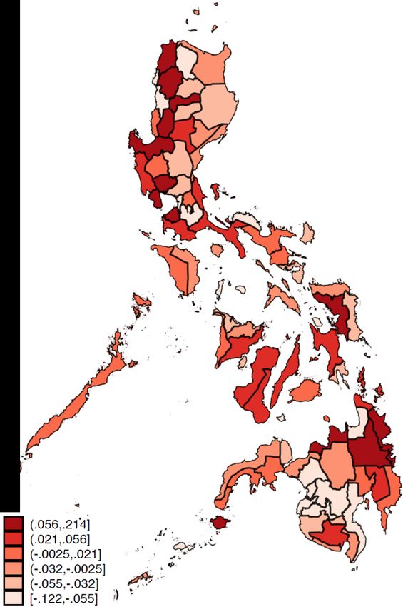
Figure A1 displays the spatial distribution of the residual shock to migrant earn-
ings per capita across Philippine provinces (after partialling out baseline migrant
earnings per capita and the earnings-weighted exchange rate shock). The shock ap-
pears to be evenly distributed across the country. All regions contain provinces with
a range of different shock values.12
5.2.4 Persistence of exchange rate shocks and migration patterns
There is temporal persistence in both the exchange rate shock and overseas migration
patterns, leading to persistence of the shock to province-level migrant earnings per
capita. Appendix Figure A2 shows the exchange rates for the top ten destinations.
The Asian financial crisis is denoted by the dashed line in 1997, after which there is
substantial dispersion of the exchange rates. The exchange rate shock is persistent
through the year 2010, as can also be seen Table A1 (columns 4 and 5).
In Appendix B.1, we formally test persistence of exchange rate shocks and over-
seas migrant destinations across provinces, and find strong evidence of both types
of persistence. The immediate (one-year) exchange rate shocks have a statistically
significant relationship with exchange rates up to 13 years after the Asian Financial
Crisis. In addition, the pre-shock (pre-1997) international migration destination pat-
terns of Philippine provinces have a positive and statistically significant relationship
with destination patterns more than a decade after the shock.
12 We explore what correlates with the shock in Appendix Table A7. In Column 1, we see that ERshock is larger (exchange
o
rate shocks are more positive) for provinces with high baseline migrant earnings per capita, lower baseline years of schooling,
lower female employment rates, and higher rural share of population. MigEarno (column 2) is higher for provinces with more
positive exchange rate shocks, higher share rural, and with higher asset index. For ERshocko × MigEarno , when migrant
earnings per capita and the exchange rate shock are not included as RHS variables, there is a statistically significant positive
association with years of schooling and female employment, and a negative one with the asset index. When we control for
the baseline level of migrant earnings per capita and the exchange rate shock, only the latter is statistically significant (it is
negative in sign), while the coefficients on the baseline province characteristics all decline substantially in magnitude, with
only average years of schooling being statistically significantly different from zero (and positive in magnitude).
195.3 Estimating the Impact of Migrant Earnings on Outcomes
The following is our regression specification:
yot = β0 + β1 ERshocko ∗ MigEarno ∗ Postt + β2 ERshocko ∗ Postt
+ β3 MigEarno ∗ Postt + αo + γt + φo ∗ Trendt + εot , (25)
yot is an outcome of interest for province o in period t. ERshocko is the earnings-
weighted exchange rate shock for province o (expression (23)). Postt is an indica-
tor for periods after 1997. MigEarno is annual migrant earnings per capita in the
province. αo are province fixed effects, γt are period fixed effects, and φo ∗ Trendt
is a province-specific linear time trend. εot is a mean-zero error term. Year and
province fixed effects account for time-invariant locality characteristics and com-
mon time effects. Province linear trends capture long-running linear changes in
outcomes specific to each province.13 Standard errors are clustered by province.
The regression specification includes ERshocko and MigEarno interacted with
Postt . We do not presume that ERshocko and MigEarno by themselves to be ex-
ogenous. The interaction terms with Postt account for changes from before to after
the shock related to these variables. Only the interaction between ERshocko and
MigEarno is taken to be exogenous. Therefore, our coefficient of interest is β1 on
the ERshocko ∗ MigEarno ∗ Postt term.
The identifying assumption is that a province’s shock to migrant earnings is un-
related to underlying trends in outcome variables. This is the parallel-trend assump-
tion underlying difference-in-difference estimates. In all results tables, we show
coefficient estimates without and with controls for heterogeneous province trends,
to gauge the robustness of results to their inclusion.
5.3.1 Human Capital, the Flow of Migrants, and Skilled Jobs
1
Our model predicts that schooling ∆So = 2p ∆Yo at the origin changes in response to
migrant earnings shocks. We estimate Equation (25) with years of education as the
13 For some outcomes, data are not available for enough periods to support province-specific linear time trends. In these
cases, we include a vector of pre-shock province-level controls interacted with a time trend (X p0 ∗ Trendt ). The variables in
X p0 are school attendance rate (age 7-18), female employment rate (age 25-64), male employment rate (age 25-64), share of
population rural, asset index, share of individuals (age 25-64) working in a household enterprise, and population.
20dependent variable. Equation (21) reveals that the shock affects the share of skilled
workers:
∆EXkt
1 1 ∑k wok ∑k wok EXkt
∆`sOt = ∆YO = × (7)’
Ψ Ψ Popo ∑k wok
| {z } | {z }
MigEarno ERshocko
We classify occupations to be high- or low-skill based on the average years of
education by occupation. We consider occupations where workers have 13 or more
years of education on average to be “high-skilled”.14
Next, we divide the occupations into the three largest categories in descending
order of skill: Professional jobs, production jobs, and service jobs. Professional jobs
(about 14% of contracts) are the highest skilled, with a mean monthly salary of Php
1357, while service workers (about 45% of our contracts) on average earn Php 297
a month. Our model predicts that the shock may shift migration flows toward high-
skill jobs as workers acquire more education (as emigration probabilities are higher
for skilled workers). We study the distribution of occupations in the POEA/OWWA
data to identify occupational upgrading.
Furthermore, our model suggests that the changes in migrant earnings will affect
the flows of migrants. This can be seen directly from Equations (10) and (11). Better
exchange rates drive migrant flows, and skill upgrading may amplify this further. We
test this hypothesis studying the number of new contracts in the POEA/OWWA data.
5.3.2 Long-run Migrant Earnings per capita and consumption
Persistent favorable exchange rate shocks will increase the stock of earnings, and the
flow of migrants going to places with such positive shocks. If the probability of em-
igrating is higher for skilled than unskilled workers, then the new flow of migrants
may be disproportionately skilled. This would raise the earnings per migrant, and
thereby the overall migrant earnings per capita in the long run. In Equation (16), our
model predicts that this shock to baseline migrant earnings will increase long-run
earnings due to both the increase in human capital accumulation (and occupational
upgrading), and the increased migrant outflows to favorable destinations. We test
14 Empirically, 13 years is a reasonable bifuracation point separating low from high skill. Figure A6 presents the density of
migrant education levels, which is bimodal with peaks just below and above 13 years.
21this hypothesis by examining long-run changes to migrant earnings per capita be-
tween 1993 and 2009.
These changes should also affect durable consumption in the long run, in the
manner that we describe in the model:
∆EXkt
∑k wok ∑k wok EXkt
β β
∆ (c1O + c2O ) = 1 + + θ ∆YO = 1 + + θ × (17)’
Ψ Ψ Popo ∑ k wok
| {z } | {z }
MigEarno ERshocko
We use the Census data to examine how durable consumption changes, by cre-
ating an asset index for households.
6 Empirical Results
6.1 Migrant earnings and flows of workers
We first examine impacts of the initial migrant earnings per capita shock on mi-
grant earnings per capita over the subsequent decade. We estimate regression Equa-
tion (25) where the dependent variable is province-level migrant earnings per capita
(total migrant earnings divided by province population, in thousands of real 2010
Philippine pesos). There is one pre-shock observation (1993) and three post-shock
observations (2007, 2008 and 2009) for each province.
These results are in the first row of Table 2, panel (a). The coefficient on the
migrant earnings shock is positive and statistically significant across sets of controls.
The effect is large in magnitude. Column 2’s coefficient estimate indicates that for
each one standard deviation increase in the initial migrant earnings per capita shock,
migrant earnings per capita are higher by nearly 1,263 pesos (9,810 pesos×0.129)
a decade later (equal to 3.4% of per capita income). The coefficient estimate of 9.8
indicates that the initial shock to migrant earnings is substantially magnified over
time: for each one-peso initial migrant earnings per capita shock, migrant earnings
per capita are nearly ten pesos higher a decade later.
What can account for such a considerable magnification over the subsequent
decade? Our theoretical framework guides us in unpacking the explanations.
22First, the shock also appears to have caused an increase in earnings per migrant.
In the second row of Table 2, panel (a), we show estimated coefficients on the mi-
grant earnings shock where the dependent variable is earnings per migrant. The
initial shock to migrant earnings per capita leads to substantially higher earnings per
migrant a decade later.
These increased earnings per migrant may reflect a few changes in origin provinces,
as suggested by our model. In panel (b), we show that the positive migrant earnings
shock led to meaningful increases in the education levels of the population. Coeffi-
cient estimates in column 2 indicate that a one-standard deviation migrant earnings
shock leads to 0.10 and 0.17 more years of schooling, for 7-18 year olds and 19-24
year olds, respectively. This increase in population skill levels may lead to higher
migration rates, and higher-skilled, higher-wage jobs abroad.
The shock did, in fact, lead to an increase in new migrant contracts, as can be
seen in panel (c). Theoretically, these increased flows are a result of better prospects
abroad given the persistent change in exchange rates, and occupational upgrading,
as provinces with positive shocks gain more education (as we will show, the high-
skilled are more likely to migrate).
Together, the education-driven occupational upgrading and the increased flow in
response to persistent favorable opportunities abroad drive the increase in migrant
earnings per capita. In Section 7 we quantify the role played by each of these chan-
nels in explaining the overall increase in migrant earnings.
In Figure 1a, we plot the pre-to-post change in migrant earnings per capita (av-
erage of 2007-9 minus 1993) against the migrant earnings shock. Both the x and
y-axis variables are residuals (partialled-out) from regressions on the exchange rate
shock (ERshocko ) and baseline migrant earnings per capita (MigEarno ). The non-
parametric regression plot also shows a positive relationship between the change in
migrant earnings per capita over the decade and the initial migrant earnings shock.
6.2 Assets
We turn to examining changes in assets, as a summary measure of household well-
being. We estimate equation (25) where the dependent variable is the average house-
hold asset index. Results are in Table 2, panel (d). The shock has a positive impact
23on the asset index, and is of substantial magnitude.
We also present nonparametric regression plots of the relationship between the
asset index and the shock. In Figure 1b, we plot the nonparametric relationship
of the pre-to-post change in assets (average of 2000 and 2010 minus 1990) against
the migrant earnings shock. Once again, both the y-axis and x-axis variables are
residuals (partialled-out) from regressions on the main effects of the exchange rate
shock (ERshocko ) and baseline migrant earnings per capita (MigEarno ). The plot
shows a positive relationship that appears approximately linear.
6.3 Schooling
Since human capital accumulation is central to our analysis, we examine changes
in schooling in detail. As our framework suggests, positive shocks to migrant earn-
ings could loosen financial constraints on investment in children’s schooling (Cox-
Edwards and Ureta, 2003; Yang, 2008; Gibson et al., 2011, 2014; Theoharides,
2019), and also change the expected return to education in the population at large.15
In Appendix Table A8, we present results from estimating regression Equation
(25) where the dependent variables are average years of completed schooling for var-
ious age and gender groupings. The unit of observation is the province by Census-
year. We find a positive effect for all children age 7-18 (row 1). Looking at narrower
age groups, we find positive and statistically significant effects for primary-school-
aged children (age 7-12) and for young adults (aged 19-24, tertiary schooling age).
For lower-secondary (age 13-15) and upper-secondary (age 16-18) children, regres-
sion coefficients are similar in magnitude, but are not consistently statistically sig-
nificantly different from zero. Results are similar when we examine impacts on
years of schooling separately for girls and boys. Comparing coefficient estimates
across columns 1 and 2, results tend to be stable (or increasing in magnitude) when
province-specific time trends are added to the regression.
Figure 2a displays a nonparametric regression of the relationship between years
of schooling for 7-12 year-olds and the shock. We plot the pre-to-post change (av-
erage across post-shock years minus average across pre-shock years) against the
15 As we discuss in Appendix D.2, positive migrant earnings shocks could raise schooling investments overall if the return to
education is perceived to rise (Chand and Clemens (2019), Shrestha (2017)), but could reduce schooling investments if returns
to education are seen to fall (McKenzie and Rapoport (2011)).
24migrant earnings shock. The nonparametric plot shows a positive relationship.
We also show a “placebo” experiment, taking advantage of the fact that we have
two observations of pre-shock data for this outcome (1990 and 1995). Figure 2b
displays a nonparametric regression plot that is analogous to the plot of panel (a),
except that the variable on the y-axis is the change in the pre-shock period (1995
minus 1990). This is a partial test of the parallel-trend identification assumption.
The plot supports this assumption: no positive relationship between the pre-shock
change in schooling and the shock is apparent.16 In Table A10 we formally test for
pre-trends across all these education outcomes by looking at the changes between
1990 and 1995. We fail to reject the null of no differential pre-trends across all our
specifications in panel (a) on education outcomes.
6.4 Skills and occupational upgrading
The increase in schooling levels may change the flow and composition of migrants.
Workers with more education find it relatively easier to find work abroad.17 These
workers may also be more likely to find higher-paying jobs. Alternatively, workers
with more education may have more employment prospects at home, leading to
negatively selected migration following exchange rate shocks.
For ease of exposition, we classify each detailed occupation code as skilled or
unskilled. Figure A6 shows two modes that appear around the 13 year mark, so we
use 13 years as a threshold to divide the occupations.18
Panel (a) of Table 3 shows these results for the full population (including mi-
grants) and migrant workers separately. First, it is clear that migrant workers are
about twice as likely to be skilled than the general population. The migrant earn-
ings shock increases the share of skilled workers in both the full population and
the migrant population, and the coefficients are statistically significant. Column 2
shows a that a one-standard-deviation shock leads to a 0.6 percentage point increase
(0.0464×0.129) in the share skilled in the full population. Relative to a mean of 17.3
16 Similar “true” and “placebo” experiments are shown in Appendix Figures A4 and A5, for 7-18 year-olds and 19-24 year
olds, respectively. The patterns are very similar to those of Figure 2: there is a positive relationship Panel A (true experiment)
and no relationship in Panel B (placebo experiment).
17 In our model this depends on the relative probabilities of skilled and unskilled migrant flows, π
dost and πdout .
18 Our results are not sensitive to varying this cutoff. Those with 12 years are likely to have a vocational degree. Those with
14 years are likely to have finished college.
25You can also read