Global Warming and Terrestrial Biodiversity Decline
←
→
Page content transcription
If your browser does not render page correctly, please read the page content below
WWF2037 Cover.QX   8/14/00   5:23 PM   Page 1

                                                Global Warming
                                                     and
                                                 Terrestrial
                                                    Biodiversity Decline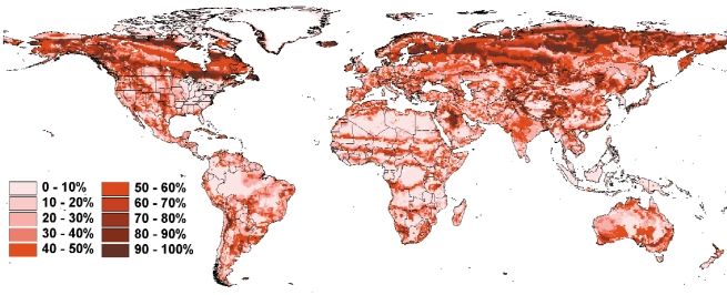
Global Warming and Terrestrial Biodiversity Decline
Published September 2000 by WWF-World Wide Fund For Nature (Formerly World                   by                                            and
Wildlife Fund), Gland, Switzerland. WWF continues to be known as World Wildlife Fund
in Canada and the US. Any reproduction in full or in part of this publication must           Jay R. Malcolm                                Adam Markham
mention the title and credit the above-mentioned publisher as the copyright owner.
© text 2000 WWF. All rights reserved.                                                        Faculty of Forestry, University of Toronto,   Clean Air-Cool Planet, 100 Market Street,
The material and the geographical designations in this report do not imply the               Toronto, ON, Canada M5S 3B3                   Suite 204, Portsmouth, NH 03801
expression of any opinion whatsoever on the part of WWF concerning the legal
status of any country, territory, or area, or concerning the delimitation of its frontiers   416.978.0142                                  603.422.6466
or boundaries.                                                                               (jay.malcolm@utoronto.ca)                     (amarkham@cleanair-coolplanet.org)

                                                                                                                                           A Report Prepared for WWF

                                                                                                                                           August 2000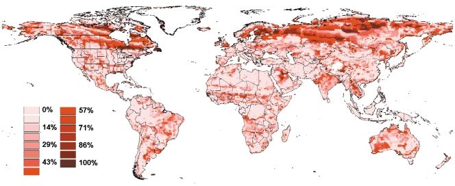
Table of Contents              contents                     executive summary
                                                                         Executive Summary

                             Executive Summary
                             Introduction                  1
                                                               ii
                                                                         P   ast efforts to model the potential effects of greenhouse warming on global ecosystems
                                                                             have focussed on flows of energy and matter through ecosystems rather than on the
                                                                         species that make up ecosystems. For this study, we used models that simulate global climate
                             Methods              5                      and vegetation change to investigate three important threats to global terrestrial biodiversity:

                             Results           10                            1) Rates of global warming that may exceed the migration capabilities of species
                                                                             2) Losses of existing habitat during progressive shifts of climatic conditions
                             Discussion & Conclusions               13
                                                                             3) Reductions in species diversity as a result of reductions in habitat patch size.
                             Tables          18
                                                                         We also analyzed the effects that major natural barriers such as oceans and lakes, and human-
                             Figures           24                        caused impediments to migration, including agricultural land and urban development, might
                                                                         have on the ability of species to move in response to global warming.
                             Acknowledgements                  32
                                                                         Seven climate models (general circulation models or GCMs) and two biogeographic models
                             Endnotes             32
                                                                         were used to produce 14 impact scenarios.1 The models do not provide information on biodi-
                                                                         versity per se, but instead simulate future distributions of major vegetation types (biomes) such
                                                                         as boreal coniferous forest and grassland. We were able to use the models to indirectly investi-
                                                                         gate potential biodiversity change in several ways:

                                                                               • To measure the rates of migration that greenhouse warming might impose on species,
                                                                                 we calculated the rates at which major vegetation types would need to move if they
                                                                                 were to be able to successfully keep up with climate change. The shifts of biome
                                                                                 boundaries under the different climate scenarios were used as proxies for shifts in the
                                                                                 distributional boundaries of plant species.

                                                                               • To measure the potential loss of existing habitat, we compared current vegetation dis-
                                                                                 tributions with those projected for the future under the various scenarios, and quanti-
                                                                                 fied the areas of change.

                                                                               • Finally, by making use of well-established relationships between habitat patch size and
                                                                                 species richness, we investigated the potential for species loss due to predicted reduc-
                                                                                 tions in the area of habitat patches remaining after warming.

                                                                         The fate of many species in a rapidly warming world will likely depend on their ability to per-
                                                                         manently migrate away from increasingly less favorable climatic conditions to new areas that
                                                                         meet their physical, biological and climatic needs. Unfortunately, the ability of species to
                                                                         migrate is generally poorly understood so it is difficult to determine just how serious the
                                                                         impacts of climate change might be on biodiversity. Much of our knowledge about potential
                                                                         for rapid migration of species comes from fossil evidence of how forests re-colonized previous-
                                                                         ly glaciated areas after the last ice age. However, scientists are not in agreement as to whether
                                                                         the rates attained at that time are the maximum attainable rates, or whether at least some
                                                                         species could move faster if necessary. Therefore, instead of attempting to predict how fast
                                                                         species and biomes might be able to move, we analyzed how fast they might be required to
                                                                         move in order to keep up with projected warming.

ii   Global Warming and Terrestrial Biodiversity Decline                                                                                                                     iii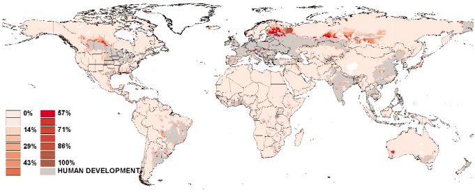
We calculated “required migration rates” (RMRs) for all terrestrial areas of the globe. RMRs of              • The barriers to migration represented by human population density and agriculture
                             greater than 1,000 m/yr were judged to be “very high” because they are very rare in the fossil                 were also regionally influential, particularly along the northern edges of developed
                             or historical records. We compared RMRs under scenarios where CO2 doubling equivalent was                      zones in northwestern Russia, Finland, central Russia and Central Canada.
                             reached after 100 years, and after 200 years, in order to assess the influence of the rate of
                                                                                                                                          • In addition to imposing high RMRs on species, global warming is likely to result in
                             global warming on the vulnerability of species. In fact, even relatively optimistic emissions
                                                                                                                                            extensive habitat loss, thereby increasing the likelihood of species extinction. Global
                             scenarios suggest that CO2 concentrations in the atmosphere are likely to have doubled from
                                                                                                                                            warming under CO2 doubling has the potential to eventually destroy 35% of the
                             pre-industrial levels around the middle of this century and will almost triple by 2100. This
                                                                                                                                            world’s existing terrestrial habitats, with no certainty that they will be replaced by
                             means that the RMRs reported here are likely to be on the conservative side and that species
                                                                                                                                            equally diverse systems or that similar ecosystems will establish themselves elsewhere.
                             may need to move even faster than reported here. Our results indicate that climate change has
                             the potential to radically increase species loss and reduce biodiversity, particularly in the high-          • Russia, Sweden, Finland, Estonia, Latvia, Iceland, Kyrgyzstan, Tajikistan, and Georgia
                             er latitudes of the Northern Hemisphere.                                                                       all have more than half of their existing habitat at risk from global warming, either
                                                                                                                                            through outright loss or through change into another habitat type.

                                                                                                                                          • Seven Canadian provinces/territories – Yukon, Newfoundland and Labrador, Ontario,
                             Summary of key findings
                                                                                                                                            British Columbia, Quebec, Alberta and Manitoba - have more than half their territory
                             Specific conclusions:                                                                                          at risk.

                                     • All model combinations agreed that “very high” required migration rates or RMRs                    • In the USA, more than a third of existing habitat in Maine, New Hampshire, Oregon,
                                       (≥1,000 m/yr) were common, comprising on average 17 and 21% of the world's sur-                      Colorado, Wyoming, Idaho, Utah, Arizona, Kansas, Oklahoma, and Texas could
                                       face for the two vegetation models.                                                                  change from what it is today.

                                     • RMRs for plant species due to global warming appear to be 10 times greater than                    • Local species loss under CO2 doubling may be as high as 20% in the most vulnerable
                                       those recorded from the last glacial retreat. Rates of change of this magnitude will like-           arctic and montane habitats as a result of climate change reducing the size of habitat
                                       ly result in extensive species extinction and local extirpations of both plant and animal            patches and fragments. Highly sensitive regions include Russia’s Taymyr Peninsula,
                                       species.                                                                                             parts of eastern Siberia, northern Alaska, Canadian boreal/taiga ecosystems and the
                                                                                                                                            southern Canadian Arctic islands, northern Fennoscandia, western Greenland, eastern
                                     • High migration rates were particularly concentrated in the Northern Hemisphere,
                                                                                                                                            Argentina, Lesotho, the Tibetan plateau, and southeast Australia. These losses would
                                       especially in Canada, Russia, and Fennoscandia. Despite their large land areas, an aver-
                                                                                                                                            be in addition to those occurring as a result of overall habitat reduction.
                                       age of 38.3 and 33.1% of the land surface of Russia and Canada, respectively, exhibited
                                       high RMRs.

                                     • The highest RMRs are predicted to be in the taiga/tundra, temperate evergreen for-           General conclusions:
                                       est, temperate mixed forest and boreal coniferous forest, indicating that species
                                                                                                                                          • It is safe to conclude that although some plants and animals will be able to keep up
                                       dependent on these systems may be amongst the most vulnerable to global change.
                                                                                                                                            with the rates reported here, many others will not.
                                     • Even halving the rate of global warming in the models did little to reduce the areas
                                                                                                                                          • Invasive species and others with high dispersal capabilities can be predicted to suffer
                                       with high RMRs.
                                                                                                                                            few problems and so pests and weedy species are likely to become more dominant in
                                     • Water bodies, such as oceans and large lakes, that can act as barriers to migration were             many landscapes.
                                       shown to be significant factors in influencing RMRs in some regions, especially on
                                                                                                                                          • However, in the absence of significant disturbance, many ecosystems are quite resistant
                                       islands such as Newfoundland, and peninsulas such as western Finland.
                                                                                                                                            to invasion and community changes may be delayed for decades.

iv   Global Warming and Terrestrial Biodiversity Decline                                                                                                                                                                              v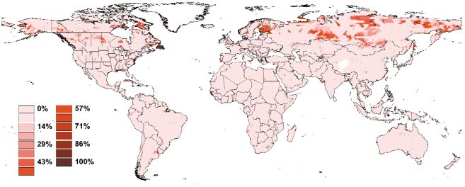
introduction
                                                                                                                                     Introduction

                                      • Global warming is likely to have a winnowing effect on ecosystems, filtering out those
                                        that are not highly mobile and favoring a less diverse, more “weedy” vegetation or sys-
                                        tems dominated by pioneer species.
                                                                                                                                     C     limate plays a primary role in determining both the geographic distributions of organ-
                                                                                                                                           isms and the distributions of the habitats upon which they depend. In the past, direction-
                                                                                                                                     al climate change has resulted in significant shifts in the distributions of species (Davis 1986).
                                                                                                                                     Temperate tree species, for example, migrated at rates of tens of metres per year or more to
                                      • Non-glaciated regions where previous selection for high mobility has not occurred
                                                                                                                                     keep up with retreating glaciers during the Holocene (Huntley and Birks 1983). If allowed to
                                        among species may suffer disproportionately. Therefore, even though high RMRs are
                                                                                                                                     continue, greenhouse warming is similarly expected to result in significant shifts in vegetation
                                        not as common in the tropics, there may still be a strong impact in terms of species loss.
                                                                                                                                     types. To illustrate, a recent effort to model the effect of a doubling of greenhouse gas concen-
                                      • Some species have evolved in situ and may fail to migrate at all.                            trations on vegetation projected shifts in major vegetation types in 16-65% of the land area of
                                      • Future migration rates may need to be unprecedented if species are to keep up with           the lower 48 U.S. states, depending on the exact combination of models used (VEMAP
                                        climate change.                                                                              Members 1995). While climatic shifts of this sort have been observed in the past, and can be
                                                                                                                                     expected in the future even in the absence of human activities, the rate of greenhouse warm-
                                      • Human population growth, land-use change, habitat destruction, and pollution stress-         ing appears likely to be unprecedented in at least the last 100,000 years, with a doubling of
                                        es will exacerbate climate impacts, especially at the pole-ward edges of biomes.             greenhouse gases concentrations and associated warming expected to occur within a mere 100
                                      • Increased connectivity among natural habitats within developed landscapes may help           years. Although poorly understood, the rapidity of the change could have important implica-
                                        organisms to attain their maximum intrinsic rates of migration and help reduce               tions for terrestrial biodiversity, with the possibility of significant species loss (Malcolm and
                                        species loss.                                                                                Markham 1996, 1997).

                                      • However, if past fastest rates of migration are a good proxy for what can be attained in     With improved abilities to model future global climate and vegetation change comes the possi-
                                        a warming world, then radical reductions in greenhouse gas emissions are urgently            bility to investigate in more detail this threat to global biodiversity. Unfortunately, this impor-
                                        required in order to reduce the threat of biodiversity loss.                                 tant task as yet has received little attention. Instead, research has tended to focus on functional
                                                                                                                                     properties of ecosystems, such as the ways in which they process energy and matter (e.g.
                             In conclusion, this study demonstrates that rapid rates of global warming are likely to
                                                                                                                                     VEMAP Members 1995). The few attempts to model processes acting at the species level have
                             increase rates of habitat loss and species extinction, most markedly in the higher latitudes of
                                                                                                                                     been restricted to one or a few localities and a small subset of the flora and fauna. In this
                             the Northern Hemisphere. Extensive areas of habitat may be lost to global warming and
                                                                                                                                     report, we examine the question of global biodiversity decline. In particular, we use global
                             many species may be unable to shift their ranges fast enough to keep up with global warming.
                                                                                                                                     climate and vegetation models to investigate three possible threats to global biodiversity:
                             Rare and isolated populations of species in fragmented habitats or those bounded by large
                             water bodies, human habitation and agriculture are particularly at risk, as are montane and                   1) Warming that exceeds the migrational capabilities of species
                             arctic species.                                                                                               2) Losses of habitat during progressive shifts of climatic conditions

                                                                                                                                           3) Reductions in species diversity through reductions in habitat patch size.

                                                                                                                                     Although the models do not provide direct information on changes in species diversity
                                                                                                                                     (rather, they map distributions of vegetation types), we can nevertheless use them in a heuris-
                                                                                                                                     tic fashion to indirectly examine these threats. For example, to assess the migration speeds
                                                                                                                                     that species might have to achieve in order to keep up with shifting climatic conditions, we
                                                                                                                                     can measure the speed of shifting vegetation types. Similarly, habitat losses and reductions in
                                                                                                                                     the areas of habitat patches can be quantified by comparing current and future vegetation
                                                                                                                                     maps and quantifying areas of change. Although indirect, these methods provide powerful
                                                                                                                                     tools to investigate possible threats to biodiversity.

vi   Global Warming and Terrestrial Biodiversity Decline                                                                                                                                                                                   1
Rapid Climate Shifts Perhaps most importantly, how will human behaviour influence these future rates? Are the
rates substantially elevated in areas where habitat has been lost through development? What is
Although species have inherent abilities to respond to climatic shifts through population
the relationship between the rate of greenhouse warming and future migration rates?
processes such as birth, death, and dispersal, the speed at which they can respond is limited. If
climatic conditions shift quickly enough, slower moving species may be left behind, especially
if human activities have destroyed and fragmented existing habitat. As shown schematically in Habitat Loss
Figure 1A, as climatic conditions shift, so will the conditions for successful growth and repro-
duction of many species. In order to occupy newly-suitable areas, species must migrate from Worldwide, habitat loss has been identified as a primary cause of species extinction and endan-
existing source populations. Although many species have migrated in the past in response to germent. Climate change can be expected to result in shifts in habitat conditions, with the
changing climates, the shifts imposed by global warming may exceed the capabilities of many eventual loss of existing habitats in many areas (Figure 2B). New habitats may reappear else-
species. For example, Dyer (1995) modeled migrations of trees dependent on wind or bird where, but in many cases only if the requisite biotic (living) elements are able to track the abi-
dispersal and concluded that even in relatively undisturbed landscapes, migration rates fell otic (physical) change. Appropriate habitat usually depends on both abiotic and biotic ele-
short of projected global warming range shifts by at least an order of magnitude. Other studies ments, although the importance of the two varies from one species to another. If climatic con-
have similarly concluded that future plant migration could lag behind climatic warming, ditions shift, but suitable biotic elements fails to migrate, then new habitat areas may be of
resulting in altered relationships between climatic conditions and species distributions, lower quality for many species. An example would be the failure of trees to migrate pole-ward
enhanced susceptibility of plant communities to natural and anthropogenic disturbances, and despite the fact that suitable conditions for forest cover have shifted towards higher latitudes.
eventual reductions in species diversity (Davis 1989, Overpeck et al. 1991). Added to the prob- Species dependent on forest conditions for food, nesting, or cover would be unable to utilize
lem of rapidly shifting climatic zones are habitat losses in human-dominated landscapes, with the new area.
current landscapes providing fewer possibilities for migration than historic ones. Several studies have used global vegetation models to map areas of possible vegetation change.
The possibility that global warming might require relatively high migration rates has serious Here, we expand on previous efforts by simultaneously investigating vegetation change for a
implications, especially if the mismatch between climatic warming and migration rates affects large suite of global climate and vegetation models. We were interested in the consistency of
species such as trees that disproportionately affect ecosystem properties. One potential conse- the patterns of change among models and in whether or not patterns of habitat loss were con-
quence of high migration rates, for example, is a decrease in the ability of forests to store car- centrated in particular regions of the globe.
bon from the atmosphere and hence a decrease in their ability to ameliorate greenhouse
warming. In a scenario in which trees were perfectly able to keep up with global warming,
Declines in Patch Area and Associated Species Loss
Solomon and Kirilenko (1997) observed that the warming associated with a doubling of
atmospheric CO2 resulted in a 7-11% increase in global forest carbon. In a contrasting sce- The rate of climate change is expected to vary from one region to another, with some regions
nario in which they assumed zero migration, a 3-4% decline in global forest carbon was undergoing less rapid change than others. However, even if the climate (and habitat) in an
observed. Kirilenko and Solomon (1998) obtained a similar result when they used past tree area remains relatively unchanged, changes in the surrounding landscape may have indirect
migration rates as estimates of potential future migration rates and found that a large portion effects. In particular, if the extent of a habitat patch declines over time, then declines in
of the earth became occupied by plant assemblages that were less diverse. Sykes and Prentice species diversity within the patch can be expected. This species loss will arise from a combina-
(1996) also investigated an all-or-none migration scenario at a site in southern Sweden. tion of factors, including reduced population sizes of the various species that inhabit the patch
Compared to perfect migration, zero migration resulted in fewer tree species, lower forest bio- and reduced diversity of micro-habitat types within the patch. A considerable body of research
mass, and increased abundance of early successional species. over the past decades has identified a strong relationship between habitat area and species
richness. Following MacArthur and Wilson's (1967) development of the Theory of Island
Although several studies have investigated the capabilities of species to migrate in response to
Biogeography, which predicted that species diversity would decrease with island size, ecologists
global warming, none has investigated in detail the overall rates of migration that global warm-
began applying similar concepts to “habitat islands,” such as forest patches, lakes, and moun-
ing might impose. How do these possible future rates compare with past rates? Are migration
tain tops. Empirical evidence has shown that if species richness and patch area are plotted
rates uniform across the surface of the planet or are they particularly high in some regions?
against each other, species richness strongly increases with area.2 A classic application of this
2 Global Warming and Terrestrial Biodiversity Decline 3Methods methods
observation to the problem of global warming was provided by McDonald and Brown (1992). Quantifying Threats to Biodiversity
These authors used temperature gradients to investigate the future distributions of high alti-
To investigate these threats to biodiversity, we employed linked global climate and vegetation
tude habitats in isolated mountain ranges of the Great Basin of the U.S. Southwest. This area
models. In combination, these models can be used to map the potential future distributions of
of sagebrush desert is interrupted at irregular intervals by isolated mountain ranges that pro-
major vegetation types (biomes). Given any atmospheric CO2 concentration, the climate mod-
vide the cool moist conditions required to support a relictual boreal mammal fauna. The lim-
els simulate climatic conditions, and given this simulated climate, the vegetation models deter-
its of this cooler habitat can be mapped quite accurately by using temperature, hence the
mine potential vegetation types. Two sets of models were run: a “control” set in which atmos-
authors could compare current and projected future distributions of the habitat by comparing
pheric CO2 concentrations approximated recent historical conditions (e.g. 1961-1990) and a
current and future temperature maps. Possible changes in species richness could then be
“future” set in which atmospheric CO2 concentrations were twice as high. The global climate
investigated based on the relationship between habitat area and species richness. Under mean
models, known as General Circulation Models (GCMs), are detailed computer simulations that
warming of 3 oC, McDonald and Brown (1992) observed that montane ecosystems decreased
model three-dimensional representations of the earth's surface and solve the systems of equa-
in size due to upslope migration, with individual ranges losing anywhere between 35 and 96%
tions that govern mass and energy dynamics. They suffer from coarse grid sizes and numerous
of their original boreal habitat. Based on the species-area relationship, different mountain
simplifying assumptions; however, they have met with considerable success in modeling global
ranges lost between 9 and 62% of their boreal mammal species. Three of fourteen mammal
climatic patterns (e.g. Hasselmann 1997, Houghton et al. 1996, Kerr 1996). The vegetation
species were predicted to go extinct across the entire Great Basin.
models make use of ecological and hydrological processes and plant physiological properties to
Surprisingly, this approach has not been undertaken over larger areas. Here, we use their predict potential vegetation on upland, well-drained sites under average seasonal climate condi-
approach, albeit at a coarser scale of resolution, and apply it at the global scale. We were par- tions. A simulated mixture of generalized life forms such as trees, shrubs, and grasses that can
ticularly interested in the possibility of biodiversity loss in alpine and arctic habitats. As tem- coexist at a site is assembled into a major vegetation type (or biome) classification (Neilson et al.
peratures rise and the cool conditions required by these habitats shift upward and pole-ward, 1998). These models are termed “equilibrium” models because they model the vegetation that
reductions in area are expected. Are these decreases likely to be accompanied by significant would be expected to occur at a site once both climate and vegetation change at the site have
species loss? stabilized. A standardized series of climate and vegetation models such as that used in the
VEMAP project (VEMAP Members 1995) was not available at the global scale; however, 14 com-
binations of models were available to us. These included seven global climate models, including
both “older” and “newer” generation models 3, and two global vegetation models (MAPSS
[Neilson 1995] and BIOME3 [Haxeltine and Prentice 1996])4. The state of climate and vegeta-
tion modeling is not such that the model outcomes can be viewed as predictions (VEMAP
Members 1995). Rather, the models represent a range of possible future outcomes as envisioned
by different groups of scientists. Uncertainties concerning the best ways in which to model cli-
mate and vegetation are considerable, hence our use of this range of possibilities. However, it is
important to note that the uncertainty concerning the effects of increasing greenhouse gas con-
centrations should not be confused with an increased possibility of the “no change” option.
More extreme change than predicted is as likely as less extreme change.
A Heuristic Approach to Modeling Biodiversity Change
Any attempt to model the effect of climate change on all of the myriad species in an ecosystem
would be a very detailed and difficult undertaking. Basic information is often lacking, for
example, where species occur and how quickly they might respond to change. At the global
level, information gaps become even more serious; for example, it is not yet possible to accu-
rately map species ranges across the entire planet for any group of organisms, with the possi-
ble exception of birds. Equally problematic are the complex sets of interactions among
species, which often determine how they respond to change. An illustrative example is the dis-
tinction between the “fundamental” and “realized” niches of a species. The former represents
the possible range of physical conditions which the species can occupy, whereas the latter rep-
4 Global Warming and Terrestrial Biodiversity Decline 5resents the observed set of conditions that it actually occupies under the influence of addition- area where the species already occurred. The simplest assumption is that it came from the
al factors such as predation, competition, etc. Predicting the effect of global warming on physi- nearest possible locality in the species former range. Note that where current and future vege-
cal conditions is relatively straightforward, but disentangling the interaction of both physical tation types stay the same (the region labeled “a” in Figure 1A), the species would not have to
and biotic changes is enormously difficult. migrate at all, and the required migration rate would be zero. An average required rate for a
species thus includes these areas of zero migration.
Nevertheless we can apply general ecological principles to investigate possible biodiversity
change. In this paper, rather than attempting to model each species, we apply a broader brush Based on IPCC estimates (Houghton et al. 1996), we assumed that the doubled CO2 climate
and, as detailed below, take a more heuristic approach. A good example of this sort of would occur in 100 years. This assumption is based on an IPCC midrange emission scenario,
approach is provided by McDonald and Brown (1992) who used empirical species-area rela- “medium” climate sensitivity (2.5 oC), and sulphate aerosol cooling. Some transient model
tionships to study biodiversity loss as described above. runs suggest that 2 x CO2 forcing may be reached over a considerably shorter time period (see
references in Solomon and Kirilenko 1997); hence, our migration rates may be conservative.
A final important factor to consider is the breadth of the biome definitions. The two vegetation
Migration rates
models used somewhat different definitions of a “biome” and also divided up major biome
The factors affecting the ability of organisms to migrate in response to climate changes are not types in different ways. Specifically, BIOME3 modeled 18 biome types, whereas MAPSS modeled
well understood even for relatively well-known organisms such as trees. Some studies have 45. In general, the use of fewer, more broadly-defined climate envelopes (as in BIOME3) can
assumed that trees can migrate at most at observed post-glacial rates; however, the validity of this be expected to result in lower average migration rates, because existing and future distributions
assumption has been questioned (Clark 1998, Clark et al. 1998). Therefore, instead of attempt- of a biome will show larger areas of overlap and hence larger areas of zero migration. The use
ing to predict how fast species and biomes might be able to move, we instead asked how fast of fewer biome types is equivalent to assuming that species have relatively large geographic
might species and biomes be required to move in order to keep up with the projected warming. ranges (and broad habitat requirements). We used a conservative figure, and following Neilson
et al. (1998), in the core calculations used 10 biome types for both models (see Table 1).
As noted above, the climate/vegetation models provided information on the current and
future distributions of major vegetation types. Therefore, we could use the models to calculate Sensitivity Analyses
the speeds that biomes might have to achieve in order to keep up with the warming. However,
The variables that we considered in our sensitivity analyses were:
our primary interest was not in the biomes themselves (a biome is, after all, an abstract entity),
but rather in the species within them. Note however that at least in a heuristic sense, the 1) Impediments to migration (large water bodies and human land-use change)
movement of the biomes provides indirect information on the movements of species. The 2) The time period to attain the doubled CO2 climate
same sorts of physiological variables that the vegetation models use to map biome distributions 3) The breadth of the biome definitions
are also relevant in mapping the distributions of individual species (especially plant species)
The distances that we measured in the core calculations were “crow-fly” distances, i.e., the
(e.g. Sykes and Prentice 1996). In this sense, the “biome climate envelopes” that the vegeta-
shortest straight-line distance between two localities (map grid cell centres). Such distances
tion models simulate can be thought of as proxies for “species climate envelopes.”
ignored potential barriers to migration, such as bodies of water and anthropogenic develop-
Additionally, species distributions in many cases are strongly associated with particular biome
ment. To incorporate water barriers, we contrasted the crow-fly distances with distances calcu-
types; for example, the many plants and animals that can only survive in arctic conditions.
lated using “shortest terrestrial paths.” These consisted of the shortest distances linking centres
As detailed below, in a series of core calculations we measured required biome migration rates of neighbouring terrestrial map cells (including diagonally linked cells). Thus, the calculated
under a single set of assumptions. To investigate the importance of these assumptions, we also paths were the shortest distances around water bodies5. We also investigated the potential
undertook sensitivity analyses in which they were systematically varied. impact of anthropogenic habitat loss and attendant decreases in migration possibilities by
removing from the shortest path calculations cells that were “highly impacted” by human activ-
Core Calculations
ities. These highly impacted cells were assumed to be completely impermeable to migration;
To calculate a migration rate, one divides the migration distance by the time period over that is, in the shortest path calculations they behaved as though they were water bodies. Our
which the migration occurs. To measure distances, we reasoned that the nearest possible immi- definition of “highly impacted” was based on model results by Turner (reported in Pitelka et
gration source for a locality with future biome type x would be the nearest locality of the same al. 1997), which suggested that thresholds of movement though fragmented landscapes
biome type under the current climate. Thus, the migration distance was calculated as the dis- occurred when approximately 55% or 85% of habitat was destroyed (respectively, depending
tance between a future locality and the nearest same-biome-type locality in the current climate. on whether fragmentation was random or aggregated). Simulations by Schwartz (1992) also
For example, the tree shown in Figure 1A in the new habitat patch must have come from an indicated shifts in migration rates at close to these values (respectively, depending on whether
6 Global Warming and Terrestrial Biodiversity Decline 7results
Results
dispersal followed negative exponential or inverse power functions). To quantify habitat Migration Rates
destruction, we made use of the global 1-km unsupervised classification of AVHRR satellite
Core calculations
data undertaken by the United States Geological Service6.
Several of the differences among the climate and vegetation models influenced biome migra-
For comparison to the core scenario in which climate change was assumed to occur in 100 years, tion rates, including the type of vegetation model8, the age of the GCM (older vs. newer gen-
we assumed a more conservative time period, namely 200 years. Additionally, we took advantage eration models)9, the presence or absence of sulphate cooling10, and the possibility of direct
of research on post-glacial rates of spruce (Picea) migration (see Pitelka et al. 1997) and com- CO2 effects on plant water use efficiency11. However, all models agreed in that “very high”
pared Picea migration rates against required migration rates calculated for the boreal biome. We migration rates (≥1,000 m/yr) were relatively common, comprising on average 17 and 21% of
used the boreal biome because the current geographic distribution of Picea in North America is the world's surface for the two vegetation models (Figure 2). Migration rates of ≥10,000 m/yr
fairly well approximated by the boreal biome. In the comparisons, we varied the time period of were rare ((excluding Tundra) tended to be higher for MAPSS than BIOME3. Respectively, an average of that species with smaller ranges may be more strongly impacted. In comparison to core calcu-
13% and 9% of cells in these remaining vegetation types had rates above 1,000 m/yr. Because lations, 10% more pixels for BIOME3 and 14% for MAPSS had rates above 316 m/yr. This
Tundra rarely shifted to new areas, but instead was encroached upon, it had migration rates of increase in migration rates was confirmed when average migration rates was plotted against
close to zero in both vegetation models. biome types for biomes in North America and Africa (Figure 6). As biome area decreased by
an order of magnitude, average BIOME3 migration rates increased by approximately 0.5
Sensitivity Analyses
orders of magnitude and average MAPSS rates by an order of magnitude. The importance of
Barriers to migration. – Averaged over the whole globe, the migration rates calculated ignoring
latitude in influencing migration rates was evident in that for a given biome area, North
water barriers (that is, using “crow-fly” distances) were usually similar to those calculated tak-
American migration rates were above African ones12.
ing water barriers in to account (that is, using “shortest-terrestrial-path” distances). Averaged
across all models, 99% of grid cells had shortest-path rates that were within 316 m/yr of their
crow-fly rates (99.1 and 98.9 for BIOME3 and MAPSS respectively; see Table 3). However, the
Habitat Loss
effect of water as a barrier to migration was often regionally important, especially on islands
(such as Newfoundland) and peninsulas (such as western Finland) (Map 2). A global map of percentage habitat loss showed a pattern similar to the map of high required
migration rates. Loss of existing habitats was markedly concentrated in the Northern
When “human modified” cells were assumed to be off limits to migration, shortest-path migra-
Hemisphere, especially in Canada, Alaska, Russia, and Fennoscandia (Map 4, Table 5). Other
tion rates also changed relatively slightly at the global scale. Compared to shortest-terrestrial-
areas with consistently high loss included parts of the western and south-central United States,
path distances, the percent of cells that changed their migration rates by 316 m/yr or less
northeastern Saudi Arabia, and parts of Argentina, Australia, China, and Mongolia. Among the
averaged between 97 and 99% for the two vegetation models (Table 3). However, the incorpo-
top 20 hardest hit countries, habitat loss was always above 40% (Table 5). Again, because of
ration of human barriers was sometimes regionally important. Grid cells with large increases
their large size, habitat loss was especially notable in Canada and Russia (respectively, 55.8 and
in migration rates (≥1,000 m/yr) tended to be concentrated along the northern edges of
46.3%). More than half of Canadian provinces/territories had greater than 50% habitat loss
developed areas in the northern temperate zone, especially in northwestern Russia, Finland,
and it was especially concentrated along the southern and northern margins of the boreal
central Russia and central Canada (Map 3).
zone. Within the United States, the most heavily influenced states were usually in the western
The time period of climate change. – Doubling the period of warming from 100 to 200 years and south-central sections of the country. Among the top 20 states, habitat loss always averaged
decreased the percentage of cells with very high migration rates (≥1,000 m/yr) by about one greater than 24%.
third for BIOME3 (17.4 to 11.8%) and by nearly one half for MAPSS (21.3 to 11.9%) (Table 4).
Averaged over the whole world, habitat loss averaged 35.7% of the land area. For comparison,
However, this doubling of the warming period did little to bring required Boreal migration
habitat already seriously impacted by human activities (as judged by USGS-calculated conver-
rates into agreement with rates of spruce (Picea) migration observed during the glacial retreat.
sion of 55% of the underlying 1-km pixels) was some 20.1% of the total land area.
The best fit between Boreal and spruce rates was obtained when the period of warming was
instead increased by approximately an order of magnitude, to 1070 years for BIOME3 and to
1150 years for MAPSS (Figure 5A). At these slower rates of warming, an average of only 1.3% of Declines in Habitat Patch Area and Associated Species Loss
nonzero Boreal cells had rates exceeding 1,000 m/yr (Figure 5C). For 100-year warming on the
other hand, percentages of non-zero Boreal cells exceeding 1,000 m/yr averaged 61% for both Species loss associated with decreases in the sizes of habitat patches showed quite a different
BIOME3 and MAPSS (Figure 5B). Therefore, an approximate order of magnitude decrease in spatial pattern (Map 5). Although threats to biodiversity were again concentrated in the
the rate of 2 x CO2 climate change was required in order to bring the two sets of migration Northern Hemisphere; they tended to occur even further north, into the southern Canadian
rates into agreement. On a more positive note, however, improvement in the rate of fit between Arctic islands and the Taymyr Peninsula of Russia for example. Other concentrations of
the two sets was most rapid for slight increases in the time period. Thus, slight decreases in the species loss included northern Alaska, western Greenland, the northern boreal/taiga zone of
rate of warming had a disproportionate effect in reducing required migration rates. Canada, eastern Argentina, northern Fennoscandia, the Tibetan Plateau of China, and parts of
eastern Siberia (Map 5, Table 6).
Number of biome types. – As expected, use of more biomes types (18 for BIOME3 and 45 for
MAPSS) yielded higher average migration rates than when only 10 types were used, indicating
10 Global Warming and Terrestrial Biodiversity Decline 11Discussion and Conclusions conclusions
T hese results indicate that global warming has the potential to radically affect the long-
term persistence of terrestrial species. Both vegetation models indicated that required
migration rates under global warming were ten times higher than the rapid rates observed
during the most recent glacial retreat. In large areas of the Northern Hemisphere, especially
in Canada, Russia, and Fennoscandia, high-required migration rates (≥1,000 metres per year)
were common. For example, these high rates were recorded for some 60% of Finland, 38% of
A map showing areas where species might have to achieve unusually high migration rates (≥1,000 metres per year) in order to
Russia, and 33% of Canada. Barriers to migration had regional important effects in exacerbat-
keep up with 2 x CO2 global warming in 100 years. Shades of red indicate the percent of 14 models that exhibited unusually
ing these high rates. A notable example was Finland, where its peninsular nature and the exis-
tence of large areas of human development to the south both contributed to substantially
higher migration rates (often >3,000 m per year). Even when it was assumed that 2 x CO2
warming would occur over a much longer time period (i.e., during 200 rather than 100 years),
areas of high-required migration rates remained widespread. Increasing the period of warming
from 100 to 200 years did little to bring the potential future rates into line with post-glacial
rates. If past rates are used as a metric of what species are able to achieve, then a radical
decrease in the rate of greenhouse gas accumulation is indicated.
The global warming scenarios also had very strong impacts on habitat loss, indicating that
global warming could significantly increase extinction rates. Again, habitat loss was most
extreme in northern areas, usually more than 50% of the land base. It was regionally impor-
tant elsewhere, however, such in parts of the western United States. The areas potentially
affected were extensive. Among the top 20 countries, average percent loss ranged from 43%
for Iraq to 82% for Iceland. Russia and Canada were notable because of their combination of
large land area and high habitat loss. Within the top 20 U.S. states, losses ranged from 25% in
Georgia to 44% in Maine. Within Canada, six provinces and one territory showed losses in
excess of 50%.
The indirect effect of global warming on habitat patches was also of concern. Species loss in
the top 20 hardest hit countries ranged from 2.3 to 5.4% (averaged over the total land area).
Species loss was especially high in arctic and mountain areas, where losses typically ranged
from 6 to 20% of the total. Note that this loss is for habitats that persisted into the future, and
thus comes in addition to species loss that might occur due to habitat loss.
“At the same time, various caveats should be kept in mind. Our global approach necessitated
that we take a broad-brush, heuristic approach. At present, uncertainties exist in the ability of
high rates.
Map 1
the scientific community to model future conditions. As with most scientific studies, this
required that we make certain assumptions: some pessimistic, others optimistic. Our results
should be taken as indicative, but not conclusive. Several of the main assumptions and uncer-
tainties are addressed below:”
12 Global Warming and Terrestrial Biodiversity Decline 1314
Map 2
The effect of water barriers in further contributing to migration rates that might be required under 100-year, 2 x CO2 global
warming. Shades of red indicate the percent of models for which future migration rates around water bodies (i.e., using terres-
trial migration) were at least 316 metres per year greater than migration rates calculated using “crow-fly” distances.
Global Warming and Terrestrial Biodiversity Decline
Map 3
The effect of human development in further contributing to migration rates that might be required under 100-year, 2 x CO2
global warming. Here, migration rates assuming that human development is off-limits to migration are contrasted with rates
that allow migration through any terrestrial grid cell. Shades of red indicate the percent of models for which migration rates
excluding human-modified habitats were at least 1,000 m/yr greater than migration rates calculated using all terrestrial cells.
In this figure, map grid cells were judged to be human modified if 55% of the cell was composed of anthropogenic habitat (see
text for details). The darkest shades indicate the highest consistency among models. Grey areas are the human-modified areas
off limits to migration.
15As mentioned earlier, the various projections of climate and vegetation change are scenarios,
Loss of existing habitat that could occur under a doubling of atmospheric CO2 concentrations. Shades of red indicate the percent of vegetation models that
not predictions. In fact, uncertainties in accurate modeling of climate and vegetation are well
illustrated in our analysis. Important assumptions about the nature of the coming climate
change and the responses of plants to it, such as a cooling effect of sulphate aerosols and a
direct CO2 effect on plant physiology, affected the results that we obtained. The effect of the
vegetation model used was especially strong. Differences between the two models nearly
swamped the effects of the different climate change scenarios. Significantly, however, our
results were robust in the face of this variation among models. All model combinations indicat-
ed high migration rates and habitat loss, and within the boreal zone, both vegetation models
showed that the time period of warming would have to be increased by approximately an
order of magnitude in order to bring future rates into line with post-glacial rates.
• The migration capabilities of organisms are very poorly understood, hence the definition of
an “unusually” high migration rate is problematic. A lack of information on plant migration is
especially troublesome because although animals can usually migrate more quickly than
plants, suitable habitat for animals is often conditional on suitable plant communities. We used
1,000 m/yr as a benchmark of “high” rates based on tree migration during the most recent
glacial retreat (e.g., Huntley and Birks 1983). If trees moved at their highest possible rates dur-
ing glacial times, our calculations suggest that considerable portions of the globe could eventu-
ally become devoid of tree cover, with important implications for biodiversity and geochemical
cycling (e.g., Solomon and Kirilenko 1997). Unfortunately, it is not clear if the maximum
migration rates observed during the Holocene indeed reflected maximum intrinsic rates
predicted a change in biome type of the underlying map grid cell.
(Clark 1998). Some lines of evidence suggest that tree capabilities were at a maximum or were
exceeded; others suggest that trees can move even more quickly.
• Our calculations of habitat loss are based on losses of existing habitat. At the same time that
conditions are becoming unsuitable in one area, they may be improving in another area.
Similarly, although habitat patches that persist into the future may decrease in size as judged
by loss of existing habitat, new habitat creation may partly compensate for the shortfall (and
hence help to ameliorate the species loss predicted from species-area relationships). When
viewed from this perspective, the ability of organisms to migrate becomes especially important.
If organisms are unable to keep up with the shift, then the future habitat may never material-
ize. Similarly, if some habitat elements are able to make the transition, but others are not, then
organisms may find themselves in a new type of habitat that has not existed before. A good
Map 4
example of the problem of moving an ecosystem from one place to another is provided by
what might seem to be a simple task – the reestablishment of plant species into former parts of
their ranges. Even this task has proven difficult. Of 29 reintroduction projects in California in
the past decade, 10 failed (that is, they failed to result in a new population becoming estab-
lished). Similarly, in a 1991 study by the British Nature Conservancy Council, only 22% of 144
16 Global Warming and Terrestrial Biodiversity Decline 17species reintroductions were deemed successful and more than half appeared to have failed. dant. This is an important concern for many plant species; for example, the Nature
Successful reestablishment of functioning ecosystems, which might include establishment of Conservancy estimates that one-half of endangered plant taxa in the U.S. are restricted to five
self-sustaining populations, pollinators, mycorrhizal fungi, seed dispensers, nutrient cycles, and or fewer populations (from Pitelka et al. 1997). Schwartz (1992, see also Davis 1989) also
hydrology, is much less likely (Allen 1994). Certainly, nature will do a better job than humans noted that climate warming also could especially threaten species with geographically restrict-
will, but this example demonstrates the potential problems of moving an ecosystem from one ed ranges (such as narrow endemics), those restricted to habitat islands, and specialists on
place to another. uncommon habitats. Thus, the potential for attaining the high-required rates observed here
may be even lower for species that are rare in their range.
• These results pertain only to a doubling of carbon dioxide concentrations. Should atmos-
pheric concentrations rise even higher, and hence cause even more extreme warming, greater • In our investigation of migration rates and habitat loss, we did not consider the magnitude
loss of existing habitat and reductions in patch area would be expected. of the local climate change. In some areas, new established climatic conditions may differ sub-
stantially from preexisting conditions, whereas in other areas, the changes may be less
• Our scenarios of migration rates and our conclusions about species loss through loss of exist-
extreme. More extreme change will more quickly reduce the available time for migration and
ing habitat failed to consider outlier populations. We used sharp biome boundaries and hence
hence possibilities for establishment of new habitat.
implicitly assumed sharp boundaries of species distributions. In fact, species are often found in
outlier populations, which can contribute to more rapid migration than along a single popula- • Finally, migration through human modified habitats was treated as an all-or-none process in
tion front because of rapid in-filling between populations (Davis et al. 1991, Pitelka et al. 1997, very large grid cells (0.5 degrees of latitude/longitude). This meant that only relatively exten-
Clark 1998). As noted by Davis (1986), plants continue to compete tenaciously for space even sively developed areas were excluded from migration and that diffusion processes present at
in the face of changed conditions and relictual populations can survive for many years in the small spatial scales were lost (see Dyer 1995). The use of the U.S. Geological Service classifica-
absence of flowering and seed set. Although trees and perennials are at a disadvantage with tion also led to a strong emphasis on agricultural development. Other less intensive forms of
respect to rapidly shifting climate envelopes because of slow maturity and low reproductive development were ignored. For example, Schwartz (1992) noted that compared to the original
rates (Pitelka et al. 1997), these same factors may promote the maintenance of outlier popula- primary forest, the secondary forests of the northeastern U.S. were of uneven quality, which
tions that can serve as sources of colonists. These relictual populations also significantly may influence colonization by slowgrowing shade tolerant trees and exacerbate differences in
decrease the likelihood of global extinction vs. local extinction. They become especially signifi- migration rates among species.
cant if conditions improve, allowing a species to potentially re-colonize former parts of its
Despite these uncertainties, the magnitude of the effects reported here are of great concern
range. This importance of outlier populations reinforces the important conservation value of
from a biodiversity perspective. Based on existing knowledge, it appears safe to conclude that
populations that are “outside” of their usual range.
although some plants will be able to keep up with the rates reported here, others will not.
• The potential existence of outlier populations argues for the use of relatively liberal esti- These rates seem unlikely to pose a problem for invasive species and others with high dispersal
mates of range sizes in estimating climatically induced migration rates. If a species occurs in capabilities, which have migrational capabilities that may typically exceed 1,000 m/yr. For
only a subset of its climatically possible range, but climate is nonetheless used to model its example, Weber (1998) found that when two goldenrod species (Soldago spp.) invaded
actual distribution, then estimated climate-induced migration distances will be erroneously Europe, range diameters increased from 400 to 1400 km between 1850 and 1875 and from
high. By defining only 10 biome types, our core calculations implicitly assumed relatively large 1400 to 1800 km between 1875 and 1990 (see his Figure 3). Assuming a circular range
range sizes and hence provided relatively conservative migration rates. As expected, we found expanding constantly outward, respective migration rates were approximately 20,000 and
that as the size of modeled distributions decreased, required migration rates increased, albeit 1,740 m/yr. Similarly, after its arrival in western North America in about 1880, in approximate-
not strikingly across the range of sizes that we investigated. Required migration rates may be ly 40 years cheatgrass had occupied most of its range of 200,000 km2 (Mack 1986). Again
higher for species with smaller range sizes. assuming a circular range, a 40-year period to traverse the radius gives a migration rate of
6,300 m/yr. Animals are presumably able to migrate faster than plants (Davis 1986); for exam-
• An important factor relevant to the conservation of rare taxa was our failure to incorporate
ple, water beetles appeared in deglaciated areas long before trees (Morgan et al. 1983).
possible density dependent effects. For example, Schwartz's (1992) simulations showed that
However, as noted above, successful establishment by many animal species may ultimately
rare species never attained their highest migration rates even when suitable habitat was abun-
depend on appropriate floristic and/or structural habitat features.
18 Global Warming and Terrestrial Biodiversity Decline 19For many other plant species, however, these rates will likely pose a problem. Aside from setting tude of this winnowing effect is unknown. Some evidence suggests that post-glacial migration
a possible upper bound on plant migration capabilities, migration rates for invasive species are limitation has similarly resulted in a subset of highly mobile taxa. If so, given that global warm-
probably of limited relevance for many plant species. Invasive species often have abnormally ing might require much higher migration rates, it can be expected to result in even greater
high fecundity and dispersal capabilities and in many cases their migration is aided by humans. species loss, especially in nonglaciated areas that previously have not undergone any selection
Troubling information comes from field studies of reinvasions by forest herbs into previously for high mobility taxa. The possibility of high rates of climate change in tropical areas is of
plowed secondary forests. Both Matlack (1994) and Brunet and Von Oheimb (1998) found that particular concern given the presumed importance of long-term climatic stability in contribut-
distance to oldgrowth was a correlate of understory richness in the successional stands, suggest- ing to high species diversity and the possibility of much lower intrinsic rates of migration than
ing migration limitation. Matlack (1994) found no measurable movement for some species and in the temperate zone.
only a small subset (tables
Tables
Table 1.
Vegetation types (biomes) used in the analysis. The left column gives the 10 biomes used in the “core” analyses.
The other two columns give the original biome classifications used by two global vegetation models.
Core BIOME3 MAPSS Core BIOME3 MAPSS
1. Tundra Arctic/alpine tundra Tundra 8. Shrub/Woodland Short grassland Chaparral
Polar desert Ice Open Shrubland No Grass
Broadleaf
2. Taiga/Tundra Boreal deciduous forest/woodland Taiga/Tundra
Shrub Savanna Mixed Warm
3. Boreal Conifer Forest Boreal evergreen forest/woodland Forest Evergreen Needle Taiga Shrub Savanna Mixed Cool
Shrub Savanna Evergreen Micro
4. Temperate Evergreen Forest Temperate/boreal mixed forest Forest Mixed Warm Shrub Savanna SubTropical Mixed
Forest Evergreen Needle Maritime Shrubland SubTropical Xeromorphic
Forest Evergreen Needle Continental Shrubland SubTropical
5. Temperate Mixed Forest Temperate conifer forest Forest Deciduous Broadleaf Mediterranean
Temperate deciduous forest Forest Mixed Warm Shrubland Temperate Conifer
Forest Mixed Cool Shrubland Temperate Xeromorphic
Forest Hardwood Cool Conifer
Grass Semi-desert C3
6. Tropical Broadleaf Forest Tropical seasonal forest Forest Evergreen Broadleaf Tropical Grass Semi-desert C3/C4
Tropical rain forest
9. Grassland Dry savannas Grassland Semi Desert
7. Savanna/Woodland Temperate broad-leaved evergreen forest Forest Seasonal Tropical Arid shrubland/steppe Grass Northern Mixed Tall C3
Tropical deciduous forest Forest Savanna Dry Tropical Grass Prairie Tall C4
Moist savannas Tree Savanna Deciduous Broadleaf Grass Northern Mixed Mid C3
Tall grassland Tree Savanna Mixed Warm Grass Southern Mixed Mid C4
Xeric woodlands/scrub Tree Savanna Mixed Cool Grass Dry Mixed Short C3
Tree Savanna Mixed Warm Grass Prairie Short C4
Tree Savanna Evergreen Grass Northern Tall C3
Needle Maritime Grass Northern Mid C3
Tree Savanna Evergreen Grass Dry Short C3
Needle Continental Grass Tall C3
Tree Savanna PJ Continental Grass Mid C3
Tree Savanna PJ Maritime Grass Short C3
Tree Savanna PJ Xeric Continental Grass Tall C3/C4
Grass Mid C3/C4
Grass Short C3/C4
Grass Tall C4
Grass Mid C4
Grass Short C4
10. Arid Lands Desert Shrub Savanna Tropical
Shrub Savanna Mixed Warm
Grass Semi-desert C4
Desert Boreal
Desert Temperate
Desert Subtropical
Desert Tropical
Desert Extreme
22 Global Warming and Terrestrial Biodiversity Decline 23You can also read