A multiple-resolution global wave model - AUSWAVE-G3
←
→
Page content transcription
If your browser does not render page correctly, please read the page content below
A multiple-resolution global wave model – AUSWAVE-G3

 Stefan Zieger and Diana J. M. Greenslade

 May 2021

Bureau Research Report - 051
A MULTIPLE-RESOLUTION GLOBAL WAVE MODEL – AUSWAVE-G3
A MULTIPLE-RESOLUTION WAVE MODEL – AUSWAVE-G3

 A multiple-resolution global wave model –
 AUSWAVE-G3

 Stefan Zieger and Diana J.M. Greenslade

 Bureau Research Report No. 51

 May 2021

National Library of Australia Cataloguing-in-Publication entry

Authors: S. Zieger, D.J.M. Greenslade

Title: A multi-resolution global wave model – AUSWAVE-G3

ISBN: 978-1-925738-26-1
ISSN: 2206-3366

Series: Bureau Research Report – BRR051

i
A MULTIPLE-RESOLUTION GLOBAL WAVE MODEL – AUSWAVE-G3

Enquiries should be addressed to:

Lead Author: Stefan Zieger
Bureau of Meteorology
GPO Box 1289, Melbourne
Victoria 3001, Australia

stefan.zieger@bom.gov.au

Copyright and Disclaimer

 © 2021 Bureau of Meteorology. To the extent permitted by law, all rights are reserved and no part of
 this publication covered by copyright may be reproduced or copied in any form or by any means except
 with the written permission of the Bureau of Meteorology.

 The Bureau of Meteorology advise that the information contained in this publication comprises general
 statements based on scientific research. The reader is advised and needs to be aware that such
 information may be incomplete or unable to be used in any specific situation. No reliance or actions
 must therefore be made on that information without seeking prior expert professional, scientific and
 technical advice. To the extent permitted by law and the Bureau of Meteorology (including each of its
 employees and consultants) excludes all liability to any person for any consequences, including but not
 limited to all losses, damages, costs, expenses and any other compensation, arising directly or indirectly
 from using this publication (in part or in whole) and any information or material contained in it.

ii
A MULTIPLE-RESOLUTION WAVE MODEL – AUSWAVE-G3

CONTENTS
List of Figures ........................................................................................................................................................ iv
Abstract ................................................................................................................................................................... 1
1. Introduction ............................................................................................................................................... 2
2. Governing equations ............................................................................................................................... 3
 2.1 Wind-input and swell dissipation terms ..............................................................................................4
 2.2 Four-wave resonant interaction source term ....................................................................................6
3. Observations .............................................................................................................................................. 9
 3.1 Satellites ..............................................................................................................................................................9
 3.2 Wave buoys ........................................................................................................................................................9

4. AUSWAVE-G3 configuration .............................................................................................................. 12
 4.1 Bathymetry ..................................................................................................................................................... 12
 4.2 Model grids ..................................................................................................................................................... 14
 4.3 Output grids .................................................................................................................................................... 15
 4.4 Surface winds ................................................................................................................................................. 15
 4.5 Ocean surface currents .............................................................................................................................. 19
5. Results of model trials.......................................................................................................................... 21
 5.1 Global and regional domains .................................................................................................................. 22
 5.2 Australian coast ............................................................................................................................................ 29
 5.3 Ocean surface currents .............................................................................................................................. 31

6. Forecast verification ............................................................................................................................. 35
7. Discussion ................................................................................................................................................. 40
8. Conclusion ................................................................................................................................................. 42
Acknowledgements............................................................................................................................................ 42
References ............................................................................................................................................................. 43
Appendix ................................................................................................................................................................ 47
 A. Verification metrics ..................................................................................................................................... 47
 B. Model grid definition (ww3_grid) ........................................................................................................ 47
 C. Wave buoy time series ............................................................................................................................... 51

iii
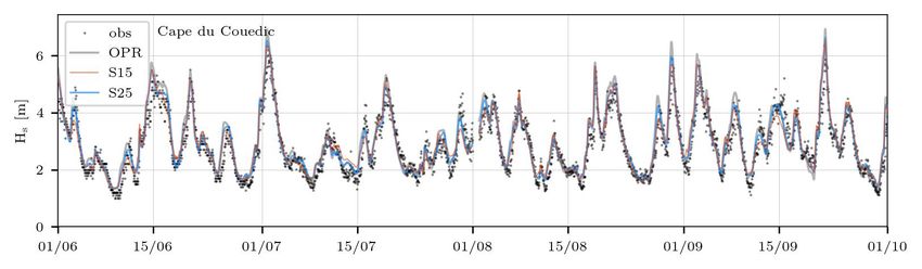
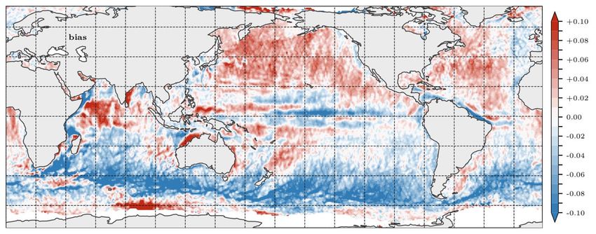
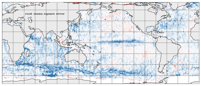
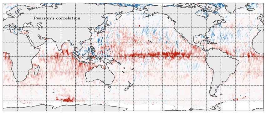
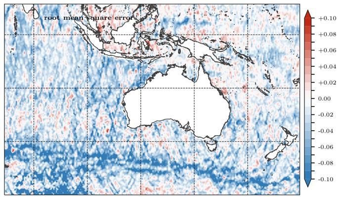
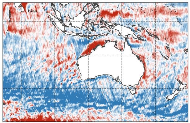
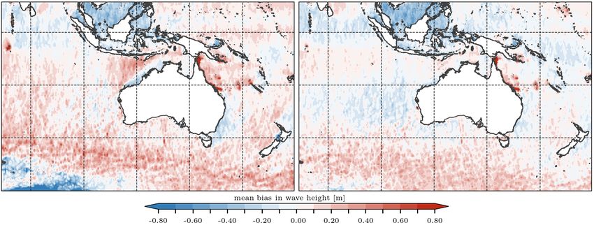
A MULTIPLE-RESOLUTION GLOBAL WAVE MODEL – AUSWAVE-G3

LIST OF FIGURES

Figure 1 Wave spectra (top panels) and nonlinear four-wave interaction term (bottom
 panels) relative to peak wave frequency. Results are shown for the duration-limited test
 after 36 h for unidirectional winds (left) and turning winds (right). This test is WW3
 regression test ww3_ts1 with ST6 source term (WW3DG 2019). ........................................... 8
Figure 2 Location of Australian wave buoys used for model evaluation (for label names see
 Table 1). Solid blue shading represents areas of less than 75m depth. .............................. 10
Figure 3 Depths from the two gridded bathymetries compared to measured water depths
 at the 45 buoys listed in Table 1. Buoy ID references to the first column of Table 1. The
 dashed line shows the 75 m depth contour. .................................................................................. 13
Figure 4 Map of SMC grid around Australia. Shading shows grid resolutions with 1/8° x 1/8°
 (pale blue) and 1/16° x 1/16° (purple). .......................................................................................... 14
Figure 5 Map of SMC grid cell sizes at high latitudes. Shading shows four grid resolutions:
 1/8° (pale blue) and 1/16° (purple) up to 55° latitude; 1/8°x1/4° between 55° and 70°
 latitude (blue) and 1/8°x1/2° beyond 70° latitude (dark blue). ........................................... 15
Figure 6 Taylor diagram showing model skill for sea surface wind speed for ACCESS-G3 over
 the global (G) and regional (R) domains. A superior model is closer to the triangle
 (observations) and to 1.00 arc normalized standard deviation. The asterisk represents
 a reference value for ACCESS-G1 winds (Durrant & Greenslade 2010). ............................ 17
Figure 7 Scatter comparisons for ACCESS-G3 surface wind speed (global). Top panels:
 radiometer winds (AMSR2); bottom panels: scatterometer winds (ASCAT). Refer to
 Table 3 for statistic labels. ..................................................................................................................... 17
Figure 8 Spatial distribution of wind speed bias (B) relative to (top panel) radiometer winds
 and (bottom panel) scatterometer winds. ...................................................................................... 18
Figure 9 Spatial distribution root-mean-square error (E) for surface wind speed relative to
 (top panel) radiometers and (bottom panel) scatterometers. ............................................... 19
Figure 10 Taylor diagram showing the model skill for significant wave height for (left panel)
 global domain and (right panel) regional domain. The asterisks represent a reference
 value for AUSWAVE-G1 (Durrant and Greenslade 2010). OPR refers to current
 operational configuration forced with ACCESS-G3 winds. ...................................................... 25
Figure 11 Scatter comparison for selected wave model configurations (see Table 5).
 Statistics are based on altimeter data for the global domain. Top panels represent
 operational model (OPR); middle panels to S15; bottom panels to S25. ........................... 25
Figure 12 Spatial distribution of mean bias for altimeter for configuration OPR (top
 panel), S15 (middle panels) and S25 (bottom panel). ............................................................... 26
Figure 13 Spatial bias for significant wave height for AUSWAVE-R domain for configuration
 OPR (left panel) S15 (right panel). ..................................................................................................... 28
Figure 14 Taylor diagrams showing the model skill for significant wave height (Hs). The
 asterisks represent a reference value for operational configuration (OPR). Wave buoy
 observations were sourced from moored and drifitng buoys (see Table 1). ................... 30
Figure 15 Spatial distribution of mean bias in altimeter for AUSWAVE-R domain. Panels
 show non-current simulation S18 (left) and an ocean current simulation S15 (right).
 ........................................................................................................................................................................... 31
Figure 16 Spatial distribution of mean bias for altimeter for ocean current simulation
 S18 (top panel) and a non-current simulation S15 (bottom panel). ................................... 32

iv
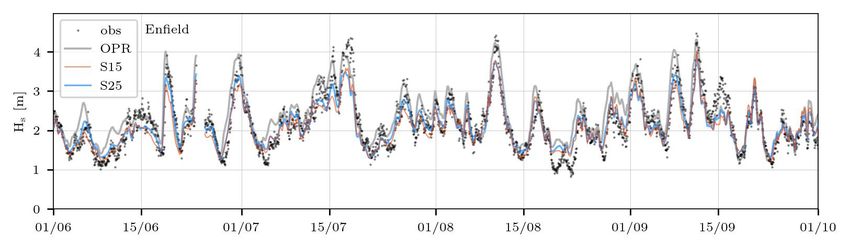
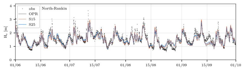
A MULTIPLE-RESOLUTION WAVE MODEL – AUSWAVE-G3

Figure 17 Bottom panel: Changes in root-mean-square error (E; units: m) for altimeter
 in the Australian domain. Changes were calculated between a current simulation (S15)
 and a simulation without ocean currents (S18). Top panel: differences between the two
 fields. A positive value means an increase in ocean current simulation relative to the
 non-current simulation. .......................................................................................................................... 33
Figure 18 Changes in verification metrics for altimeter between a simulation with ocean
 currents (S15) and without currents (S18). Top panel show the differences between the
 two fields. Verification metrics include: root-mean-square error (E; units: m) and
 correlation coefficient (R; dimensionless). A positive value means an increase in a
 metric in S15 relative to S18 model configuration. ..................................................................... 34
Figure 19 Schedule for AUSWAVE-G3 experimental forecast system showing four
 consecutive forecast cycles (forecast range: +7 days). .............................................................. 35
Figure 20 Model skill (vertical axis) for surface wind speed plotted as a function of lead time
 (horizontal axis; units: hours). Panels show selected verification metrics (from top):
 root-mean-square error (E; units: m s-1), Pierson’s correlation (R), scatter index (SI)
 and bias (B; units: m s-1). Line types indicate results from different domains.
 Observations are based on scatterometer data (ASCAT). ......................................................... 38
Figure 21 Model skill (vertical axis) for wave height ( ) plotted as a function of lead time
 (horizontal axis; units: hours). Panels show selected verification metrics (from top):
 root-mean-square error (E; units m), Pierson’s correlation (R), scatter index (SI) and
 bias (B; units: m). Line types indicate results from different model domains and models
 (i.e. operational model (grey), S15 configuration (orange)). Observations were
 compiled from satellite altimeters for global and regional domains and wave buoys for
 coastal verification. ................................................................................................................................... 39
Figure 22 Growth in wave height error (E; units: m) as a function of model lead time (units:
 hours). Plot shows global altimeter error for confirmation S15 and least-square
 regression (1st order and 2nd order) as function of wind speed error 10. .................... 41
Figure 23 Buoy and model time series for significant wave height (units: metres) for the
 entire hindcast period. Model results are shown for operational AUSWAVE-G3 interim
 (OPR) and configurations S15 and S25. See Table 1 and Figure 2 for wave buoy details.
 ........................................................................................................................................................................... 53
Figure 24 Buoy and model time series for peak wave period (units: seconds) for the entire
 hindcast period. Model results are shown for operational AUSWAVE-G3 interim (OPR)
 and configurations S15 and S25. See Table 1 and Figure 2 for wave buoy details. ..... 61
Figure 25 Buoy and model time series for peak wave from direction (units: degree) for the
 entire hindcast period. Model results are shown for operational AUSWAVE-G3 interim
 (OPR) and configurations S15 and S25............................................................................................. 68

v

A MULTIPLE-RESOLUTION WAVE MODEL – AUSWAVE-G3

ABSTRACT

A new wave forecast system has been developed with the objective of replacing the Bureau
of Meteorology’s global and national wave forecast models AUSWAVE-G and AUSWAVE-R.
The new wave model (AUSWAVE-G3) features ~12km spatial resolution globally with
refinement around sub-grid scale features at ~6km resolution and uses guidance from the
Bureau's numerical weather and ocean prediction systems ACCESS-G3 and OceanMAPS.
Including ocean currents in the wave model is the first step towards a coupled modelling
system, an objective of the Bureau's Research and Development Plan 2020–2030.
The model was calibrated over a 4-month hindcast period (June – September 2020) and
evaluated for forecast skill over a 3-month period (November 2020 – January 2021). Model
verification is based on observations from; satellite scatterometers and radiometers for
marine surface winds, and satellite altimeters and Australian wave buoys for ocean waves.
Verification metrics presented in tables and figures consistently show that the proposed
new AUSWAVE-G3 configuration outperforms the existing operational system for a large
number of verification metrics. The forecast error in significant wave height at +7 days
is nowadays similar to that of +4 days of AUSWAVE-G1 (2011). Altimeter verification shows
a root-mean-square error in of 0.31 m for the global model, which is an improvement of
~0.05 m (16%) compared to the existing operational wave model.
The new multi-resolution global wave model provides seamless wave forecasts up to +7
days at higher-resolution around Australia. This is an improvement over the existing
regional domain wave model AUSWAVE-R that is limited to forecasts range of +3 days.

1
A MULTIPLE-RESOLUTION GLOBAL WAVE MODEL – AUSWAVE-G3

1. INTRODUCTION

The Bureau of Meteorology (henceforth the Bureau) has an important role in providing
marine services around Australia and its surrounding oceans. These services have a strong
dependence on guidance from numerical wave models, which in turn are dependent on
numerical weather prediction (NWP) systems. At the Bureau, current NWP guidance is
based on the Australian Community Climate and Earth System Simulator (ACCESS; Puri et
al. 2013). Over the past decade the Bureau’s ACCESS systems have vastly improved their
skill as a result of progressing improvement of increase in horizontal and vertical
resolution, enhanced data assimilation (including increasing numbers and types of
observations) and improvements in physical parameterisations.
The most recent implementation of the Bureau’s ACCESS system (ACCESS-G3) is a global
data assimilating atmospheric model with a horizontal resolution of N1024, equivalent to
~12 km. This system became operational in July 2019 (NOC 2019). In addition to providing
surface wind forcing for the operational wave model, ACCESS provides surface stress and
heat fluxes for the operational ocean model OceanMAPS (Brassington et al. 2007; Huang et
al. 2020).
Following the NWP systems, operational wave models have shown large improvements in
skill over the past decade (e.g. Janssen & Bidlot 2018). At the Bureau, the resolution of the
wave model traditionally follows that of the underlying NWP system. With introduction of
ACCESS, the Bureau’s operational wave model AUSWAM (WAMDI 1988) was upgraded to
AUSWAVE which is an implementation of the WAVEWATCH III (WW3DG 2019) wave model
(Durrant & Greenslade 2011). The most recent operational version of AUSWAVE (NOC
2016a), is referred to here as AUSWAVE-G2 with the '2' referring to the wind forcing being
provided by ACCESS-G2. The 2019 upgrade to ACCESS-G3 meant that horizontal resolution
in the global wave model required improvement. Upgrading an operational wave model
comes with constraints and for the present upgrade to the Bureau’s marine forecast system,
has three key requirements: (i) a global resolution that approximately matches ACCESS-G3
(12 km), (ii) an increase in lead time from 7 days to 10 days, and (iii) a 2-hour time limit for
the model run-time. Upgrading AUSWAVE-G2 to AUSWAVE-G3 means doubling the
resolution. For reference a rectilinear wave model grid, the rule of thumb is that doubling
the resolution requires 8 to 10 times more compute resources (see column cost in Table 5).
The present work analyses state-of-the-art wave model physics and their potential for
retuning the Bureau’s global operational wave model, given the availability of new surface
forcing from ACCESS-G3. In addition, the benefit of providing ocean currents to the wave
model from the OceanMAPS system is investigated.
The paper is arranged as follows. Section 2 presents some basics of wave model physics and
relevant tuning parameters. Section 3 describes the observational datasets used for model
calibration and verification. Section 4 provides a description of various configuration
options for AUSWAVE-G3, such as the model grid and bathymetry dataset. It also includes a
verification of the surface forcing winds. Wave model calibration and forecast verification
are presented in sections 5 and 6, respectively. Discussion and conclusions are presented at
the end in sections 7 and 8.

2
A MULTIPLE-RESOLUTION WAVE MODEL – AUSWAVE-G3

2. GOVERNING EQUATIONS

WAVEWATCH III (WW3) is a dynamic numerical model to simulate the variance density
spectrum of surface gravity waves (henceforth referred to as the wave spectrum). It is a
third-generation wave model which means that the model explicitly accounts for the four-
wave resonant interactions in the source terms (see section 2.2). WW3 has seen a number
of improvements over the past decade and was recently upgraded to version 6.07 (WW3DG
2019). The model supports multiple grid types including regular, rotated, curvilinear,
unstructured, tri-polar, multi-resolution and Cartesian grids. The model framework also
features two-way nesting between different grid types. Originally developed as global wave
model the new version has improved support for coastal applications with variable
resolution unstructured grids (e.g. Abdolali et al. 2020). WW3 includes a range of wind input
and wave attenuation source terms. Stopa et al. (2016) showed that for stand-alone wave
model simulations with prescribed surface winds, ST4 and ST6 source term packages (see
section 2.1) produced the highest quality wave fields and spectral parameters (see also
Zieger et al. 2015, 2021).
Third-generation wave models operate under the assumption that the wave field is
homogenous and slowly varying in time. Growth and decay of the wave spectrum is based
on fluxes and physical processes related to wind-wave processes represented by source
terms. These source terms are all parameterised as functions of the wave spectrum. The
wave spectrum is five-dimensional ( , , , ) and is a function of wavenumber , wave
direction , time , and two-dimensional space . To discretise the five-dimensional wave
spectrum ( , , , ), two types of resolution are used: (i) spectral resolution ( by
elements) and (ii) spatial resolution ( 1 by 2 elements that define two-dimensional
space ). Integrating the wave spectrum yields an estimate for significant wave height :
 1/2
 = 4 [ ∬ ( , ) ] .

High spatial resolution is important for wave propagation in regions with small islands and
atolls (e.g. the South Pacific, Great Barrier Reef and the Indonesian Archipelago) while high
spectral resolution is important for the depiction of the propagation of swell fields across
large distances to avoid an effect known as the garden sprinkler effect (Booij & Holthuijsen
1987). For example for waves under intense and constantly changing winds (i.e. tropical
cyclones). The garden sprinkler effect can be mitigated by increasing the number of
directions and/or frequency increments in wave spectra, however this significantly
increases the number of equations in the wave model (see next paragraph). Wavenumber
and intrinsic frequency satisfy the dispersion relation 2 = tanh( ) where is the
gravitational constant and is mean water depth. Under a slowly varying current a Doppler
shift is applied to the intrinsic frequency .
The governing equation for the evolution and propagation of wind-waves can be written as
(Gelci et al. 1957)

 + ∇ ̇ + ̇ + ̇ =
 ∂t ∂k ∂θ
The terms on the left-hand side represent the rate of net change of wave spectral densities
and the advection of wave spectral densities. Spectral advection is ̇ = / in geographic

3
A MULTIPLE-RESOLUTION GLOBAL WAVE MODEL – AUSWAVE-G3

space, ̇ = / in wavenumber space and ̇ = / in direction space. This means that
a total of 1 ∙ 2 ∙ ∙ equations is solved by the model at each time step.
The right-hand side of the governing equation is the total source term which describes
all known physical processes in the form of spectral functions. In deep water, the dominant
processes are wind input , four-wave resonant interactions and wave dissipation .
Wave dissipation includes three different types of dissipation: wave breaking, white-
capping and non-breaking dissipation. Wave breaking and white-capping dissipation are
parameterised in the term. In shallow water additional processes such as depth limited
breaking ( ) and bottom scattering ( ) need to be accounted for.
 = + + + +
The wind input, resonant four-wave interaction, and dissipation source terms are
considered the primary source terms and the mechanisms behind fetch-limited and
duration-limited wave growth (Hasselmann 1960). Their purpose is the generation of
waves, transfer of energy between waves, and removal of energy from the spectrum. Across
large ocean basins, dissipation of non-breaking swell waves (hereafter swell dissipation)
becomes increasingly important. Retuning of some aspects of the wind input and
dissipation source terms should be handled with care, because the source terms have been
developed to provide a balance for wave growth and decay under the assumption that the
forcing wind field is free of errors. Any retuning thus largely compensates for errors in the
wind field but through a highly non-linear system of differential equations. This effectively
leaves three options for model tuning in deep water: (i) adjusting wind scaling parameters,
(ii) adjusting swell dissipation coefficients, and (iii) adjusting non-linear four-wave
interaction coefficients.

2.1 Wind-input and swell dissipation terms

In spectral wave models, all source terms are parameterised as a function of the directional
wave spectrum ( , ). As mentioned earlier, the wind input terms are responsible for the
generation of waves. Swell dissipation is non-breaking wave dissipation due to turbulence
in the wave-boundary layer on either side of the air-sea interface. This can either be
represented as part of the wind input term for the atmospheric side, or for the ocean side,
as a separate dissipation term. The generic form of the wind input term is written as

 ( , ) = ( , ) ( , )

where , are densities of air and water, = 2 is the intrinsic radian frequency of
wave components and ( , ) is the wave growth rate. For a WAM cycle 4 type wind input
(Janssen 1991) such as ST4, the growth rate is given as
 ∗ 2
 ( , ) = −1 exp( ) 4 ( + ) cos 2( − )

where is a non-dimensional scaling parameter, is the von Kármán’s constant, is
the effective wave age, is the phase speed of spectral wave components, is a wave age
tuning parameter, and ∗ is the wind stress relative to wave direction ( − ). Effective

4
A MULTIPLE-RESOLUTION WAVE MODEL – AUSWAVE-G3

wave age Z is a set of functions of roughness length 0 , phase speed , wave supported stress
 ∗ and wind stress relative to wave direction (Janssen 1991).

 = log( 0 ) +
 cos ( − )( ∗ ⁄ + )
For the ST6 wind input, the growth rate is given as (Zieger et al. 2015)
 ( , ) = ( , ) √ ( ) ( , )
 ( , ) = 2.8 − [1 + tanh ( 10 √ ( ) ( , ) − 11)]
 2
 ( , ) = [ cos( − ) − 1]

where ( ) is spectral saturation and = 32 ∗ is the wind speed1 relative to wave
direction.
Adjustment of fluxes has generally been the principal method to calibrate a wave model.
Increasing the appropriate coefficient effectively translates to an increase in momentum
flux and yields stronger wave growth. In the case of ST4 this can be done with the non-
dimensional scaling parameter (BETAMAX in Table 4 and Table 5). With the ST6
source terms (Zieger et al. 2015) an equivalent scaling was implemented through an
extension of the flux parameterisation (Hwang 2011). The extension added a simple scaling
parameter (CDFAC in Table 4 and Table 5) to estimate surface drag coefficient to
convert from 10 m surface winds 10 to wind stress ∗ :
 2
 ∗2 = 10 ( ∙ s)
In relation to swell dissipation tuning, empirical guidance on the swell dissipation
coefficient exists (Ardhuin et al. 2009, Young et al. 2013), however the magnitude of those
coefficients is too high when incorporated into a global wave model suggesting that it is not
constant (Zieger et al. 2015). The ST4 swell dissipation term is added to the wind
input term . The swell dissipation coefficient of the turbulent part of the swell term is
based on Grant-Madsen friction value , and Taylor expansion as a function of wind and
wave direction and the ratio of wind stress to wave orbital velocity (Ardhuin et al.
2010).

 ( , ) = − 16 2 −1 ( , )

 = 1 { , + [| 3 | + 2 cos( − )] ∗ }

On the other hand, ST6 source terms have two coefficients for swell dissipation. One is
included in the growth rate of the wind input term to accommodate turbulence in the
atmosphere ( 0 ; SINA0 in Table 4).
 ( , ) = 1 ( , ) − 0 2 ( , )
 2
 1 = max [ cos( − ) − 1 , 0]
 2
 2 = min [ cos( − ) − 1 , 0]

1Friction velocity scaling is a tuneable parameter in the ST6 wind input term (Liu et al. 2019). If changed, the dissipation term
 for wave breaking and whitecapping would have to be recalibrated.

5
A MULTIPLE-RESOLUTION GLOBAL WAVE MODEL – AUSWAVE-G3
The second one is a dedicated swell dissipation term and accommodates turbulence in the
ocean ( 1 ). Compared to wave breaking and whitecapping dissipation , swell
dissipation is orders of magnitude lower (Zieger et al. 2015).
2
( , ) = √ ( ) ( , )
3 1
2.2 Four-wave resonant interaction source term
The wind input and dissipation terms operate locally in spectral space and therefore can
increase or decrease the amplitude of individual spectral components. The four-wave
resonant interaction term is different and is responsible for the redistribution between the
amplitudes of individual components in spectral space (Hasselmann 1962). It plays a critical
role in reproducing the observed down-shift of spectral densities towards lower
frequencies during wave development. The redistribution takes place between four
different wave components that satisfy the resonance conditions
1 + 2 = 3 + 4 ,
1 + 2 = 3 + 4 .
The Boltzmann integral describes the exact solution that satisfies the resonance condition
for two interactions in a five-dimensional phase space. Hasselmann et al. (1985) compared
a couple of options for nonlinear interaction source terms and forged the idea that that the
principal features of the nonlinear transfer of spectral components can be considered as
superposition of a small number of discrete-interaction approximations (DIA). Each
configuration is identical to the computation of the exact solution of the Boltzmann integral,
except that it is solved for two interactions in two-dimensions in phase space. Similar to the
solution of the full Boltzmann integral, the DIA conserves energy, momentum and action.
For a JONSWAP type spectrum Hasselmann et al. (1985) found good agreement with the
exact solution when using one single configuration with = 0.250 (LAMBDA in Table 4 and
Table 5) being a free shape parameter and
1 = 2 =
{ 3 = (1 + ) = +
4 = (1 − ) = −
For wavenumbers 3 ( + ) and 4 ( − ) the resonant condition utilizes constant angles
relative to , which are 3 = 11.5° for 3 , 4 = −33.6° for 4 . The nonlinear interaction
source term (DIA) as a function of the wave spectrum ( , ) can be written as
Δ Δφ
−2 Δ Δφ
+ Δ Δ + − + −
{ } = (1 + )Δ +Δ × −4 11 [ 2 ((1+ ) 4 +(1− )4 ) − 2(1− 2 )4 ]
−
Δ Δ
{(1 − )Δ −Δ }
where is a proportionality coefficient and Δ , Δ + , Δ − represent discrete resolution of
the spectrum at frequencies , + , −. The proportionality coefficient C was empirically
determined by model tuning and was later extended to allow scaling that accounts for the
6A MULTIPLE-RESOLUTION WAVE MODEL – AUSWAVE-G3
effects of shallow water (Hasselmann & Hasselmann 1985). The original value of coefficient
(NLPROP in Table 4 and Table 5) was determined for the WAM wave model as 3 × 10⁷ ,
which leaves room for some retuning for the DIA in WW3. Hasselmann et al. (1985)
acknowledged that the DIA reproduced the positive lobe of the spectrum, however the
redistribution of spectral densities at high frequencies showed large errors. Nonetheless,
the positive lobe controls the downshift of the spectral peak towards lower frequencies and
that resulted in satisfactory correspondence with empirical growth curves. Acknowledging
the shortcomings of the DIA, Tolman (2013) added a nonlinear source term to allow the
computation of the Boltzmann integral for multiple DIA configurations (see NQDEF and
QPARMS in Table 4 and Table 5). Tolman & Grumbine (2013) provide guidance on how to
retune a set of multiple DIA configurations. Multiple DIA configurations include two new
shape parameters and . The latter is the angle between wavenumber vectors 1 and 2
(Tolman 2013). Setting shape parameters = 0 and = 0 is equivalent to the Hasselmann
et al. (1985) configuration. Multiple DIA configurations (QPARMS in Table 5) are given as
1−
2 =
1+ 1
1+
3 =
1+ 1
1−
4 =
1+ 1
1 ∙ 2
12 = arccos
{ 1 2
Figure 1 shows the differences in spectral shape for a set of configurations based on a
duration-limited test with constant wind speed of 12 m s-1 (left panels) and turning winds
(right panel) for ST6 source terms (i.e. wind input and dissipation). Configurations plotted
in this figure correspond to three different options for the DIA and one using the exact
solution of the Boltzmann integral. The bottom panels show the redistribution of wave
components by relative to the peak frequency. Increasing the number of quadruplets
(GMD 5) comes close to the exact solution as illustrated in the right panels in Figure 1.
However, increasing the number of quadruplets comes at the cost of increased computation
time: for 5 quadruplets, this is roughly 1.6 times that of the DIA in case of a global hindcast
(see Table 5). An increase in run time makes a five-quadruplet configuration unsuitable for
global applications such as AUSWAVE-G3. However, for some applications, such as regional
scale tropical cyclones, a more accurate term is feasible. For example, Zieger et al. (2021)
demonstrated excellent skill across a large number of historical tropical cyclone cases with
no significant increase in runtime.
7A MULTIPLE-RESOLUTION GLOBAL WAVE MODEL – AUSWAVE-G3 Figure 1 Wave spectra (top panels) and nonlinear four-wave interaction term (bottom panels) relative to peak wave frequency. Results are shown for the duration-limited test after 36 h for unidirectional winds (left) and turning winds (right). This test is WW3 regression test ww3_ts1 with ST6 source term (WW3DG 2019). 8
A MULTIPLE-RESOLUTION WAVE MODEL – AUSWAVE-G3

3. OBSERVATIONS

In the following sections, we undertake various calibration and verification exercises. These
include: evaluation of two possible bathymetry datasets; verification of the ACCESS-G3
wind fields; calibration of the AUSWAVE-G3 wave model; and verification of the wave model
forecasts. Observations used for the verification analyses have been obtained from a variety
of sources. Details of these observational reference datasets are outlined in this section.

3.1 Satellites

Surface wind data was sourced from Remote Sensing Systems online archive2. The online
archive provides global daily fields of marine surface wind speed (at 10 m above the
surface) from a number of different platforms and sensors. We used passively sensed
radiometers (AMSR2) and actively sensed scatterometer (ASCAT) winds. No additional
quality control was applied to wind speed observations. Note that these instruments
observe properties of the ocean surface (i.e. roughness length and brightness temperature)
and therefore indirectly measure wind speed. Radiometers tend to have a fair-weather bias
and drop out in the presence of moderate rain. Zieger et al. (2014) identified differences of
up to 0.8 m s-1 between altimeter and radiometer derived winds depending on latitude.
Young & Donelan (2018) also identified systematic differences in radiometer wind speeds
that not only varied with latitude but also with season and attributed these differences to
changes in atmospheric stability and the shape of the boundary layer. This note is relevant
for the assessment of wind speed error in section 4.4. Observational error for radiometer
wind speed is stated as 0.9 m s-1 for the no-rain condition relative to in-situ buoy
observations (Zieger et al. 2014; Young et al. 2017). The error for scatterometer winds
(ASCAT) is stated as 0.98 m s-1 (Ribal & Young 2020).
Remotely-sensed wave data was sourced from the altimeter database (RADS). Satellite
altimeters actively sense along a regularly repeated ground track and have nearly global
coverage (polar regions are missing). Here we used data from Sentibal-3a, b, Cryosat-2, and
Jason-2, 3 altimeter missions. Altimeter data was quality controlled based on the quality
flags and calibrated using the correction functions of Ribal & Young (2019).
Quality controlled and calibrated altimeter data is expected to have an error of less than
0.25m for (Zieger et al. 2009).

3.2 Wave buoys

Wave data from in situ buoys was primarily sourced from the Australian Ocean Data
Network3. Data at a small number of sites (5) was sourced from our industry partners (e.g.
Oceanum, Woodside, and Chevron). Wave data includes the integral parameters: significant
wave height, peak wave period and peak wave direction. Note that peak wave period and
peak wave direction were less frequently provided in the dataset. Visual quality control was
applied to check for gross errors in the dataset. Wave buoys are considered ground truth

2 www.remss.com
3 https://portal.aodn.org.au

9
A MULTIPLE-RESOLUTION GLOBAL WAVE MODEL – AUSWAVE-G3

and therefore no calibration was applied. Error in is stated as 0.5% of the observed value
for Datawell Buoys4. In addition, measured water depth at these buoy locations (and several
other historical buoy locations where wave data was not available) was used for evaluation
of bathymetry data.
Table 1 lists details of all buoys used, either for wave calibration/verification or for
bathymetry evaluation. Figure 2 show the locations of the wave buoys used for calibration
and verification.

Figure 2 Location of Australian wave buoys used for model evaluation (for label names see Table 1). Solid blue
shading represents areas of less than 75m depth.

4 https://www.datawell.nl/Products/Buoys.aspx

10
A MULTIPLE-RESOLUTION WAVE MODEL – AUSWAVE-G3

Table 1 List of Australian wave buoys used for model evaluation sorted according to recorded depth. IDs and
names formatted bold were used for model verification and are indicated in Figure 2. Note that Sowb1 is a
drifting buoy.
 ID Name Latitude (°S) Longitude (°E) Measured depth (m) DBDB2 GEBCO
 (m) (m)
 1 Albatross Bay 12.68 141.68 10 17 20
 2 Hay Point 21.27 149.31 10 11 26
 3 Ashburton 21.54 115.03 11 21 18
 4 Caloundra 26.85 153.16 12 38 28
 5 Skardon River offshore 11.75 141.92 12 23 10
 6 Gladstone 23.90 151.50 13 30 26
 7 Abbot Point 19.87 148.10 14 30 30
 8 Cairns 16.73 145.72 15 27 28
 9 Dampier 20.44 116.73 15 59 24
 10 Port Hedland 20.01 118.44 17 39 32
 11 Cottesloe 31.98 115.69 17 18 26
 12 Townsville 19.17 147.05 18 37 32
 13 Bundaberg 24.67 152.50 18 30 28
 14 Gold Coast 27.97 153.44 18 65 68
 15 Emu Park 23.30 151.07 22 7 44
 16 Skardon River outer 11.75 141.84 22 41 32
 17 Lakes Entrance 37.92 147.97 23 50 48
 18 Mackay 21.03 149.55 29 63 70
 19 Mandurah 32.45 115.57 30 36 52
 20 Point Nepean 38.36 144.69 30 102 72
 21 Mooloolaba 26.57 153.18 32 59 64
 22 Mackay Inner 21.10 149.26 34 28 22
 23 North Moreton 26.90 153.28 35 68 54
 24 Jurien Bay 30.29 114.91 42 89 68
 25 Wide Bay 25.80 153.17 43 79 84
 26 Rottnest Island 32.11 115.40 48 139 128
 27 Cape Naturaliste 33.36 114.78 50 94 136
 28 Esperance 34.00 121.90 52 109 112
 29 Lakes Entrance1 38.05 148.41 55 112 104
 30 Albany 35.20 117.17 60 140 142
 31 Tweed Offshore 28.21 153.68 60 122 124
 32 Byron Bay 28.87 153.69 62 124 118
 33 Batemans Bay 35.71 150.34 62 108 68
 34 Cape Bridgewater 38.36 141.27 69 162 174
 35 Wilsons Promontory 39.54 146.47 69 153 148
 36 Coffs Harbour 30.36 153.27 72 186 130
 37 Brisbane 27.50 153.63 73 104 136
 38 Kingfish B 38.60 148.19 78 154 150
 39 Crowdy Head 31.81 152.86 79 161 146
 40 Port Kembla 34.47 151.02 80 159 156
 41 Cape Du Couedic 36.07 136.62 80 175 146
 42 Sydney 33.77 151.41 92 200 206
 43 Eden 37.26 150.19 100 234 208
 44 Cape Sorell 42.08 145.01 100 214 202
 45 North Rankin 19.59 116.14 125 230 236
 46 Campbell Island 52.76 169.04 147 407 520
 47 Enfield 21.48 114.00 — — —
 48 Ichthys 13.91 123.26 — — —
 49 Prelude 13.82 123.29 — — —
 50 Goodrich Bank 10.42 130.00 — — —
 51 Sowb1 drifting drifting — — —

11
A MULTIPLE-RESOLUTION GLOBAL WAVE MODEL – AUSWAVE-G3

4. AUSWAVE-G3 CONFIGURATION

WW3 solves the governing equation for each component in the wave spectrum. As
described in section 2, the wave model is discretised in two types of resolution, that is
spectral resolution and spatial resolution. The previous implementation of AUSWAVE
featured a fixed spatial resolution (1/4° and 1/10°) across the entire domain. AUSWAVE-G3
uses a more complex spatial resolution that changes with latitude, depth and level of
subscale features (see section 4.2 for more detail). The local wave spectrum is resolved in
30 directional bins (i.e. 12° directional resolution) and 28 frequency bins with an increment
factor of 1.1 logarithmically spaced from 0.0412 to 0.5399 Hz.
WW3 model physics and parameterisations are selected by switches at compile time. In
addition to switches used for model calibration (see Table 4) the wave model was compiled
with depth induced breaking parameterisation (DB1) and bottom friction term (BT4) with
uniform medium sediment size 50 of 0.2 mm (WW3DG 2019). Compared to the empirical
linear JONSWAP bottom friction (BT1), BT4 scales with bottom wave orbital velocity,
orbital amplitude and Nikuradse roughness length and can lead to differences of 0.10 to
0.40m in significant wave height in shallow water (Zieger et al. 2018, 2021).
The wave model configuration includes a static bathymetry grid (see section 4.1) and
prescribed fields of spatially and temporally varying surface winds (see section 4.4), sea ice
concentration, and surface currents (see section 4.5). Sea ice is an auxiliary variable in the
ACCESS-G3 model suite that is based on NOAA/NCEP5 1/12° sea ice analysis (NOC 2019).

4.1 Bathymetry

The previous version of AUSWAVE used a bathymetry grid generated from the DBDB2
(version 3) bathymetry dataset. This was assessed to be the best bathymetry available at
the time of implementation (Durrant & Greenslade 2011). As part of the present upgrade,
and in the light of recent bathymetry dataset developments we evaluate here the GEBCO
2020 (GEBCO Bathymetric Compilation Group 2020) gridded bathymetry data against the
existing operational dataset.
The method used follows that of Durrant & Greenslade (2011) and Zieger et al. (2021).
Bathymetric depths for the two datasets are evaluated against measured depths derived
from wave buoy deployments around the Australian coastline. These are sourced from data
providers and are expected to be accurate to within approximately 1 m. The advantage of
using these measured depths is that firstly, they provide an independent source of
observations that have not been incorporated into the gridded bathymetries, and secondly,
they are directly relevant to the verification of wave model forecasts in the Australian
region. The buoys used are listed in Table 1. These are predominantly drawn from
Greenslade et al. (submitted to JOO) with the addition of the Campbell Island wave buoy
from New Zealand's Southern Ocean wave program (McComb et al., submitted to Scientific
Data).

5 National Oceanic and Atmospheric Administration/ National Centers for Environmental Prediction

12
A MULTIPLE-RESOLUTION WAVE MODEL – AUSWAVE-G3

For each buoy location, the depth at the closest point in each of the two bathymetries is
found. Results are shown in Figure 3. In general, both of the gridded bathymetries are
somewhat deeper than the measurements, with the difference increasing with depth. A
summary of the depth errors is shown in Table 2. Mean depth error and mean absolute
value of the depth error for the GEBCO 2020 bathymetry are marginally smaller than those
for DBDB2. When the comparisons are limited to buoys in water depth less than 75m (i.e.
depths which are more relevant for the propagation of wind waves) the improvement of
GEBCO 2020 over DBDB2 is more evident. These results suggest that there are benefits in
upgrading the operational bathymetry to GEBCO 2020.

Table 2 Summary of differences in measured depths and the two gridded bathymetries. B refers to bias, AE
refers to Absolute Error.
 Mean B Mean AE
 DBDB2 GEBCO 2020 DBDB2 GEBCO 2020
 All locations -52.2 m -50.9 m 53.1 m 51.5 m
 Locations less than 75m depth -36.4 m -33.8 m 37.5 m 34.6 m

Figure 3 Depths from the two gridded bathymetries compared to measured water depths at the 45 buoys listed
in Table 1. Buoy ID references to the first column of Table 1. The dashed line shows the 75 m depth contour.

13
A MULTIPLE-RESOLUTION GLOBAL WAVE MODEL – AUSWAVE-G3

4.2 Model grids

The AUSWAVE-G2 model grid was a regular spherical grid at 1/4° spatial resolution, limited
to 78°N and 78°S. One of the key issues with simply increasing the model resolution to
approximately match ACCESS-G3 is that the convergence of meridians reduces the actual
horizontal distance between grid points at high latitudes, which in turn requires a very
short propagation time step and a subsequent increase in computational run-time which is
not operationally feasible. Therefore, a number of alternative model grid configurations
were considered.
An initial model grid setup on the National Computational Infrastructure (NCI) followed
recommendations of Rogers & Linzell (2018), an approach based on the multi-grid model
consisting of one regular grid and two polar (curvilinear) grids with resolutions of 1/8° and
~12 km respectively (Zieger et al. 2019). Unfortunately, this irregular-regular-irregular
(IRI) model grid was not able to be ported to the Bureau's supercomputer due to a limit on
parallel communication channels in various versions of parallel libraries. This has been
noted in the WW3 documentation as a potential issue on some systems (WW3DG 2019). As
a result, this IRI grid was not pursued for AUSWAVE-G3.
As an alternative approach, the spherical multiple cell (SMC) grid (Li 2011) was selected
instead, with a base resolution of 1/8°, and an increase to 1/16° around islands and in
regions of less than 350 metres water depth. At high latitudes the grid relaxes in the
meridional direction to maintain a zonal resolution of ~12km. In other words, grid cells
change their aspect ratio at 55° (N and S) and 70° (N and S) to 1/8° (latitude) x 1/4°
(longitude) and 1/8° x 1/2° respectively. Grid refinement and relaxation is shown in Figure
4 for the oceans around Australia and Figure 5 for the Drake Passage between South
America and Antarctica.

Figure 4 Map of SMC grid around Australia. Shading shows grid resolutions with 1/8° x 1/8° (pale blue) and
1/16° x 1/16° (purple).

14
A MULTIPLE-RESOLUTION WAVE MODEL – AUSWAVE-G3

Figure 5 Map of SMC grid cell sizes at high latitudes. Shading shows four grid resolutions: 1/8° (pale blue) and
1/16° (purple) up to 55° latitude; 1/8°x1/4° between 55° and 70° latitude (blue) and 1/8°x1/2° beyond 70°
latitude (dark blue).

4.3 Output grids

Wave model field output for the SMC grid is in the form of a vector of sea points, equivalent
to an unstructured grid. In a post-processing step, these vectors are interpolated to a regular
latitude-longitude grid with a base resolution of 1/8° for the global grid (G08) and 1/16° for
a regional grid (R16), similar to the former AUSWAVE-R grid. The AUSWAVE-R domain covers
69°E–180°E and 60°S–12°N and is used for selected Bureau’s marine forecast services. All
interpolation is done by means of nearest-neighbour (kd-tree search algorithm).
Subsequent model verification is based on the interpolated output grids.

4.4 Surface winds

Stand-alone wave model simulations require fields from atmospheric models which means
that wave model accuracy is a function of the accuracy of the surface wind field. Errors in
wind fields can vary in space and time which makes it difficult to separate errors due to the
forcing from internal wave model errors. These can arise, for example from insufficient
model resolution, numerical schemes, and source term parameterisations. Errors in wind
sea can be mitigated in a fully coupled system, where the feedback from waves and ocean
to the atmosphere can address some of the error in the wind field (e.g. Janssen & Bidlot
2018; Wiese et al. 2020). Under the situation of a prescribed wind field such feedback is
missing.
In this section we undertake verification of the Bureau's ACCESS-G3 marine surface winds.
Since the accuracy of the wave model depends to first order on the quality of the surface
wind field, knowledge of the skill of the surface winds can provide a quasi "upper bound" to
the wave model skill. Tuning flux parameterisation in the wave model can to some extend
address some of the shortcomings in the wind field. The ACCESS-G3 model is run four times
a day and consists of two +10 day lead time cycles and two +6 day lead time cycles.

15
A MULTIPLE-RESOLUTION GLOBAL WAVE MODEL – AUSWAVE-G3

 A series of wave hindcasts was trialled for model tuning (see calibration in section 5). This
 hindcast covers a period of four months (01/06/2020 to 01/10/2020). The hindcast is
 forced with ACCESS-G3 surface winds (at a spatial resolution of ~12 km) compiled as a
 series of recurring 12-hour forecasts (hours 0-11) sourced from the Bureau’s operational
 archive.
 We verified these surface winds against satellite winds from scatterometers (ASCAT) and
 radiometers (AMSR) (see section 3). We use standard verification metrics as defined in
 Appendix A (page 47). Figure 6 shows a Taylor diagram providing a summary of the skill of
 the ACCESS-G3 surface winds. Compared to ACCESS-G1 (from Durrant & Greenslade 2010),
 the skill has improved significantly although it should be noted that the ACCESS-G1
 verifications were undertaken over a different time period. It can also be seen that the
 overall skill of ACCESS-G3 in the Australian region is slightly better than the skill over the
 globe (Figure 6) and the model skill when compared to scatterometers is slightly better than
 when compared to radiometers.
 As one would expect there is little difference in bulk statistics (see Table 3) between
 scatterometer and radiometer comparisons. The main difference between the two satellite
 products is a shift in the probability density plot over the range 5 – 10 m s-1 (Figure 7). In
 addition, from Table 3 it can be seen that over the global domain, the bias against
 radiometers is smaller (less negative) than against scatterometers. This difference can be
 seen in the spatial distribution of biases plotted in Figure 8. There is a positive model bias
 in the northern hemisphere and along continental shelves which partially cancels out the
 negative biases in the southern hemisphere, thus providing a smaller bias overall, but not
 necessarily reflecting better model skill. As explained in section 3.1, radiometer wind speed
 estimates can vary at high latitudes and between seasons. When considering root-mean-
 square error the spatial differences between scatterometer and radiometer comparisons
 are smaller (see Figure 9).
 The overall error (E) at 1.21–1.29 m s-1 is small and close to the observational error (see
 section 3.1) for both products. The slight negative bias overall suggests that there may be
 benefits in increasing the non-dimensional growth coefficients for tuning. Absolute error
 metrics (E, AE, B) are slightly better over the global domain, whereas normalized errors (R,
 SI, NE) are slightly better over regional domain. This could be explained with wind speed in
 the regional domain being slightly more energetic than in the global domain (final column
 Table 3).

 Table 3 Satellite verification statistics for ACCESS-G3 surface wind speed (units: m s-1). Statistics are shown for
 global (G08) and Australian domain (R16). Verification statistics include: number of points (N), root-mean-
 square error (E), mean-absolute error (AE), bias (B), correlation coefficient (R), histogram fit (I), scatter index
 (SI), normalised error (NE), slope (FIT0), standard deviations of model STD(M) and observations STD(O) and
 mean observation MEAN(O). See appendix for metric definitions.
 REG. N E AE B R I SI NE FIT0 STD(M) STD(O) MEAN(O)
ASCAT G08 65,126,843 1.21 0.87 -0.23 0.950 0.945 0.15 0.136 0.964 3.73 3.81 8.06
AMSR G08 79,625,773 1.26 0.93 -0.11 0.946 0.950 0.16 0.143 0.972 3.75 3.88 7.94
ASCAT R16 12,424,710 1.26 0.89 -0.34 0.955 0.944 0.14 0.131 0.960 4.05 4.06 8.71
AMSR R16 16,257,664 1.29 0.95 -0.23 0.952 0.944 0.15 0.134 0.968 4.09 4.14 8.71

 16
A MULTIPLE-RESOLUTION WAVE MODEL – AUSWAVE-G3

In general, the scatter density plots in Figure 7 and verification statistics show very high
correlation between model and satellite data. The model tends to underestimate extreme
conditions from about the 99-th percentile, a feature shared between both radiometers and
scatterometers. These verifications suggest that the root-mean-square error (E) of surface
wind speed from ACCESS-G3 is less than 1.3 m s-1 which includes a small negative bias of
~0.2 m s-1. Given the mean observed wind speed of approximately 8.0 m s-1 during this time
period, these are excellent results.

Figure 6 Taylor diagram showing model skill for sea surface wind speed for ACCESS-G3 over the global (G) and
regional (R) domains. A superior model is closer to the triangle (observations) and to 1.00 arc normalized
standard deviation. The asterisk represents a reference value for ACCESS-G1 winds (Durrant & Greenslade
2010).

Figure 7 Scatter comparisons for ACCESS-G3 surface wind speed (global). Top panels: radiometer winds
(AMSR2); bottom panels: scatterometer winds (ASCAT). Refer to Table 3 for statistic labels.

17
A MULTIPLE-RESOLUTION GLOBAL WAVE MODEL – AUSWAVE-G3

Figure 8 Spatial distribution of wind speed bias (B) relative to (top panel) radiometer winds and (bottom panel)
scatterometer winds.

18
A MULTIPLE-RESOLUTION WAVE MODEL – AUSWAVE-G3

Figure 9 Spatial distribution root-mean-square error (E) for surface wind speed relative to (top panel)
radiometers and (bottom panel) scatterometers.

4.5 Ocean surface currents

Ocean currents can interact with the surface wave field in multiple ways: (i) change the
wave direction, (ii) change the wave steepness, and (iii) change the surface roughness
length (Rapizo et al. 2018). Roughness length 0 is sea state dependent and of order 0.01 to
0.1mm. It acts in a similar manner to wall friction and can modulate the wind stress that can
lead to an increase or decrease in the flow in the lowest layers of the atmosphere (Wiese et
al. 2020).
Prescribing a slowly varying current field means that there is a need to account for the
frequency Doppler shift in the governing equation. Currents can also affect the group
velocity of the wave field and thus accelerate or decelerate spatial advection. Lastly, a
spatial gradient in the current field can change the wavenumber (magnitude and direction)
and this can result in additional wave refraction and dispersion. Wave-current interactions
based on linear theory can be included in the governing equation (Rapizo et al. 2018).

19
A MULTIPLE-RESOLUTION GLOBAL WAVE MODEL – AUSWAVE-G3

Hersbach & Bidlot (2008) investigated the effect of ocean currents on the wave field using
the ECMWF’s coupled atmosphere-wave-ocean model and formulated a solution for relative
wind speed
 ⃗ in a moving frame of reference. The relative flow
 ⃗ can be expressed as

 ⃗ =
 ⃗ 10 −
 ⃗
where ⃗ is the surface current vector and is a reduction factor (see RWNDC in Table 4
and Table 5). Note that a relative wind speed will account for a fraction of the error in
the wave field. Bidlot (2010) noted that prescribing surface currents resulted in small
adjustments in the wind profile and thus the surface stress which had an effect on local wave
growth. Hersbach & Bidlot (2018) noted that absolute wind speed (at 10 m) above an ocean
current is expected to increase in the direction of the current due to reduced friction at the
surface and slightly decrease if opposed to the current. A follow-up study showed that the
effect of ocean currents is smaller than initially assumed and the reduction factor is
considered to be about half ( = 0.5; Bidlot 2012).
It has been demonstrated that by including currents in the wave model, one can address
biases in significant wave height in the Southern Ocean (Rapizo et al. 2018) and globally
(Bidlot 2010, 2012; Echevarria et al. 2019). These studies conclude that the benefit largely
comes from changes to the relative wind speed ⃗ . Any effects from additional refraction
of the wave field due to currents was found to be less dominant and largely depends on
whether the ocean model is able to resolve eddies. Using a theoretical eddy simulation,
Rapizo et al. (2018) noted that refraction errors in the ocean models increase if the spatial
resolution is coarser than 1/10°. In a follow-on study, Echevarria et al. (2019) was able to
show an improvement in wave direction in the Indian Ocean for Southern Ocean swell.
The Bureau has been running the global ocean circulation model Ocean Model Analysis
Prediction System (OceanMAPS) operationally since 2007. It has undergone several
upgrades over the years, and the latest implementation (version 3.3) is 'eddy-permitting'
with a horizontal resolution of 1/10° and 51 vertical levels. It incorporates an Ensemble
Kalman Filter data assimilation scheme and ingests in-situ profiles of temperature and
salinity, altimeter sea-level observations and sea surface temperature data from various
satellites. The ocean model generates +7 day forecasts and is scheduled to run once a day
(Huang et al., 2020). Aijaz el al. (2020) evaluated the skill and performance of OceanMAPS.
They found an annual mean absolute error (AE) of 0.11 m s-1 and a correlation of 0.71 for
surface currents. In Section 5, we trial some wave model configurations in which the ocean
currents from OceanMAPS are provided as a prescribed field to WW3. The 4-month hindcast
time series is compiled as a recurring series of 24-hour forecasts (hours 0-23).

20
You can also read