Design, Modelling and Control of a Space UAV for Mars Exploration - Akash Patel Space Engineering, master's level (120 credits)
←
→
Page content transcription
If your browser does not render page correctly, please read the page content below
Design, Modelling and Control of a Space
        UAV for Mars Exploration

                              Akash Patel

         Space Engineering, master's level (120 credits)
                             2021

                       Luleå University of Technology
        Department of Computer Science, Electrical and Space Engineering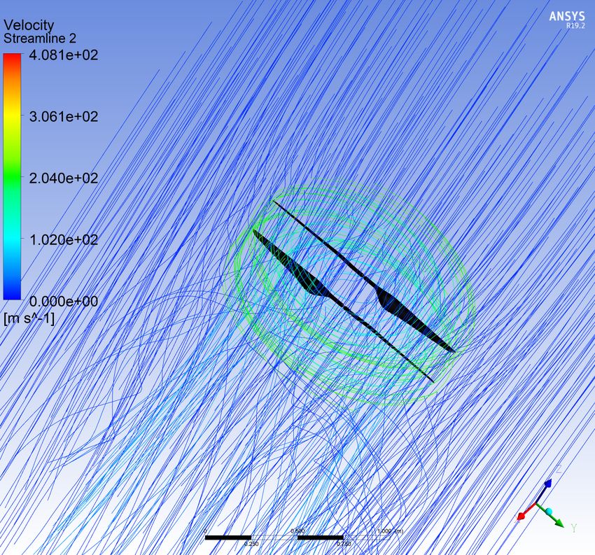
Design, Modelling and Control of a Space UAV for
               Mars Exploration

                                   Akash Patel

         Department of Computer Science, Electrical and Space Engineering
                     Faculty of Space Science and Technology
                           Luleå University of Technology

             Submitted in partial satisfaction of the requirements for the
                                   Degree of Masters
                          in Space Science and Technology

                      Supervisor     Dr George Nikolakopoulos

                                     January 2021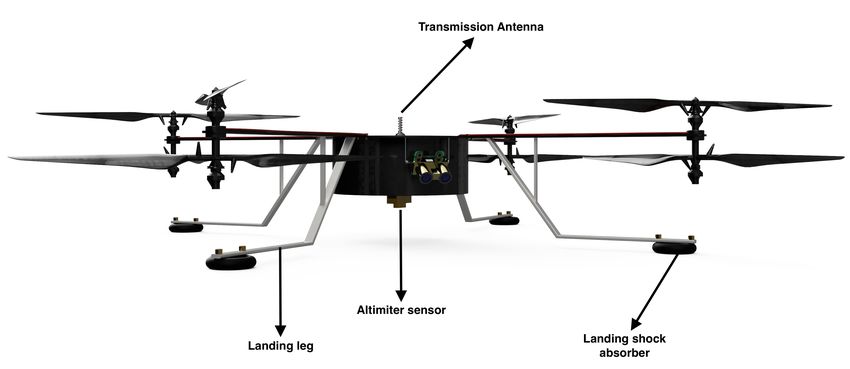
Acknowledgements

I would like to take this opportunity to thank my thesis supervisor Dr. George Nikolakopoulos who
has laid a concrete foundation for me to learn and apply the concepts of robotics and automation
for this project. I would be forever grateful to George Nikolakopoulos for believing in me and for
supporting me in making this master thesis a success through tough times. I am thankful to him
for putting me in loop with different personnel from the robotics group of LTU to get guidance on
various topics. I would like to thank Christoforos Kanellakis for guiding me in the control part of
this thesis. I would also like to thank Björn Lindquist for providing me with additional research
material and for explaining low level and high level controllers for UAV. I am grateful to have been
a part of the robotics group at Luleå University of Technology and I thank the members of the
robotics group for their time, support and considerations for my master thesis.

I would also like to thank Professor Lars-Göran Westerberg from LTU for his guidance in develop-
ment of fluid simulations for this master thesis project. I would like to express my gratitude towards
Dr Victoria Barabash from LTU for her considerations towards the academic deadlines and course
guidance though out my master program at LTU. I also thank Maria Winnebäck for always helping
in courses, administration work and also for considerations towards the thesis defence. Moreover
I express my sincere gratitude towards the Faculty of department of Space Science and my fellow
students from University who have been kind enough to share their knowledge and important com-
ments in order to make this project scientifically strong. Last but not least, I would like to thank
my friends and my family for supporting me morally to write this master thesis.

                                                                                            i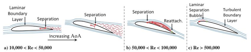
Abstract

Mars : The red planet has been on top in the priority list of interplanetary exploration of the solar
system. The Mars exploration landers and rovers have laid the foundation of our understanding
of the planet atmosphere and terrain. Although the rovers have been a great help, they also have
limitations in terms of their speed and exploration capabilities from the ground. Throughout the
whole mission period the rover is limited to travel for couple of Kilometers, and the lack of terrain
data in real time also limits the path planning of the exploration rovers. It would be beneficial in
terms of extended range of operation to have a secondary system that can fly ahead of the rover and
provide it with pre-mapped terrain so that the rover can select the optimal site to perform scientific
experiments. The INGENUITY Mars helicopter is designed to test the technical demonstration of
aerial flight in the thin atmosphere of Mars. This project will use some of the research and devel-
opments done for the ingenuity helicopter and aims to simplify the rotor craft’s design by adding
more rotors and getting rid of the variable pitch control used in ingenuity helicopter. In this thesis
we have proposed a multi rotor UAV that is developed for powered flight in the Mars atmosphere.
This thesis will give insights about the constraints and solutions to allow an autonomous UAV to
fly in the thin atmosphere of Mars. The thesis will focus on the selection of the optimal airfoil for
low Reynolds number flow on Mars, its aerodynamics which will be followed by flow simulations
in CFD software to extract thrust parameters for the UAV. The later half of the thesis project will
be primarily focused on designing a low level controller for the UAV to execute some basic com-
mands like hold position, do roll,pitch and yaw movements and following a specific path. From
the control prospective the scope of this master thesis is to make a mathematical model of the Mars
UAV and design a PID controller for the vehicle. The project will conclude the simulations and
control response from the PID controller and as a future work an LQR and MPC can be developed
for the Mars UAV.

                                                                                            ii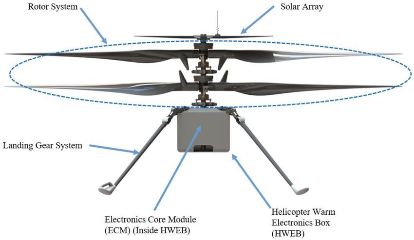
Table of Contents

1   Introduction                                                                                      1
    1.1   Motivation . . . . . . . . . . . . . . . . . . . . . . . . . . . . . . . . . . . . . . .    2
    1.2   UAV Flight in Mars Atmosphere . . . . . . . . . . . . . . . . . . . . . . . . . . .         3
    1.3   Thesis Outline . . . . . . . . . . . . . . . . . . . . . . . . . . . . . . . . . . . . .    4
          1.3.1    Chapter 2 . . . . . . . . . . . . . . . . . . . . . . . . . . . . . . . . . . .    4
          1.3.2    Chapter 3 . . . . . . . . . . . . . . . . . . . . . . . . . . . . . . . . . . .    4
          1.3.3    Chapter 4 . . . . . . . . . . . . . . . . . . . . . . . . . . . . . . . . . . .    4
          1.3.4    Chapter 5 . . . . . . . . . . . . . . . . . . . . . . . . . . . . . . . . . . .    4
          1.3.5    Chapter 6 . . . . . . . . . . . . . . . . . . . . . . . . . . . . . . . . . . .    5
          1.3.6    Chapter 7 . . . . . . . . . . . . . . . . . . . . . . . . . . . . . . . . . . .    5
          1.3.7    Chapter 8 . . . . . . . . . . . . . . . . . . . . . . . . . . . . . . . . . . .    5
          1.3.8    Chapter 9 . . . . . . . . . . . . . . . . . . . . . . . . . . . . . . . . . . .    5

2   Literature review and Background                                                                  6
    2.1   Computational Fluid Dynamics . . . . . . . . . . . . . . . . . . . . . . . . . . . .        6
          2.1.1    Reynolds Averaged Navier-Stokes equations . . . . . . . . . . . . . . . .          7
    2.2   Momentum theory of Rotors . . . . . . . . . . . . . . . . . . . . . . . . . . . . .         8
          2.2.1    Blade Element Momentum theory . . . . . . . . . . . . . . . . . . . . . . 12

3   Rotor blade optimization for Mars                                                                15
    3.1   Low Reynolds Number Aerodynamics . . . . . . . . . . . . . . . . . . . . . . . . 16
          3.1.1    Performance of Flat and Cambered Plate Airfoils . . . . . . . . . . . . . . 18
          3.1.2    Laminar and Turbulent Reattachments . . . . . . . . . . . . . . . . . . . . 19
          3.1.3    Ingenuity Helicopter . . . . . . . . . . . . . . . . . . . . . . . . . . . . . 21
          3.1.4    Performance Evaluation of Ingenuity Blade Profile . . . . . . . . . . . . . 22

4   Two Dimensional Flow Analysis                                                                    25
    4.1   Experimental Setup . . . . . . . . . . . . . . . . . . . . . . . . . . . . . . . . . . 25
          4.1.1    Turbulence and Laminar Separation Bubble Expectations . . . . . . . . . . 26
          4.1.2    Definition of 2D Geometry . . . . . . . . . . . . . . . . . . . . . . . . . . 27
    4.2   Result Validation of 2D Analysis . . . . . . . . . . . . . . . . . . . . . . . . . . . 28

                                                                                            iii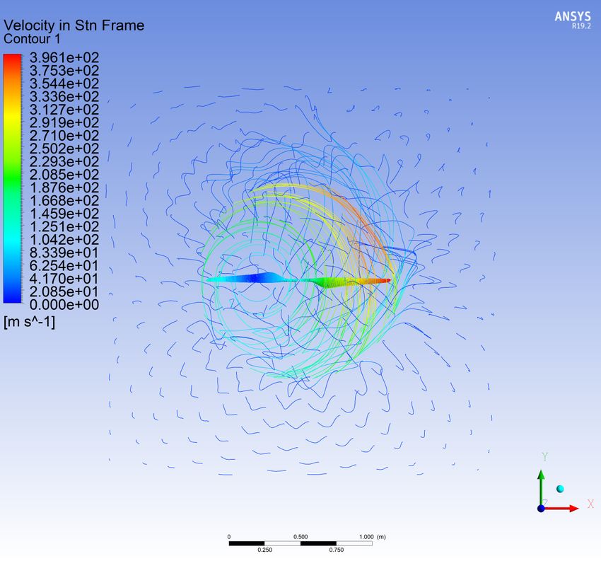
5   Fluent Simulation 3D                                                                          34
    5.1   Co-Axial Rotor System . . . . . . . . . . . . . . . . . . . . . . . . . . . . . . . . 34
    5.2   Simulation Setup In ANSYS Fluent . . . . . . . . . . . . . . . . . . . . . . . . . 35
    5.3   Simulation Results and Validation . . . . . . . . . . . . . . . . . . . . . . . . . . 36

6   CAD design of Mars UAV                                                                        43

7   Vehicle Dynamics                                                                              47
    7.1   Conventional Quadrotor . . . . . . . . . . . . . . . . . . . . . . . . . . . . . . . . 47
    7.2   Quadrotor Dynamics . . . . . . . . . . . . . . . . . . . . . . . . . . . . . . . . . 47
          7.2.1   Euler angles . . . . . . . . . . . . . . . . . . . . . . . . . . . . . . . . . . 50
          7.2.2   Mathematical Model of Quadrotor . . . . . . . . . . . . . . . . . . . . . . 51
    7.3   Mars UAV Model Dynamics . . . . . . . . . . . . . . . . . . . . . . . . . . . . . 53
          7.3.1   Equations of Motion . . . . . . . . . . . . . . . . . . . . . . . . . . . . . 55
          7.3.2   State Space Representation . . . . . . . . . . . . . . . . . . . . . . . . . . 56

8   Mars UAV System Control                                                                       60
    8.1   Open Loop Simulation . . . . . . . . . . . . . . . . . . . . . . . . . . . . . . . . 60
          8.1.1   Motor Mixer Subsystem . . . . . . . . . . . . . . . . . . . . . . . . . . . 62
          8.1.2   Rotation Subsystem . . . . . . . . . . . . . . . . . . . . . . . . . . . . . 63
          8.1.3   Translation Subsystem . . . . . . . . . . . . . . . . . . . . . . . . . . . . 64
    8.2   Closed Loop Simulations . . . . . . . . . . . . . . . . . . . . . . . . . . . . . . . 65
          8.2.1   Altitude Controller . . . . . . . . . . . . . . . . . . . . . . . . . . . . . . 65
          8.2.2   Heading and Attitude Controller . . . . . . . . . . . . . . . . . . . . . . . 65
          8.2.3   Position Controller . . . . . . . . . . . . . . . . . . . . . . . . . . . . . . 66
    8.3   PID Control . . . . . . . . . . . . . . . . . . . . . . . . . . . . . . . . . . . . . . 68
          8.3.1   Altitude PID Control . . . . . . . . . . . . . . . . . . . . . . . . . . . . . 69
          8.3.2   Roll PID Control . . . . . . . . . . . . . . . . . . . . . . . . . . . . . . . 69
          8.3.3   Pitch PID Control . . . . . . . . . . . . . . . . . . . . . . . . . . . . . . . 70
          8.3.4   Yaw PID Control . . . . . . . . . . . . . . . . . . . . . . . . . . . . . . . 71
          8.3.5   Position PID Control . . . . . . . . . . . . . . . . . . . . . . . . . . . . . 72
    8.4   Simulation Results for PID Control . . . . . . . . . . . . . . . . . . . . . . . . . . 73
          8.4.1   Position response . . . . . . . . . . . . . . . . . . . . . . . . . . . . . . . 74
          8.4.2   Trajectory Follow response . . . . . . . . . . . . . . . . . . . . . . . . . . 75

9   Conclusion                                                                                    79

                                                                   TABLE OF CONTENTS      iv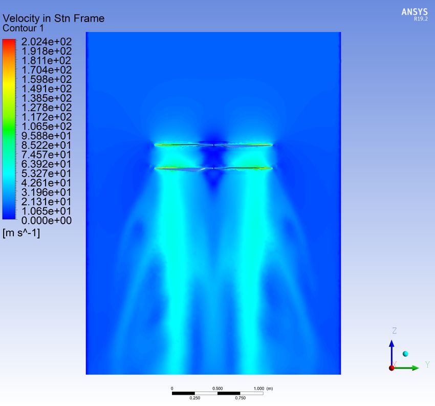
List of Figures

 2.1   Control volume for streamtube representation . . . . . . . . . . . . . . . . . . . .       9
 2.2   Aerodynamic forces on blade profile . . . . . . . . . . . . . . . . . . . . . . . . . 12

 3.1   subsonic and transonic airfoils . . . . . . . . . . . . . . . . . . . . . . . . . . . . 15
 3.2   Flow separation affected by Reynolds number and angle of attack . . . . . . . . . 16
 3.3   CL vs Reynolds number . . . . . . . . . . . . . . . . . . . . . . . . . . . . . . . 18
 3.4   CD vs Reynolds number . . . . . . . . . . . . . . . . . . . . . . . . . . . . . . . 18
 3.5   Separation bubble . . . . . . . . . . . . . . . . . . . . . . . . . . . . . . . . . . . 20
 3.6   Ingenuity Helicopter . . . . . . . . . . . . . . . . . . . . . . . . . . . . . . . . . 22
 3.7   Performance of Ingenuity helicopter test model for different atmospheric conditions 23

 4.1   Geometry of flat plate defined in grid . . . . . . . . . . . . . . . . . . . . . . . . . 27
 4.2   Geometry of cambered plate defined in grid . . . . . . . . . . . . . . . . . . . . . 27
 4.3   Cl versus Cd for a flat plate . . . . . . . . . . . . . . . . . . . . . . . . . . . . . . 28
 4.4   Angle of attack versus Cl and Cd for flat plate . . . . . . . . . . . . . . . . . . . . 29
 4.5   Lift/Drag coefficients versus Angle of attack for flat plate . . . . . . . . . . . . . . 29
 4.6   Angle of attack versus Cl and Cd for cambered plate . . . . . . . . . . . . . . . . 30
 4.7   Lift/Drag coefficients versus Angle of attack for cambered plate . . . . . . . . . . 30
 4.8   (a) Velocity profile over cambered plate airfoil (b) Velocity profile over ACA airfoil
       (c) Velocity profile over a DEP airfoil (d) Velocity profile over PAT airfoil . . . . . 31
 4.9   (a) Laminar boundary layer at angle of attack α = 0° (b) shear layer separation
       Angle of attack α = 2° . . . . . . . . . . . . . . . . . . . . . . . . . . . . . . . . 31
 4.10 (a) Shear layer behaviour at angle of attack α = −2° (b) shear layer behaviour at
       Angle of attack α = −3° . . . . . . . . . . . . . . . . . . . . . . . . . . . . . . . 32
 4.11 Extreme mach number in subsonic range showing shock wave formation . . . . . . 33

 5.1   (a) Thrust plot for a single rotor (b) Velocity contour with flow lines for a single rotor 36
 5.2   Velocity in stationary frame contour for co axial rotors . . . . . . . . . . . . . . . 38
 5.3   Maximum velocity value in stationary frame for 3000 rpm . . . . . . . . . . . . . 39
 5.4   Force report from Fluent . . . . . . . . . . . . . . . . . . . . . . . . . . . . . . . 39
 5.5   Pressure contours for co axial rotors . . . . . . . . . . . . . . . . . . . . . . . . . 40

                                                                                          v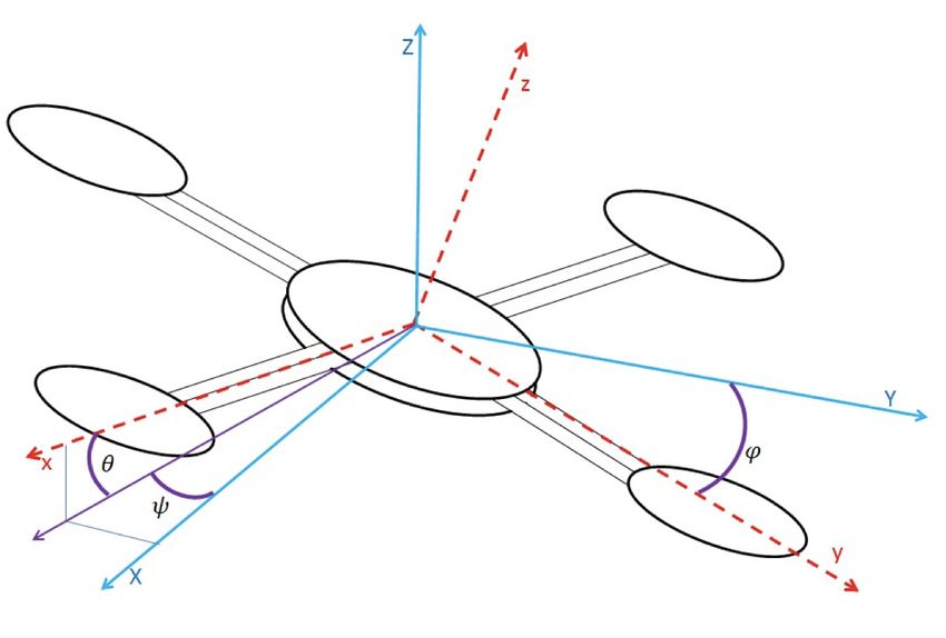
5.6   Global velocity contour with streamlines . . . . . . . . . . . . . . . . . . . . . . . 41
5.7   (a) Velocity contour lines on rotor surfaces (b) Pressure contour lines on rotor
      surfaces . . . . . . . . . . . . . . . . . . . . . . . . . . . . . . . . . . . . . . . . 42

6.1   Isometric view of the Mars UAV model . . . . . . . . . . . . . . . . . . . . . . . 43
6.2   Rotor blade of Mars UAV . . . . . . . . . . . . . . . . . . . . . . . . . . . . . . . 44
6.3   Side view : Rotor blade of Mars UAV . . . . . . . . . . . . . . . . . . . . . . . . 44
6.4   Subsystems Mars UAV model . . . . . . . . . . . . . . . . . . . . . . . . . . . . 45

7.1   World and Body frame of reference for a quadrotor . . . . . . . . . . . . . . . . . 48
7.2   Differential thrusts for roll, pitch and yaw moments . . . . . . . . . . . . . . . . . 49
7.3   Euler angles representation . . . . . . . . . . . . . . . . . . . . . . . . . . . . . . 51
7.4   Mars UAV rotors representation . . . . . . . . . . . . . . . . . . . . . . . . . . . 53

8.1   Block diagram of open loop simulation . . . . . . . . . . . . . . . . . . . . . . . . 61
8.2   Motor mixer subsystem for open loop simulation . . . . . . . . . . . . . . . . . . 62
8.3   Rotation subsystem for open loop simulation . . . . . . . . . . . . . . . . . . . . 63
8.4   Translation subsystem for open loop simulation . . . . . . . . . . . . . . . . . . . 64
8.5   Block diagram of the Altitude controller . . . . . . . . . . . . . . . . . . . . . . . 65
8.6   Block diagram of the Attitude and Heading controller . . . . . . . . . . . . . . . . 66
8.7   Block diagram of the Position controller . . . . . . . . . . . . . . . . . . . . . . . 67
8.8   Block diagram of the PID controller . . . . . . . . . . . . . . . . . . . . . . . . . 68
8.9   Block diagram of the altitude PID controller . . . . . . . . . . . . . . . . . . . . . 69
8.10 Block diagram of the Roll PID controller . . . . . . . . . . . . . . . . . . . . . . . 70
8.11 Block diagram of the Pitch PID controller . . . . . . . . . . . . . . . . . . . . . . 71
8.12 Block diagram of the Yaw PID controller . . . . . . . . . . . . . . . . . . . . . . 72
8.13 Altitude response PID control . . . . . . . . . . . . . . . . . . . . . . . . . . . . 73
8.14 Control responses from PID controller . . . . . . . . . . . . . . . . . . . . . . . . 74
8.15 Square trajectory follow response . . . . . . . . . . . . . . . . . . . . . . . . . . . 75
8.16 Control responses for square trajectory follow with PID control . . . . . . . . . . . 76
8.17 Helix trajectory follow response . . . . . . . . . . . . . . . . . . . . . . . . . . . 77
8.18 Control responses for helix trajectory follow with PID control . . . . . . . . . . . 78
8.19 Simulink Model of Mars UAV . . . . . . . . . . . . . . . . . . . . . . . . . . . . 78

                                                                   LIST OF FIGURES    vi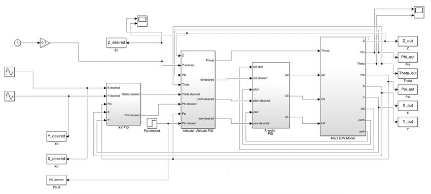
List of Tables

 3.1   Mean Atmospheric Properties . . . . . . . . . . . . . . . . . . . . . . . . . . . . 15
 3.2   Mars conditions for test articles . . . . . . . . . . . . . . . . . . . . . . . . . . . . 24

 4.1   Angle of attack (AOA) and Mach numbers for different radial stations . . . . . . . 26

 7.1   States representation . . . . . . . . . . . . . . . . . . . . . . . . . . . . . . . . . 57

 8.1   PID position inputs and gains . . . . . . . . . . . . . . . . . . . . . . . . . . . . . 74

                                                                                        vii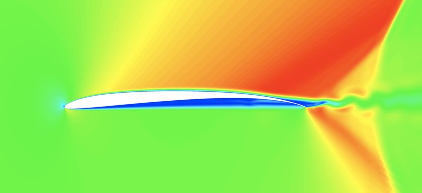
Acronyms

UAV : Unmanned Aerial Vehicle
MRO : Mars Reconnaissance Orbiter
CFD : Computational Fluid Dynamics
LQR : Linear Quadratic Regulator
MPC : Model Predictive Control
PID : Proportional Integral Derivative
INGENUITY : Mars Helicopter
ACA : Arbitrary Continuous Airfoil
DEP : Double Edged Plate

                                         viii
Nomenclature
c = Airfoil chord
CL = Lift coefficient
Cd = Drag coefficient
g = Gravitational acceleration
M = Mac number
R = Gas constant
γ = Specific heat ratio
Re = Reynolds number
α = Angle of attack
t = Airfoil thickness
Ω = Rotor speed
m = Mass
φ = Roll angle
θ = Pitch angle
ψ = Yaw angle
k p = Proportional gain
ki = Integral gain
kd = Derivative gain
V = Velocity in inertial frame
VB = Velocity in Body frame
ω = Angular velocity
p = Roll rate
q = Pitch rate
r = Yaw rate
ixChapter 1
Introduction
The idea of exploration fulfils human curiosity in order to find answers to the science mysteries
present in the Universe. The question that has been pursued over many years now is: how did life
evolve in our solar system, and other than Earth where else life could have existed in the early
days of our solar system formation? These questions lead us to identifying the habitable zone of
our solar system and the planets that fall under this habitable zone. Earth and Mars are prime
candidates for satisfying the criteria defined to be in the habitable zone of the solar system. For
many years now we have been sending unmanned robotic probes, orbiters, landers and rovers to
the red planet Mars in order to understand its composition, atmosphere, geology etc. There have
been over 45 missions that were targeted to Mars by collective effort from different space agencies
from around the world. The unmanned robotic missions are great at exploring the red planet while
also surviving the harsh atmosphere environment and radiation dose. The robotic exploration has
paved the way for humanity to research technology that supports human settlement on Mars. The
rovers Spirit and Opportunity have led a foundation for developing technology to send robust and
autonomous systems to conduct experiments on Mars. The orbiters have mapped the surface of
the planet with great detail that helps space agencies in selecting landing sites of future missions
in order to define mission objectives, and also to have knowledge about the environment in which
the lander or rover will be performing experiments. The orbiters like Mars Reconnaissance Or-
biter (MRO) and Mars Express have mapped the interesting regions of the planet like Volcanoes,
Canyons and polar ice caps. Even after using the best quality Hires Images from MRO, the sur-
face has only been mapped with resolution of about 20 m per pixel. For this purpose the rovers
have been designed and sent to Mars in order to partially fill the data gaps from the orbiters. The
rovers have been successful in doing onsite research about mineral composition of rocks and soil,
1atmospheric studies along with sending beautiful panoramic mosaics of the red planet. The rovers
are still limited by their ability to move quickly from one site to another site of interest in order to
conduct science experiments.
1.1 Motivation
The limitation posed by ground based exploration vehicles are a constraint to going further on the
red planet. In order to overcome this limitation, the idea of aerial exploration has been considered
for many years and many methods have been proposed to go a step further by changing the mode
of exploration. Aerial exploration is great at moving from point A to point B without consid-
erations about the terrain and ground obstacles. Aerial exploration also allows for movement at
higher speeds from one site to another site of interest. There have been many ideas and theories
that propose modes of transport that consider flying or hovering vehicles. Among many projects
considered for developing multi rotor systems to fly on Mars, the project that has been an inspir-
ation to this thesis is the Ingenuity Mars helicopter project. [1] The Mars helicopter is a small,
lightweight helicopter design that has been designed and tested by JPL in NASA in a simulated
environment that represent atmosphere, density, pressure and gravity in Mars-like conditions. This
master thesis is based on two aspects of designing a multi rotor Unmanned Aerial Vehicle for Mars
exploration. The first aspect of the project will focus on studying the thin atmosphere aerodynam-
ics on Mars and proposing a blade profile for a Mars UAV and also designing a CAD model of the
UAV for CFD simulations. The other aspect of the thesis will focus on modelling the equations
of motion for an octa-rotor coaxial UAV, designing a PID controller and simulating the model in
SIMULINK to perform some basic autonomous task like hovering, following a trajectory etc. The
technological demonstration about making the first powered flight in the Mars atmosphere from
the Ingenuity helicopter will build a foundation for developing autonomous control for rotor crafts
for space purposes. There have been a significant amount of research done by JPL and Caltech
in order to develop thin airfoil aerodynamics analysis that focuses on low Reynolds number flow.
A significant part of these studies have been conducted for the Ingenuity helicopter project. This
Introduction 2thesis project will take inspiration from the Ingenuity helicopter and develop a multi rotor system
that will be able to make an autonomous flight in the Mars atmosphere.
1.2 UAV Flight in Mars Atmosphere
Mars has a very challenging atmosphere in terms of temperature fluctuations, dust storms, surface
composition that limits the locations that Mars exploration rovers can reach. The concept of UAVs
to fly on Mars is proposed to prove that with considerable optimization in rotor blade design,
enough lift can be generated to fly a lightweight UAV in the thin atmosphere. The concept also
focuses on making the flight and operation autonomous, mapping the surrounding terrain, and
path planning to assist the ground based rover to reach beyond its current capabilities. The Mars
UAV will operate in the conditions where the tip Mach numbers are high and Reynolds number
is low. In a generic rotor design, it is important to maintain subsonic speed at the tip of the rotor
in order to avoid undesired shock wave formation. The generated shock waves highly affect the
lift generation capabilities of the rover if not considered beforehand. Because the atmospheric
density is very low on Mars, there is a benefit in spinning the rotor at higher RPM and still keep
the tip speeds subsonic. The hovering of the vehicle will be controlled in a similar manner to
any quadrotor that flies in Earth conditions. The roll, pitch and yaw movement commands will
be handled by the proposed PID controller that will be designed specially to control the co-axial
rotors. The reduced value of gravity will help the vehicle remain stable when flying and will
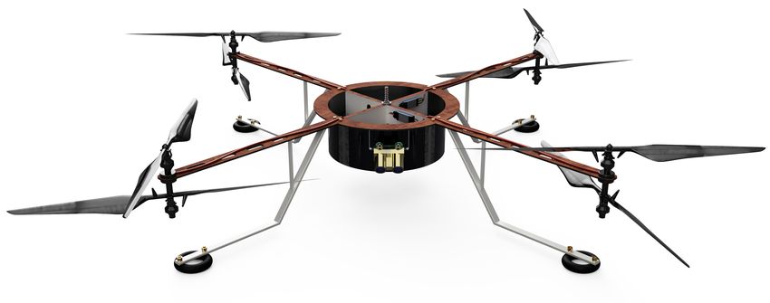
minimise small instabilities caused by the frequencies of unstable phugoids [2]. The proposed size
of the rotor blade is 1.12 meters and two rotors spin in opposite directions when mounted in a
co-axial manner. This approximation estimate the overall UAV mass to be around 6 Kilograms.
Parts of the on board payload and system requirements will be discussed in the CAD modelling
part of this project. Currently the Mars rovers that are operating on Mars are powered by RTG
(Radioisotope Thermo electric Generator), But because the RTGs have very low efficiency, they
are not suitable for UAV because of the heavy subsystem required to manage the heat produced by
RTG. The Mars UAv is designed to get its power from solar energy. The larger arms of the Mars
UAV are suitable to mount roll out solar arrays on them. These solar arrays can be extended for
charging and can be retracted during flying. Flight data from the Ingenuity helicopter project will
Introduction 3clarify whether or not a powered fight is possible in Mars atmosphere, and will help this idea to be
pursued in terms of increasing the payload mass and decreasing system mass [1].
1.3 Thesis Outline
1.3.1 Chapter 2
This chapter of the master thesis will give insights to the basics of computational fluid dynamics
and Navier-Stokes equations. The goal of the literature review on reynolds averaged Navier-Stokes
equations is to adapt the understanding of RANS for low reynolds number flow simulations. This
chapter also talks about the generic and blade element momentum theory of rotors.
1.3.2 Chapter 3
In this chapter the low reynolds number aerodynamics in thin atmosphere has been studied. The
flow performances of flat and cambered plates has been studied in order to optimize for delayed
transition from laminar to turbulent flow. This section of the thesis also talks about the Mars
Helicopter project that has been developed by JPL to make a helicopter model for a tech demo on
UAV flight in Mars atmosphere.
1.3.3 Chapter 4
This chapter of the thesis project shows the simulation results for two dimensional flow around flat
plate, cambered plate and Ingenuity helicopter rotor blade airfoil. In this chapter the studies from
different authors is compared for optimizing a 2D airfoil for low reynolds number flow. The effects
of high mach number around the rotor tips is also described in this chapter.
1.3.4 Chapter 5
In this chapter the simulation results from Ansys fluent are presented. The Mars condition simula-
tion for flow around the single and co-axial rotor system is considered to see the effects of different
RPM values and optimize for best rotor speed to produce necessary thrust.
Introduction 41.3.5 Chapter 6
In this chapter a CAD model of the Mars UAV is presented. The different subsystems of the model,
the vehicle structure and power system is described in this section.
1.3.6 Chapter 7
In this section of the master thesis, the dynamics of a UAV model is described. Conventional
quadrotor is taken as reference in order to describe the mathematical model of the Mars UAV.
1.3.7 Chapter 8
This section of the thesis introduces control strategies for the Mars UAV. Open loop and closed
loop simulations were performed and the model was extended to implement a PID controller to
record the response of the Mars UAV model for a trajectory following task.
1.3.8 Chapter 9
The final chapter of the master thesis considers concluding remarks from the work done on the
design and control of Mars UAV. Learning outcomes and future control implementations are also
suggested for the Mars UAV.
Introduction 5Chapter 2
Literature review and Background
In order to explain the work done in this thesis on the flow simulations part, it is necessary to
introduce the basics of fluid dynamics, CFD, Quadrotor equations of motions etc. The concept
of a Mars UAV is proposed to operate in incompressible flow conditions and for that the used
Navier-Stokes equations are from the incompressible set of equations. For numerical simulations
and model building, the Fluent from ANSYS software is used. The 2D analysis of the different
airfoils are performed using the Xfoil tool.
2.1 Computational Fluid Dynamics
Computational Fluid Dynamics is based on the Navier-Stokes equations that are used to model
numerical solutions to describe flow behaviours. These are also key equations to understand flow
interactions around solid surfaces. The numerical model derived from Navier-Stokes equations
is beneficial in terms of doing a simulation for the Mars condition before fabricating the model
for lab experiment. Because of evolving technology and modern computers, the time required to
simulate the flow has been greatly reduced and complex experiments can be modeled inside a CFD
environment before the actual experiments.
Using the three fundamental laws of physics, which are conservation of mass, conservation of
energy and newton’s second law of motion; the Navier-stokes equations create set of partial dif-
ferentiation equations. In order to solve for primary flow variables that are pressure and velocity,
the conservation of mass and conservation of momentum are sufficient. The energy conservation
is necessary when the compressible flows are discussed. Since this thesis is only focusing on
the incompressible flows, we will not discuss the energy equations. The law of conservation of
6mass states that mass can not be created not destroyed. So for the incompressible flow, the net
flow entering the boundary volume is equal to the net flow leaving the volume. The boundary
volume is a box shaped enclosure defined in the CFD set up. The dimensions of the volume are
3400 × 1500 × 1500 mm3
∂ ρ ∂ (ρui )
+ =0 (2.1)
∂t ∂ xi
The equation (2.1) is called the continuity equation in aerodynamics. The flow considered is the
incompressible flow thus the density does not change over time.
∂ρ
=0 (2.2)
∂t
Therefore,
∂ (ρui )
=0 (2.3)
∂ xi
Newton’s second law of motion says that the total force is equal to the change in momentum over
time. The conservation of momentum for the defined volume is defined by the equation (2.4) in
Cartesian coordinates frame.
∂ (ρui ) ∂ [ρui u j ] ∂ p ∂ τi j
+ =− + + ρ fi (2.4)
∂t ∂xj ∂ xi ∂ x j
Where, τ is stress, ρ is density, p is pressure u, v and w are the velocity component in x,y and x
directions respectively. velocity and f is the force.
2.1.1 Reynolds Averaged Navier-Stokes equations
In fluid mechanics an instantaneous solution is not preferred in most of the areas and instead an
average solution is computed from the set of equations described earlier. The purpose of RANS
is also to separate the turbulent and laminar components in the flow equations. By inputting the
Literature review and Background 7expected values of RHS and LHS, on all four equations and simplifying according to the rules of
expectation, the Reynolds Averaged Navier-Stokes equations are derived as,
∂ ui
=0 (2.5)
∂ xi
∂ ui ∂ ui 1 ∂p ∂ 2 ui
+uj = fi − +ν (2.6)
∂t ∂xj ρ ∂ xi ∂ x j∂ x j
Averaging on the right and left hand sides of the equation (2.6) we get,
0 0
∂ ūi ∂ ūi 1 ∂ p̄ ∂ 2 ūi ∂ ui u j
+ u¯j = f̄i − +ν − (2.7)
∂t ∂xj ρ ∂ xi ∂ x j∂ x j ∂xj
In the equation (2.7), ui is the averaged value of velocities in the Cartesian x, y and z directions
and fi denotes the total forces acting on the bounding volume. The new set of equations referred
to as Reynolds Averages Navier-Stokes equations introduces 6 new unknown variables due to
the symmetric Reynolds stress tensor [2]. Including the new set of equations, there are total 10
unknown variables are present. There are only four equations to solve for 10 unknown variables
thus, In order to derive the amount of equations needed, the evolution equations of the stress tensor
needs to be derived. Since this goes out of the focus of this thesis, the derivation of the remaining
equations will not be discussed in this thesis.
2.2 Momentum theory of Rotors
The interest within the robotics community has peaked recently in order to understand the aero-
dynamics of quadrotors to improve the rotor efficiency by including the lift and drag parameters
into the mathematical models. The studies in this field have only been focused on the theory of
momentum for helicopters and indeed more detailed studies of rotor blade aerodynamics is neces-
sary in order to include the aerodynamic parameters into the vehicle from a control prospective.
[3] The momentum theory for rotary wing was developed in the early stage for aircraft propellers.
It is considered as one of the most widely used theories in the field of propeller analysis for sub-
Literature review and Background 8sonic flights. The simple approach of the theory has made it the base foundation for modelling the
aerodynamic forces on rotors. This theory considers the rotor as an actuating disk with with the
accelerating fluid medium forming a stream tube in the axial direction. The visual representation
of the stream tube can be seen in Figure 2.1. The working fluid (normally air) is sucked and ac-
celerated by the rotors in the downward direction which generates a virtual induced flow of fluid
which has velocity vi = (vix , viy , viz )T [3].
Figure 2.1: Control volume for streamtube representation
The disk loading is defined as the ratio between the Thrust and disk Area.
T
DL = (2.8)
A
According to the assumptions made in the momentum theory, it is clear that the the higher the disk
loading values the more likely the assumptions will hold [3]. For quadrotors, the observed value
of disk loading is higher as compared to the helicopters and thus the momentum theory fits better
Literature review and Background 9for quadrotors than it does for the helicopter vehicles. The fluid flow velocities have generic form
in the Cartesian system, thus it is recommended to consider a single direction in order to optimize
the flow equations. The discussion is based on the flow conditions in the axial or Z direction.
From the Figure 2.1(Courtesy of Bangura [3] the velocity in the axial Z direction can be defined as
V = (0, 0,Vz )T .
The fluid flow through the rotor disc is continuous and is given by a constant speed at which the
vehicle hovers. This speed is defined as the induced velocity in the Z direction or is denoted by
vi . When the rotor disc is spinning there is a pressure gradient observed on the inlet and outlet
sides and this pressure gradient is denoted by ∆P. The bounding volume that is defined to contain
the rotor disk has a radius of R0 where the radius of the rotor disk is R. The bounding volume is
defined with the intention to compute the amount of fluid entering from the inlet and leaving from
the outlet. The upstream plane has radius R0 and the downstream plane has the radius of r < R.
It is obvious that is has a lesser radius on the outlet side due to the pressure gradient generated
and the flow lines shrink as they pass through the rotor. The assumption made here implies the the
flow stream lines are parallel with the axial Z axis or the rotor spin axis. The thrust force can be
computed from the equation of momentum theory by considering the difference in mass flow per
volume. This gives the following equation (2.9),
T = ṁ(Vz∞ −Vz ) − ṁ(−Vz ), = ṁVz∞ (2.9)
Where ṁ is the mass flow rate and the mass flow rate is given as
ṁ = ρA|V a | (2.10)
Where,
0
a
V = (2.11)
0
viz −Vz
Literature review and Background 10Because the mid section radius of the stream tube and the radius of the rotor are same, the cross
section area is given by A = πR2 . The power can be calculated from the force and velocity. The
force here is considered as thrust force thus,
PT = T (viz −Vz ) (2.12)
This power can also be considered as equivalent to the change in the kinetic energy at the inlet and
outlet. Therefore the equation (2.12) can also be written as,
1 1
PT = ṁ(Vz∞ −Vz )2 − ṁ(Vz )2 ,
2 2
1 1
PT = ṁ(Vz2 − 2VzVz∞ + (Vz∞ )2 − (Vz )2 . (2.13)
2 2
From the equations (2.9) and the equations (2.12) the equation (2.13) can be modified and written
as,
1
ṁVz∞V a = ṁ((Vz∞ )2 − 2VzVz∞
2
Therefore,
1
viz = Vz∞
2
And the equations for Thrust power and Thrust force can be derived as,
T = 2ρAviz (viz −Vz ), (2.14)
PT = T (viz −Vz ) (2.15)
The equations (2.14) and (2.15) are considered as the Thrust and Thrust power in the axial or Z
direction of the fluid flow. The direction of rotor spinning is also considered to be the same as the
Literature review and Background 11Z-axis. These equations [3] give the values in steady state and in one direction of fluid flow motion.
If needed, the equations for generic motion of the rotor disk can also be derived by referring to the
equations (2.14) and (2.15). The generic motion of rotor is not discussed here because it is out of
scope of the research for this thesis.
2.2.1 Blade Element Momentum theory
In the generalised momentum theory, there have been number of assumptions made which make
it less reliable to extract flow parameters. For this purpose Blade Element theory was proposed.
The blade element theory uses the geometrical profile of the cross section of the rotor in order to
compute aerodynamic forces acting on the rotor. This results in a higher number of equations to
solve for the Forces and Moments. The rotor twist distribution is also taken into consideration in
the blade momentum theory.
Figure 2.2: Aerodynamic forces on blade profile
In the blade element theory also a stream tube is considered to be the control volume inside which
a rotor is placed. In the plane of the rotor, the boundaries of the stream tube splits the rotor into
number of elements with the width given as dr collectively representing the rotor blade section. At
every blade element the differential thrust can be defined as dT and can be defined for the particular
cross-section of that element. The torque is given as dQ. From Figure 2.2(courtesy of Rwigema
[4]) it can be seen that in order to compute the Thrust and Torque, equations need to be written
in term of the angle of attack which is given by the angle φ . From here on, the angle of attack
is defined for each element of the rotor blade which is being considered to calculate total thrust
Literature review and Background 12and torque. From the Figure 2.2 the incremental thrust and torque is given as equations (2.16) and
(2.17).
1
dT = BρU 2 (CL cos φ −CD sin φ )cdr (2.16)
2
1
dQ = BρU 2 (CL sin φ +CD cos φ )crdr (2.17)
2
Aerodynamic performance of a rotor can be computed from the combination of the equations
derived in the Momentum theory and the Blade Element theory. For this the blade profile or airfoil
shape, twist distribution are assumed to be known. By further modifying the equations (2.16) and
(2.17), the thrust and torque can be defined in terms of the known variables from the Figure 2.2.
V∞2 (1 + a)2
dT = σ 0 πρ (CL cos φ −CD sin φ )rdr
sin2 φ
V∞2 (1 + a)2
dQ = σ 0 πρ 2
(CL sin φ +CD cos φ )r2 dr
sin φ
In this thesis, aerodynamic analysis plays a crucial role in quadrotor performance. The BEMT
(Blade Element Momentum Theory) gives accurate values of aerodynamic coefficients in order to
model them into the numerical analysis to get the rotor performance. On Mars the flow is assumed
to be incompressible and the analysis is done for the low Reynolds number flow, additionally
the aerodynamic coefficients are affected by the viscosity effects. This is also part of the reason
for considering the Viscous model in Fluent while simulating the rotor blade in ANSYS. In this
thesis, XFOIL tool is used to consider the viscosity effects. In XFOIL it is possible to input the
Reynolds number and tip mach number as input in order to get the viscosity information of the
flow. Reynolds number define the property of the flow in terms of streamline behaviour of the flow
and the Mach number gives the ratio of velocity to the speed of sound in the considered medium
of analysis.
Literature review and Background 13ρV∞ c
Re = (2.18)
µ
V∞
M=√ (2.19)
γRT
Literature review and Background 14Chapter 3
Rotor blade optimization for Mars
This chapter of the thesis will briefly talk about the importance of blade profile optimization for
the low Reynolds number and high mach number flow in Martian atmospheric conditions. Mars
surface pressure is very low as compared to Earth, thus the blade profiles in the directory of NACA
series is not as efficient in providing the required lift as they are designed to operate in Earth
conditions.
(a) Subsonic NACA 0012 airfoil (b) High Mach number CLF 5605 Airfoil
Figure 3.1: subsonic and transonic airfoils
The comparison between the subsonic and transonic airfoils are shown in Figure 3.1. The NACA
series airfoils are widely used in rotor designs for multi rotor crafts. The twist distribution also
plays an important role in providing correct geometry for optimized aerodynamic coefficients. The
atmospheric conditions of considered Mars and Earth atmosphere are mentioned in the table 3.1.
Parameter MARS EARTH
Density (Kg/m3 ) 0.00155 1.23
Pressure (Pa) 636 101325
Temperature (K) 214 288
Speed of Sound (m/s) 230 340
Gamma, γ 1.3 1.4
Table 3.1: Mean Atmospheric Properties
15The lower value of lift generated by a rotor in Mars atmosphere is partially compensated by the
low gravity of the planet. This means that there is a slight advantage to the rotor craft flying in
Mars atmosphere because the gravitational acceleration is low compared to Earth. The drawback is
the temperature and atmospheric composition of Mars. The average surface temperature on Mars
is about 214 K and the atmosphere is mostly (95%) composed of CO2. This results in lower speed
of sound based on equation 2.19. The challenge of lower speed of sound constrains the maximum
tip speed that the rotor can achieve because the lower the speed of sound, the sooner the flow
becomes supersonic. As soon as the flow crosses the subsonic limit, the undesired shock waves are
generated. These shock waves drastically increase the leading edge drag force and decreases the
overall aerodynamic lift-generating capabilities of the rotor. Prior research in airfoil optimization
and 2D flow analysis is needed in order to further advance the existing performance values of blade
profiles in low Reynolds number flow conditions.[5][6]
3.1 Low Reynolds Number Aerodynamics
The need for considering the low Reynolds number aerodynamics for the Mars UAV is discussed
in the previous sections. When dealing with the low Reynolds number flow, the boundary layer
is assumed to be fully laminar up to the point at which it separates from the rotor surface. The
subsequent turbulent flows are not observed until the point of separation this is mainly because
the separation point is delayed further towards the trailing edge when low reynolds number and
low angle of attack are considered. In Figure 3.2, the laminar flow separation points are seen for a
range of Reynolds number as well as with the change in angle of attack.
Figure 3.2: Flow separation affected by Reynolds number and angle of attack
At this stage it is important to understand the critical Reynolds number. The critical Reynolds
Rotor blade optimization for Mars 16number is defined as the Reynolds number at which the laminar flow is transitioning towards the
turbulent behaviour. The super critical Reynolds number is defined as the the range of Reynolds
number where the turbulent transition is always occurring before the laminar flow separation. Be-
cause the understanding of compressible flow at low Reynolds number is limited, the detailed study
is not usually performed because it is not coherent with the scientific goal of doing aerodynamic
analysis for Mars atmosphere conditions. This is mainly because the flow considered for the Mars
UAV is incompressible. The generic series of NACA airfoils are sensitive to change in Mach num-
ber where as the flat plate and cambered airfoils flow is not heavily mach number dependant.[5][6]
The region of transition between the sub critical and super critical Reynolds number flow is chal-
lenging because of the external disturbances, vibrations and the anomalies on the smoothness of
the surface.[7][8][9] The reason for flat plates and cambered airfoils are not highly dependent on
the Reynolds number is observed to be because of the sharp leading edge of the airfoils compared
to the conventional airfoils.[7] Even if the cambered plates are not dependent on the flow Reyn-
olds number, it is difficult to carry out analysis with conventional methods due to the leading edge
flow separation on these airfoils. In the modelling when the flow Reynolds number is significantly
decreased, the separation layer has the ability to reattach and this is because the sharp leading
edge not allowing the generated shear layer to transition from laminar to turbulent. In the previ-
ous research, this laminar streamline re-attachments is seen for the flat plate aerodynamics for the
Reynolds number range of approximately 10,000 [10][11].
The laminar to turbulent transitions are not only limited to the leading edge of the flat plates but are
also observed in the trailing edge of the airfoils. This behaviour is referred as vortex shedding and
is normally observed near sharp edges or surfaces with uneven geometry. The vortices are formed
due to the instabilities present in the flow and are also observed at the flow separation regime of the
airfoils. The pressure gradient also plays an important role here in the formation of the shedding
vortices. The laminar to turbulent transition is considered as minor anomaly as compared to the
significance of the shedding vortices formed in the low Reynolds number analysis[12].
Rotor blade optimization for Mars 173.1.1 Performance of Flat and Cambered Plate Airfoils
Flat plates that have a leading edge that is sharp have different performance than the conventional
airfoils in low Reynolds number. In-depth studies on this behaviour suggest that the transitioning
region from laminar to turbulent differs when flat plate and a conventional airfoil is considered.
The studies from Hoerner [13] shows that the lift coefficient for a cambered plate is lower than the
lift coefficient for the N60 airfoil. However the CL is observed to decrease by a very small amount
for the flat plate as compared to the N60 airfoil when the low Reynolds number is considered. The
plot in Figure 3.3 and Figure 3.3 (courtesy of Koning[14] and Hoerner[13]) shows the behaviour
of lift coefficient CL with varying Reynolds number of the flow.
Figure 3.3: CL vs Reynolds number
Figure 3.4: CD vs Reynolds number
Rotor blade optimization for Mars 18The thickness to chord ratio of an airfoil represents the thickness of the airfoil at different distances
from the leading edge. This ratio is a key parameter when examining the performance of airfoil
at transonic speeds. This behaviour is observed at constant angle of attack and the flat plates that
are considered for this analysis have the ratio of thickness to chord as 3%. The airfoil camber
for the flat plate is 5.8%. These values for the considered N60 airfoil are 12.4% and 4% respect-
ively.[14][13] From the Figure 3.3 and Figure 3.3 is is observed that the Lift coefficient and the
Drag coefficient is nearly independent of change of the Reynolds number in the range of 104 to
106 . The sharpness of the leading edge has an effect on the location of the separation point. The
stagnation point is defined as the point on the airfoil surface at which the free stream velocity be-
comes zero. One stagnation point occurs at the leading edge and the other occur at the trailing edge
of the airfoil. With the increase in the angle of attack, the stagnation point changes position and is
moved towards the lower surface. This creates turbulent behaviour in the flow and this allows for
a longer range of Reynolds number before the super critical Reynolds number is reached. When
the angle of attack is fixed and is not varying, then the flow does not show the transition occur-
ring at the super critical Reynolds number because the flow breaking point is shifted downwards.
The turbulent edge of the flow always occurs at the same point for all non zero angles of attacks
[7]. The turbulent transition flow characteristic is observed at x/c = 2.5% (x/c is the thickness to
chord ratio) and at the Reynolds number range from 104 to 105 [15]. For flat plates the turbulent
re-attachments is observed at angles of attack φ around 7 to 10 degrees [7]. This observations is
also supported by other studies which suggest the formation of leading edge bubble is suppressed
by the formation of multiple small vortices on the top surface of the flat plate. This was observed
for the Reynolds number range of 104 and at angle of attack φ = 8°.[16]
3.1.2 Laminar and Turbulent Reattachments
The hysteresis observed in the conventional airfoils does not occur in the case of thin plates and
this is because the nose turbulence increases way before the pressure rises on the upper surface [7].
From the analysis it can be assumed that there has to be a range of Reynolds numbers where the
flow does not become turbulent from laminar even if the sharp edge is considered. Therefore in the
range of low Reynolds number, the flat plate have shown behaviour of the laminar flow in stead of
directly transiting into turbulent flow [10][11].
Rotor blade optimization for Mars 19Figure 3.5: Separation bubble
Camber line is the hypothetical line drawn from the leading edge to the trailing edge while follow-
ing equal distance from the top and bottom line of the airfoil. From the definition of the camber
line it can be understood that the the more the camber line is bent, the less angle it makes with
the incident free stream of flow. Thus, the positive effect of having a significant camber is that the
angle between the camber line and the incident free stream flow line is reduced. The sharp leading
generates turbulent behaviour in the flow and thus it affects the lift generation capabilities of the
flat plate. In contradiction the camber of the airfoil assists in increased lift generation. However
this relation only holds up to a certain angle of attack before the stalling takes place. The camber
of the airfoil also assists in holding the flow stream close to the surface which aids in additional lift
generating capability [7]. The different regions of flow lines attachment are shown in Figure 3.5
(courtesy of [17] and [6]. The results from experiments are contradictory in terms of understand-
ing the turbulent reattachments of the shear layers. as shown in Figure 3.5, the laminar separation
bubble is observed from the analysis of pressure distribution from the wind tunnel testings as well
as the pressure sensitive paint experiments. In the laminar separation bubble the reattachments are
disappearing as the Reynolds number is increasing beyond the range of 104 Anyoji et al. [18].
There is a limit to the life time of the separation bubble at the end of laminar separation bubble.
Towards the trailing edge as the stream lines are transitioning towards the disturbances or turbulent
behaviour, the life span of the bubble decreases. After crossing a limit of transitioning Reynolds
number, the bubble bursts and this results in the vortex creation at the trailing edge. Thus, from
the previous section and from the understanding of the laminar separation bubble it is clear that the
Rotor blade optimization for Mars 20aerodynamic performances of a rotor blade designed for Mars atmosphere has a very thin line of
margin before the flow becomes turbulent as the tip Mach number increases. Therefore the flight
of the rotor crafts designed for mars atmosphere occur at a specific combination of the tip mach
number and the Reynolds number of the flow.
The standard two dimensional flow analysis assumes a 2D boundary layer around the airfoil. Even
if the assumed boundary layer is thin, the comparison between the thin layer boundary layer, RANS
(Reynolds Averaged Navier Stokes equations) show only small changes in the coordinates along
the camber line at which the laminar separation bubble occur.[6]
3.1.3 Ingenuity Helicopter
As discussed in the previous sections, the Ingenuity helicopter is designed to fly as a part of payload
aboard the Perseverance rover to Mars. It is the first of its kind in terms of rotor craft design that is
made for technological demonstrations. A successful flight of the Ingenuity helicopter will prove
the feasibility of a powered flight in the thin atmosphere of Mars. The research and development
work done for the Ingenuity helicopter has not only enabled detailed analysis studies in the field of
low Reynolds number aerodynamics but also focuses on the overall vehicle design. The work done
in the field of UAV flight for Mars has made a solid base for the future vehicle designs in terms
of thin atmospheric flight as well as the autonomy of the vehicles. The Ingenuity helicopter is a
kind of UAV that flies on the concept of helicopter mechanics. It has two rotors that are mounted
co-axially on top of each other. Both rotors spins in opposite directions and this allows the vehicle
to balance the torque produced by the rotors. Having co-axial rotors on the Ingenuity helicopter
improve the way a small rotor can produce lift.
Rotor blade optimization for Mars 21Figure 3.6: Ingenuity Helicopter
Because of more than one rotors it approximately doubles the lift produced by the rotor for the same
amount of rotor disk area and it also helps the turbulent region of the flow to shift downwards. The
schematic of the Ingenuity helicopter is shown in Figure 3.6 (Courtesy of Aerovironment and JPL
[1]). The Ingenuity helicopter is powered by solar arrays that are mounted on the top of the rotor
system. Because the overall mass of the system is only around 1.8 Kg, the required size of solar
array in order to power the helicopter is small and therefore the solar array on top of the rotor
system. The blades of the Ingenuity helicopter are specifically designed for the thin atmosphere
of Mars. In Figure 3.6 the varying angle of attack for the rotor blades can be seen. The blade
profile and its twist distribution is designed in such a way that the free stream velocity increases
towards the tip of the rotor blades but the tip mach number still stays subsonic. The flat geometry
of the rotor blades can be understood by the role it has to play in order to minimize the free stream
velocity and restricting the tip speeds in the subsonic region [1].
3.1.4 Performance Evaluation of Ingenuity Blade Profile
The two dimensional analysis done for the considered airfoils for the Ingenuity helicopter reflect
that the Reynolds number for the average displacement thickness takes place at the location where
Rotor blade optimization for Mars 22the laminar separation occurs. Therefore it can be concluded that the laminar to turbulent transition
does not occur in the boundary layer reattachment phase. [19],[20]. These observations are also
coherent with the findings of Lissaman [21], Mueller [22] and Carmichael [23]. In addition to
this, the airfoils that were considered for the Ingenuity helicopter project, reflect the behaviour of
laminar separation is delayed and happens in the downstream region of the flow. This is observed
at around 80% of the chord length of the airfoil section. This further decreases the possibility of
reattachment and turbulent transition of the flow on the upper surface of the airfoil.[6]
Figure 3.7: Performance of Ingenuity helicopter test model for different atmospheric conditions
There have been number of test articles fabricated for the testing of the blades of the Ingenuity
helicopter. The JPL space simulator test facility is generally used to replicate space or planetary
environments on earth in order to test the models for its future operations. The Ingenuity heli-
copter test models were tested at different Mars atmosphere conditions (using slight variation of
atmospheric density ρ).
The tests that were carried out in the space simulator or vacuum camber were done at specific
Mars conditions and those atmospheric conditions values are mentioned in the Table 3.2 (courtesy
of JPL and Konning [6]. The flight performance of the Ingenuity helicopter was plotted against
Rotor blade optimization for Mars 23Parameter MARS EARTH
Density, ρ (Kg/m3 ) 0.017 1.225
Static Pressure p (Pa) 720 101325
Temperature T (K) 223 288.20
Gas constant R (m2 /s2 /K) 188.90 287.10
Dynamic viscosity µ (Ns/m2 ) 1.130·10−5 1.175·10−5
Gamma γ 1.289 1.4
Table 3.2: Mars conditions for test articles
the blade loading of the vehicle. These tests were done at the previously mentioned atmospheric
conditions but each time with slight variation in the atmospheric density value. The purpose was to
observe the behaviour of the vehicle at slight variation in density to observe the density dependence
of the vehicle. The results of vehicle performance with respect to the blade loading can be seen in
Figure 3.7 (courtesy of Konning [6] and Konning [19]). The data suggests that the figure of merit
of the Ingenuity helicopter vehicle fits well with the experimental data and the simulation data.
Rotor blade optimization for Mars 24Chapter 4
Two Dimensional Flow Analysis
4.1 Experimental Setup
This section of the thesis will discuss about the 2D analysis carried out by [19] and [24] and will
compare the simulation results from overflow to the analysis done by [18] and [16]. In this section,
the considered boundary conditions and flow parameters will be discussed for the Ingenuity heli-
copter rotor model. The 2D airfoils were analyzed with the help of structured grid lines and solved
with the help of Reynolds Averaged Navier Stokes equations in the OVERFLOW solver [25]. The
performance of the airfoils are analyzed using the Martian conditions mentioned in Table 3.2 and
the averaged Martian atmosphere conditions. The Prandtl number relates the momentum transport
of the flow with its thermal transport property. The value of Prandtl number for the turbulent flow
is considered as same as the Prandtl number for Air. The free stream turbulence is believed to have
minor influence on the performance of the flat plates compared to the conventional airfoils. For the
experimental setup the intensity value of the free stream turbulence is is assumed as 0.082% [6].
Even though in the 3D analysis the flow is considered as incompressible, in the 2D experimental
setup it is assumed that the effect of the compressibility behaviour of the flow is very small.
The expected mach number range and the angle of attack of each blade section are mentioned in
the Table 4.1 (courtesy of Konning [6]). One expected behaviour is noted here that the expected
mach number range of 0.20 to 0.90 occurs at the last radial station of the set up that means the
possibility of transitioning from subsonic to supersonic flow is more towards the tip of the rotor
compared to the hub of the rotor.
25CFD station r/R α[degree] Mach M Re/M[10−4 ]
Station 1 0.091 -15 to 20 0.10 to 0.30 1.074
Station 2 0.200 -15 to 20 0.10 to 0.40 2.984
Station 3 0.295 -15 to 20 0.10 to 0.50 4.176
Station 4 0.390 -15 to 20 0.10 to 0.50 4.176
Station 5 0.527 -15 to 20 0.20 to 0.50 3.451
Station 6 0.762 -15 to 20 0.20 to 0.70 2.564
Station 7 0.924 -15 to 20 0.20 to 0.85 1.825
Station 8 0.991 -15 to 20 0.20 to 0.90 0.724
Table 4.1: Angle of attack (AOA) and Mach numbers for different radial stations
4.1.1 Turbulence and Laminar Separation Bubble Expectations
The modelling of turbulent flow at low reynolds number shows irregular conclusions drawn by
different theories. In a study, Kunz [26] expected the flow to be almost completely laminar in the
reynolds number range of 104 for Micro Aerial Vehicle performance calculations. Schmitz expec-
ted that the reynolds number range of 104 is good enough to change the shear layer to the turbulent
flow when considered for a flat plate analysis [7]. In a different study, laminar reattachment and
laminar separation were observed at the angle of attack of 3°and the precise reynolds number of
1.0·104 . And when the reynolds number was increased to the value of 5.0·104 , the transition in
shear layer was observed which led to the turbulent reattachment [27],[11].
The complexities of the laminar separation bubble might only be properly understood using Direct
Numerical Simulations. On the other hand, multiple transition and turbulent models which use
Reynolds averaged navier stokes and large Eddy Simulation [28],[29] have showcased promising
results for the considered range of reynolds number. The approach of Large Eddy Simulations
have shown promising results for the range of low reynolds numbers and high mach number as
compared to the approach that uses reynolds averaged navier stokes equations. This is shown well
in work done by Anyoji [18] for the performance evaluation of thin plates.
Two Dimensional Flow Analysis 264.1.2 Definition of 2D Geometry
For the setup the flat plate and a cambered airfoil were considered to be composed of a mesh grid.
This allowed the solver to optimize working area of the flow simulation and to focus the simulation
effort towards the geometry defined inside the geometry.
Figure 4.1: Geometry of flat plate defined in grid
Figure 4.2: Geometry of cambered plate defined in grid
The grid was modified in order to define the beveled leading edge parameter (sharpness). The
geometries of the flat plate and cambered plate can be seen in Figure 4.1 and Figure 4.2 (courtesy
of Koning [6]). The far field limit for the geometric definition is set to be 50 times the chord length
Two Dimensional Flow Analysis 27You can also read