Pervasive changes in stream intermittency across the United States - IOPscience
←
→
Page content transcription
If your browser does not render page correctly, please read the page content below
LETTER • OPEN ACCESS

Pervasive changes in stream intermittency across the United States
To cite this article: Samuel C Zipper et al 2021 Environ. Res. Lett. 16 084033

View the article online for updates and enhancements.

                                This content was downloaded from IP address 46.4.80.155 on 23/09/2021 at 13:18
Environ. Res. Lett. 16 (2021) 084033 https://doi.org/10.1088/1748-9326/ac14ec
LETTER
Pervasive changes in stream intermittency across the United
OPEN ACCESS
States
RECEIVED
13 April 2021 Samuel C Zipper1,∗, John C Hammond2, Margaret Shanafield3, Margaret Zimmer4, Thibault Datry5,
REVISED C Nathan Jones6, Kendra E Kaiser7, Sarah E Godsey8, Ryan M Burrows9, Joanna R Blaszczak10, Michelle
30 June 2021
H Busch11, Adam N Price4, Kate S Boersma12, Adam S Ward13, Katie Costigan14, George H Allen15,
ACCEPTED FOR PUBLICATION
15 July 2021
Corey A Krabbenhoft16, Walter K Dodds17, Meryl C Mims18, Julian D Olden19, Stephanie K Kampf20,
PUBLISHED
Amy J Burgin21 and Daniel C Allen22
29 July 2021 1
Kansas Geological Survey, University of Kansas, Lawrence, KS 66044, United States of America
2
U.S. Geological Survey MD-DE-DC Water Science Center, Baltimore, MD 21228, United States of America
3
Original content from National Centre for Groundwater Research and Training and College of Science and Engineering, Flinders University, Adelaide,
this work may be used Australia
under the terms of the 4
Earth and Planetary Sciences Department, University of California, Santa Cruz, CA 95064, United States of America
Creative Commons 5
Attribution 4.0 licence. INRAE, UR Riverly, Villeurbanne, France
6
Department of Biological Sciences, University of Alabama, Tuscaloosa, AL 35487, United States of America
Any further distribution 7
of this work must Department of Geosciences, Boise State University, Boise, ID 83725, United States of America
8
maintain attribution to Department of Geosciences, Idaho State University, Pocatello, ID 83209, United States of America
9
the author(s) and the title School of Ecosystem and Forest Sciences, The University of Melbourne, Burnley Campus, Richmond 3121 Victoria, Australia
of the work, journal 10
Department of Natural Resources and Environmental Science, University of Nevada, Reno, NV 89557, United States of America
citation and DOI. 11
Ecology and Evolutionary Biology Graduate Program, Department of Biology, University of Oklahoma, Norman, OK 73072,
United States of America
12
Department of Biology, University of San Diego, San Diego, CA 92110, United States of America
13
O’Neill School of Public and Environmental Affairs, Indiana University, Bloomington, IN 47405, United States of America
14
School of Geosciences, University of Louisiana, Lafayette, LA 70503, United States of America
15
Department of Geography, Texas A&M University, College Station, TX 77843, United States of America
16
College of Arts and Sciences and Research and Education in Energy, Environment and Water (RENEW) Institute, University at Buffalo,
Buffalo, NY 14228, United States of America
17
Division of Biology, Kansas State University, Manhattan, KS 66506, United States of America
18
Department of Biological Sciences, Virginia Tech, 926 West Campus Dr, Blacksburg, VA 24061, United States of America
19
School of Aquatic and Fishery Sciences, University of Washington, Seattle, WA 98105, United States of America
20
Department of Ecosystem Science and Sustainability, Colorado State University, Fort Collins, CO 80523, United States of America
21
Kansas Biological Survey and Department of Ecology and Evolutionary Biology, University of Kansas, Lawrence, KS 66047,
United States of America
22
Department of Biology, University of Oklahoma, Norman, OK 73019, United States of America
∗
Author to whom any correspondence should be addressed.
E-mail: samzipper@ku.edu
Keywords: non-perennial streams, climate change, land use, river, streamflow, ephemeral, time series
Supplementary material for this article is available online
Abstract
Non-perennial streams are widespread, critical to ecosystems and society, and the subject of
ongoing policy debate. Prior large-scale research on stream intermittency has been based on
long-term averages, generally using annually aggregated data to characterize a highly variable
process. As a result, it is not well understood if, how, or why the hydrology of non-perennial
streams is changing. Here, we investigate trends and drivers of three intermittency signatures that
describe the duration, timing, and dry-down period of stream intermittency across the continental
United States (CONUS). Half of gages exhibited a significant trend through time in at least one of
the three intermittency signatures, and changes in no-flow duration were most pervasive (41% of
gages). Changes in intermittency were substantial for many streams, and 7% of gages exhibited
changes in annual no-flow duration exceeding 100 days during the study period. Distinct regional
patterns of change were evident, with widespread drying in southern CONUS and wetting in
northern CONUS. These patterns are correlated with changes in aridity, though drivers of
spatiotemporal variability were diverse across the three intermittency signatures. While the no-flow
© 2021 The Author(s). Published by IOP Publishing LtdEnviron. Res. Lett. 16 (2021) 084033 S C Zipper et al
timing and duration were strongly related to climate, dry-down period was most strongly
related to watershed land use and physiography. Our results indicate that non-perennial
conditions are increasing in prevalence over much of CONUS and binary classifications of
‘perennial’ and ‘non-perennial’ are not an accurate reflection of this change. Water
management and policy should reflect the changing nature and diverse drivers of changing
intermittency both today and in the future.
1. Introduction as they can be disproportionately important to
downstream water quality (Dodds and Oakes 2008).
Non-perennial streams—referring to streams and Thus, improved understanding of both current non-
rivers that do not flow continuously, including inter- perennial flow regimes, as well as how they are chan-
mittent rivers and ephemeral streams (Busch et al ging, is critical to proactive and effective manage-
2020)—are present across all global continents, eco- ment (Sills et al 2018, Sullivan et al 2020). Potential
regions, and climate types (Messager et al 2021) and increases in stream intermittency deeply affect our
provide many ecosystem services such as agricultural ability to meet both agricultural and domestic water
and domestic water supply while sustaining the eco- requirements, especially in arid regions (Cudennec
logical integrity of river networks (Datry et al 2018a, et al 2007). As such, understanding the large-scale
Kaletová et al 2019, Stubbington et al 2020). Though trends and drivers of change in stream intermittency
non-perennial streams constitute over half the global is a critical need to anticipate management priorities,
stream network length (Messager et al 2021), hydro- guide water policy, and sustain both ecosystems and
logical and ecological research have predominantly society.
focused on perennial waters, in part because gauge We investigated the trends and drivers of change
networks are biased toward larger rivers (Zimmer in non-perennial streamflow across the continental
et al 2020). However, non-perennial streams have United States (CONUS) to meet these critical needs.
garnered increasing attention in recent years (e.g. Specifically, we asked: (1) How have different aspects
Leigh et al 2016, Allen et al 2020, Shanafield et al 2020, of stream intermittency changed through time across
2021). CONUS?, and (2) What are the drivers of spati-
Recent efforts have quantified spatial patterns of otemporal variability in stream intermittency? We
stream intermittency at regional (Datry et al 2016, answered these questions using all 540 non-perennial
Allen et al 2019, Jaeger et al 2019), national (Snelder U.S. Geological Survey gages in CONUS with at least
and Booker 2013, Beaufort et al 2018, Hammond 30 years of daily streamflow data within the period
et al 2021, Sauquet et al 2021), and global (Messager 1980–2017. We used these data to explore trends
et al 2021) scales. These studies provide a useful and the magnitude of change for three intermit-
framework for classifying and understanding spa- tency signatures: the number of no-flow days per
tial patterns in stream intermittency during a par- year (a signature for no-flow duration), the num-
ticular study period. However, temporal changes in ber of days from peak flow to no-flow (a signature
stream intermittency are inadequately studied, des- for dry-down period), and the date of the first no-
pite documented widespread change in the peren- flow observation (a signature for no-flow timing). We
nial flow regime including low flows (Ficklin et al also developed random forest models to identify the
2018, McCabe and Wolock 2002, Dudley et al 2020, watershed climate, land/water use, and physiographic
Rodgers et al 2020). Given the strong influence of characteristics that best predicted spatiotemporal
stream intermittency on aquatic biodiversity (Jaeger variability for each of these intermittency signa-
et al 2014, Datry et al 2014b) and water quality (Datry tures to identify potential drivers of change. Finally,
et al 2018b, Gómez-Gener et al 2020), a pressing ques- we summarized the societal and environmental
tion thus remains: is stream intermittency changing at importance of these ongoing changes to stream
regional to continental scales, and if so, what are the intermittency.
characteristics and causes of this hydrologic change?
Non-perennial streams are rarely considered in 2. Methods
water management (Acuña et al 2014) despite their
widespread nature and the numerous ecosystem ser- 2.1. Gage selection
vices they provide. Open questions about the loca- Our data incorporated 540 gages (figure 1) from
tions, functions, and connectivity of non-perennial the US Geological Survey (USGS) GAGES-II data-
streams to downstream waters have become a cent- set, which encompasses 9322 stream gages that have
ral focus of U.S. litigation and agency rulemak- at least 20 years of data and/or are currently active
ing to clarify a basis for protecting these ecologic- (Falcone 2011). Since the focus of our analysis was
ally important headwaters (Walsh and Ward 2019) trends in non-perennial streams, we selected all
2Environ. Res. Lett. 16 (2021) 084033 S C Zipper et al
Figure 1. Map of USGS gages used in analysis, colored by region.
streams with at least 30 years of data between the annual value based on the climate year of the no-flow
1980 and 2017 climate years (April 1–March 31) date.
and had an average no-flow fraction of at least
1.4% (corresponding to 5 d year−1 ) but no greater 2.3. Change analysis
than 98.6% (corresponding to 360 d year−1 ). These We used the non-parametric Mann-Kendall trend test
criteria retained a sample of 540 gages, in water- to estimate the trend in each intermittency signature
sheds ranging from 0.95 to 49 264 km2 (figure and climate metric at each gage. Mann-Kendall tests
S1, available online at stacks.iop.org/ERL/16/084033/ were only calculated where there are at least 10 years
mmedia). We grouped gages into six ecoregions based of data, which included 540 gages (the entire sample)
on modified US Environmental Protection Agency for the climate metrics and annual no-flow days, but
level 1 ecoregions: (1) Eastern Forests (n = 136 gages), was only possible with 473 gages (87.6%) for the days
(2) Mediterranean California (n = 87 gages), (3) from peak to no-flow signature and 475 gages (88%)
North Great Plains (n = 56 gages), (4) South Great for the day of first no-flow. These two intermittency
Plains (n = 157 gages), (5) Western Deserts (n = 40 signatures have fewer data points than annual no-
gages), and (6) Western Mountains (n = 64 gages). flow days because they can only be calculated in years
More details on regions are found in supplemental where flow ceases. Since the Mann–Kendall test only
information (section SI1). provides information about the trend, but not the
magnitude of change, we complemented the Mann–
2.2. Intermittency signatures Kendall test with a Mann–Whitney test, in which
Hydrologic signatures are metrics extracted from data for each gage were split into two halves (1980–
hydrographs that isolate particular types of hydro- 1998 and 1999–2017; figure S6). We also tested the
logical processes (Olden and Poff 2003, McMil- sensitivity of Mann-Whitney results to the split year
lan 2020). We focused on three hydrologic signa- (section SI2.4). The Mann–Whitney test evaluates the
tures (referred to as ‘intermittency signatures’) that probability of the mean of one group being higher
describe: (1) the annual no-flow duration, calculated than the mean of the other. Mann–Whitney tests
as the number of days with zero discharge per year; were only calculated where there are at least 10 total
(2) the dry-down period, calculated as the number years of data and at least 5 years of data within each
of days from a local peak (exceeding 25th percent- group. Like the Mann–Kendall tests, this included all
ile of long-term mean daily flow) to a zero dis- gages (n = 540) for the climate metrics and annual
charge measurement; and (3) the no-flow timing no-flow days, but fewer gages for peak to no-flow
conditions, calculated as the first day of the cli- (n = 425) and the day of first no-flow (n = 428).
mate year at which a zero discharge measurement For both Mann–Kendall and Mann–Whitney tests,
occurred. Each intermittency signature was calcu- we used a significance level of p < 0.05. Some gages
lated on an annual basis from raw streamflow data exhibited very large, non-linear changes within the
rounded to one decimal place in order to reduce study period (figure S3), justifying our use of the
noise in low-flow conditions. For the dry-down Mann–Kendall and Mann–Whitney approaches to
period, the days from peak to no-flow were calcu- characterize trends and magnitudes of change rather
lated for each no-flow event, and averaged to an than a simple linear or Sen’s slope.
3Environ. Res. Lett. 16 (2021) 084033 S C Zipper et al
2.4. Drivers analysis 2009). Using regional submodels slightly improved
We developed random forest models (Breiman 2001) overall model performance compared to the national
to quantify drivers of change by predicting each models (figure S14), but the improvement was mar-
intermittency signature as a function of climate, ginal, so for our results and analysis we focused on
land/water use, and physiographic properties of the the national models to better understand large-scale
watershed. Random forest models, a type of non- variability and drivers of change across all of CONUS.
parametric machine learning approach, are well-
suited for hydrological prediction due to their ability 3. Results
to handle numerous predictors with potentially non-
linear and interacting relationships, relatively low risk 3.1. Changing stream intermittency
of overfitting to an anomalous subset of the sample Half the CONUS non-perennial gage network had
data, and ease in interpreting the importance of each a significant trend in no-flow duration, dry-down
input variable (Eng et al 2017, Addor et al 2018, period, and/or no-flow timing over the study period
Miller et al 2018). We developed a total of 21 sep- (figure 2). Mann–Kendall tests indicated significant
arate random forest models, based on a combina- (p < 0.05) trends in the number of annual no-
tion of the three intermittency signatures and seven flow days for 41% of gages (26% longer duration,
regions (i.e. a national model including all gages, and 15% shorter duration; figure 2(a)). Significant trends
a regional model for each of the six regions shown were less common for the dry-down period (17%
in figure 1). For each random forest model, we fol- of gages; figure 2(b)) and no-flow timing (15% of
lowed the same approach, which is described in detail gages; figure 2(c)), but gages with significant trends in
in Section SI3. In brief, we used an 80% training these signatures were primarily shifting towards drier
and 20% testing data split, stratified by region and conditions, as characterized by a shorter dry-down
whether a gage was classified as reference or non- period (10% of gages) and an earlier onset of no-flow
reference in the GAGES-II dataset. For each intermit- conditions (12% of gages).
tency signature, there were a total of 85 candidate pre- Shifts towards more intermittent flow dominated
dictor variables, representing climate, land/water use, the southern half of CONUS, while decreased inter-
and physiographic characteristics (table 1). We used a mittency indicating wetter conditions was prevalent
systematic approach to eliminate candidate predictor in the northern half of CONUS (figure 3). Trends
variables with near-zero variance and highly correl- for duration and timing were closely related, where
ated variables (r > 0.9), leaving a set of 56 candidate a longer no-flow duration corresponded to an earlier
predictor variables, which are noted in the ‘Retained onset of no-flow conditions (r = −0.64; figure S2).
after predictor screening’ column of table 1. For both annual no-flow days and timing of first
We then constructed an initial random forest no-flow day, we found drying trends in the Medi-
model for each intermittency signature using all 56 terranean California, Southern Great Plains, Western
predictor variables retained after predictor screening Mountains, and Western Desert ecoregions and at low
(table 1) and extracted conditional variable import- latitudes, while wetting trends were more common
ance for each candidate predictor variable (Strobl et al in the Northern Great Plains ecoregions and at high
2008), which accounts for collinearity among candid- latitudes (figure 3). The Eastern Forests ecoregion,
ate predictor variables. This generated a ranked list of which spans most of the eastern half of the United
all predictor variables for each model. We then built States (figure 1), demonstrated both positive and neg-
final random models for each intermittency signa- ative trends for the no-flow duration and timing, but
ture using the number of most important predictor drying trends were still concentrated in the south and
variables that minimizes out-of-bag mean squared wetting trends in the north (figures 2 and 3). By con-
error (MSE). To estimate the relative importance of trast, there was less spatial coherence in trends for the
different predictor variables in our final model (i.e. dry-down period (figures 2(b) and 3(b)).
figure 6), we used the permutation-based increase in To complement the trend analysis, which only
MSE for each predictor variable, expressed as a per- reflects the direction and significance of change, we
centage of the overall model MSE. A higher MSE estimated the magnitude of change at each gage using
increase indicates that the predictor variable has a the Mann–Whitney test. As with the trends analysis,
greater influence on model predictors for the out-of- we found that half the gage network had a signific-
bag sample used in model training. ant change (p < 0.05) in at least one intermittency
We calculated model fit based on the test sample signature between the first half (1980–1998) and the
that was not used for model training (table S2). We second half (1999–2017) of the study period: 38% of
used four different statistical measures of model per- gages had a significant change in the annual num-
formance: R2 ; root mean squared error (RMSE); nor- ber of no-flow days (27% drier, 11% wetter), 21%
malized RMSE, which is the RMSE divided by the of gages had a significant change in the days from
range of observed values; and Kling–Gupta Efficiency peak to no-flow (12% fewer, 9% more), and 21%
(KGE), which is a performance metric that accounts of gages had a significant change in no-flow timing
for bias, correlation, and variability (Gupta et al (16% earlier, 5% later). A sensitivity analysis found
4Table 1. Predictor variables used in random forest models, including the source with development, validation, and/or QA/QC information.
Name Description [units] Retained after predictor screening Source and availability
Climate variables (n = 60). Annual and seasonal (AMJ, JAS, OND, JFM) values for current climate year (CY) and prior climate year (CY-1) for each variable
P Total precipitation [mm] CY-1: AMJ, JAS, OND, JFM CY: OND, JFM gridMET (Abatzoglou 2013). Available in near real time 1979–present
PET Total ASCE grass reference evapotranspiration [mm] CY-1: AMJ, JAS, OND CY: CY, AMJ, JAS, at daily timesteps and 4 km spatial resolution
OND
Tmax Mean daily maximum temperature [◦ C] CY-1: None CY: CY, JAS, OND, JFM
Environ. Res. Lett. 16 (2021) 084033
P/PET Ratio of P to PET [—] CY-1: CY, OND, JFM CY: CY, JAS Calculated as (P)/(PET)
SWE Total snow water equivalent [mm] CY-1: OND, JFM CY: CY, OND NSIDC (Broxton et al 2019). Available 1981–2017 at daily timesteps and
4 km spatial resolution
SWE/P SWE as a fraction of total P [—] CY-1: CY, AMJ, OND, JFM CY: CY, AMJ, Calculated as total (SWE)/(PET) for time period
OND, JFM
Land/water use variables (n = 13)
5
Water Water land cover [% of watershed] Yes Available annually 1980–1991 (Sohl 2018), 1992–2005 (Sohl et al 2018),
Wetland Wetland land cover [% of watershed] Yes then 2006, 2011 and 2016 through NLCD (Homer et al 2007, Fry et al
Forest Forest land cover [% of watershed] Yes 2011, Homer et al 2015). Annual time series generated by linear
Grass Grassland land cover [% of watershed] Yes interpolation between years with data, with 2016 value used for
Developed Developed land cover [% of watershed] Yes 2016–2017
Barren Barren land cover [% of watershed] Yes
Agriculture Agricultural land cover [% of watershed] Yes
Irrigation Irrigated cropland [% of watershed] Yes GAGES-II (Falcone 2017). Available at 10 year intervals, 1982–2012.
Annual time series generated via linear interpolation between years
with data, with 1982 value used for 1980–1982 and 2012 value used for
2012–2017
# Dams Dams in watershed [count] Yes Available in 1980, 1990, 2000, 2010, 2013 (Wieczorek et al 2018).
# Major Dams Major dams in watershed [count] Yes Annual time series generated based on value for closest year
Dam Max Storage Maximum dam storage in watershed [acre-feet] No
Dam Norm Storage Normal dam storage in watershed [acre-feet] No
Water Use Water use within watershed [megaliters year−1 square Yes USGS (Falcone 2016, Falcone 2017). Available at 5 year intervals, 1985–
km−1 ] 2010. Annual time series generated via linear interpolation between
years with data, with 1985 value used for 1980–1985 and 2010 value
used for 2010–2017
(Continued.)
S C Zipper et alEnviron. Res. Lett. 16 (2021) 084033
Table 1. (Continued.)
Name Description [units] Retained after predictor screening Source and availability
Physiography variables (n = 12)
Drainage area Watershed drainage area [km2 ] Yes Included in GAGES-II dataset (Falcone 2011)
6
Elevation Mean elevation in watershed [m] Yes
Slope Mean slope in watershed [%] Yes
Soil Permeab Mean soil permeability in watershed [in h−1 ] Yes
Soil clay Mean soil clay content [%] Yes
Soil silt Mean soil silt content [%] Yes
Soil sand Mean soil sand content [%] No
Soil AWC Mean soil available water content [—] Yes
Topo wetness Mean Topographic Wetness Index [—] Yes
Bedrock depth Mean depth to bedrock in watershed [m] Yes SoilGrids (Hengl et al 2017)
Porosity Mean aquifer porosity [—] Yes GLHyMPS (Gleeson et al 2014)
Storage Mean watershed storage [m] No Calculated as (porosity) ∗ (bedrock depth)
S C Zipper et alEnviron. Res. Lett. 16 (2021) 084033 S C Zipper et al
Figure 2. Mann–Kendall trends in (a) annual no-flow days, (b) days from peak to no-flow, and (c) first no-flow day. In all
Mann-Kendall plots, red indicates drier conditions (longer no-flow duration, shorter dry-down period, earlier first no-flow day).
that these results are robust to the choice of year used p < 0.001; figure 5(a)) and the no-flow timing
to split the data into two groups. Regardless of the year (r = 0.27; p < 0.001; figure 5(c)). A negative P/PET
used to split the data there were widespread signific- trend indicating drier climatic conditions is asso-
ant changes in the intermittency signatures, particu- ciated with a decrease in precipitation and/or an
larly the annual number of no-flow days, with dry- increase in PET. Thus, trends toward a longer dura-
ing more common than wetting (see supplemental tion and earlier onset of annual no-flow conditions
information, section SI2). These changes exhibit a are accompanied, and potentially caused, by drier cli-
similar spatial pattern to the results of the trend ana- matic conditions. However, trends in peak to no-
lysis, with drying in the south and wetting in the flow days were not associated with P/PET trends
north (figure 4). The magnitude of change during (r = 0.05; p = 0.3; figure 5(b)). The lack of a rela-
the period varied widely, with significant changes in tionship suggests that climatic drying was not a not-
no-flow duration ranging from −214 d to +262 d, able driver of long-term change in dry-down period.
and smaller ranges for the dry-down period (−57 to Furthermore, at the regional scale, observed trends in
+145 d) and timing (−124 to +163 d) of no-flow annual no-flow days and timing (figure 3) are con-
(figures 4(a)–(c)). sistent with regional-scale trends in P/PET (figures
S4 and S5), though there are regional differences in
3.2. Drivers of stream intermittency variability and the strength of the relationship between the P/PET
change trend and the intermittency signature trends. In con-
Trends in the ratio of annual precipitation to poten- trast to the other intermittency signatures, we found
tial evapotranspiration, P/PET (commonly known as less regional coherence between aridity and changes
the aridity index) were significantly correlated with in the dry-down period compared to no-flow tim-
trends in the annual no-flow days (r = − 0.42; ing or duration, providing additional support of
7Environ. Res. Lett. 16 (2021) 084033 S C Zipper et al
Figure 3. Mann-Kendall trends summarized as violin plots by (left) region and (right) latitude for (a) annual no-flow days,
(b) days from peak to no-flow, and (c) first no-flow day, with median of distribution marked. For left column, the number along
the x-axis indicates the number of gages in that sample. For latitude plots, y-axis label corresponds to the center of a 3◦ band.
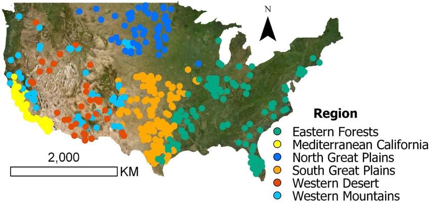
Figure 4. Stacked histograms (a)–(c) and maps (d)–(f) showing Mann–Whitney change test results for (a), (d) annual no-flow
days, (b), (e) days from peak to no-flow, and (c), (f) first no-flow day. Change tests compare the second half of the period of
record (1999–2017) to the first half of the period of record (1980–1998), and units for all plots are days. Only gages with
significant changes (p < 0.05) shown on maps. In all plots, red indicates drier conditions (longer no-flow duration, shorter
dry-down period, earlier first no-flow day) and blue indicates wetter conditions.
8Environ. Res. Lett. 16 (2021) 084033 S C Zipper et al
P/PET trend. Since the PET product we used is cal-
culated using the ASCE Penman–Monteith approach
(Abatzoglou 2013), increases in PET may be driven
by a variety of factors including increases in the vapor
pressure deficit associated with warmer temperatures,
increased turbulent transport due to greater wind
speed, and/or greater incoming solar radiation. Fur-
thermore, our analysis does not measure potential
changes in the timing of P and PET within the year,
apart from the inclusion of seasonal indicators as part
of our random forest analysis (table 1).
We used random forest regression models to fur-
ther explore drivers of spatiotemporal variability in
each intermittency signature. These models provided
annual-resolution predictions of no-flow days, days
from peak to no-flow, and the timing of the first
no-flow day for each gage as a function of climate,
land/water use, and physiography within the contrib-
uting watershed. Model performance, evaluated using
independent test data not used for model develop-
ment (see Materials and Methods section), was strong
for all intermittency signatures and regions (table S2
and figure S12), with the best fit for no-flow duration
(R2 = 0.77, KGE = 0.71), followed by no-flow tim-
ing (R2 = 0.52, KGE = 0.52), and dry-down period
(R2 = 0.35, KGE = 0.39). These performance scores
exceed typical benchmarks for identifying behavioral
hydrological models (KGE > 0.3; Knoben et al 2019)
indicating they are adequate tools to identify the relat-
ive influence of different watershed variables on pre-
dicted intermittency signatures.
The number of annual no-flow days was sensit-
ive to a combination of climatic and physiographic
variables. The most influential predictor variable was
P/PET of the preceding climate year, followed by the
Figure 5. Comparison of Mann-Kendall trends for
(a) annual no-flow days, (b) days from peak to no-flow, gage’s drainage area and P/PET for the current cli-
(c) first no-flow day, against the Mann-Kendall trend mate year (figure 6(a)). By contrast, the dry-down
for the ratio of annual precipitation to potential
evapotranspiration (P/PET). Black line shows a linear best
period was primarily sensitive to land/water use and
fit with 95% confidence interval shaded. Pearson physiography, with wetland cover, drainage area, and
correlations are (a) r = − 0.42, (b) r = 0.05, (c) r = 0.27. forest cover as the most influential predictor vari-
ables (figure 6(b)). Predictions of the no-flow tim-
ing were highly sensitive to climate conditions from
the preceding year. The most influential predictor was
the Mann-Kendall and Mann-Whitney test results P/PET for the preceding climate year, followed by
(figures 3(b) and 4(e)). P/PET for the end of the preceding climate year (Janu-
The importance of changes in P and PET to ary, February, and March) (figure 6(c)). Notably,
P/PET trends varies across regions. In the Northern for both the no-flow duration and timing, preceding
Great Plains, for instance, there is a positive (dry- year climate conditions had a stronger influence on
ing) median PET trend but it is weaker in magnitude annual intermittency signatures than climate condi-
than the positive (wetting) median P trend, and there- tions in the year of interest, indicating that there are
fore the region-wide median P/PET trend indicates time lags between climatic drivers and stream inter-
wetting conditions (figure S4). A similar dynamic mittency response. These time lags suggest that cli-
is present to a lesser degree for the Eastern Forests mate controls on stream intermittency are moderated
region, in which positive trends in P and PET approx- by watershed properties that control the storage and
imately cancel out so that the median P/PET trend is release of water from the landscape, which is further
0. By contrast, the regions in the western US (Western supported by the strong influence of physiographic
Mountains, Western Deserts, Mediterranean Califor- variables such as drainage area, bedrock depth, soil
nia) have both negative P trends and positive PET permeability, and slope in the random forest models
trends, both of which contribute to an overall drying (figure 6). Human impacts are substantial for many
9Environ. Res. Lett. 16 (2021) 084033 S C Zipper et al
Figure 6. Top nine predictor variables for (a) annual no-flow days, (b) days from peak to no-flow, (c) first no-flow day. For
climatic variables, (−1) indicates conditions from the preceding year. The ‘MSE Increase [%]’ is the change in mean squared error
(MSE) when that variable is randomly permuted, expressed as a percentage of overall model MSE, and a higher value is
interpreted as a more important variable. Variable names are defined in table 1.
of the gages in our sample. For instance, 64% of could drive the observed reduction in no-flow condi-
gages are downstream of at least one dam and there is tions.
at least 10% human-modified land use (agricultural The significant changes in stream intermittency
or developed) in the watersheds for more than half we observed during the 1980–2017 period provide
of gages. Despite these widespread human impacts, a multi-decadal window into a long-term traject-
variables associated with human modification of the ory of change. Since our dataset does not include
water cycle (such as irrigation extent, water use, and any hydrologic change that happened prior to 1980,
dam storage; table 1) were not identified as highly our analysis likely underestimates long-term changes
influential predictor variables over any of the inter- in stream intermittency relative to pre-development
mittency signatures. conditions. Irrigation expanded rapidly across much
of CONUS during the 1940–1980 period (Kustu et al
4. Discussion 2010), leading to substantial reductions in peren-
nial stream length prior to 1980 in some regions
4.1. Hydrological change in context (Perkin et al 2017). Looking forward, projected cli-
Our study revealed widespread and primarily dry- mate and land/water use change may lead to fur-
ing trends in stream intermittency across CONUS, ther changes in stream intermittency across much
indicating a temporal and potential spatial expan- of CONUS. For instance, much of the western US
sion of non-perennial flow regimes. Intermittency and Great Plains regions are projected to experi-
trends showed spatial coherence, with most south- ence drier climate throughout the 21st century (Ryu
ern gages demonstrating an increase in no-flow dur- and Hayhoe 2017, Seager et al 2017a, 2017b, Cook
ation, primarily associated with increasing trends in et al 2020), continuing or potentially exacerbating the
aridity (figures 5 and 6). Aridity is a strong pre- observed trend of increasing stream intermittency we
dictor of annual stream intermittency in regional, document in these regions. Given the role of water-
national, and international studies (Jaeger et al 2019, shed storage as a buffer against climate variability, as
Hammond et al 2021, Messager et al 2021, Sauquet evidenced by the importance of physiographic vari-
et al 2021), and here we demonstrate that changes ables in the random forest models (figure 6), cli-
in aridity through time are also contributing to sig- mate change-induced future shifts in stream intermit-
nificant and widespread changes in multiple aspects tency may be most immediately felt in regions with
of stream intermittency. Only a subset of gages loc- relatively little watershed storage (i.e. smaller head-
ated in the Northern Great Plains (15% of gages) water catchments; Costigan et al 2015, Zimmer and
had trends towards fewer annual no-flow days dur- McGlynn 2017) and/or locations with ongoing stor-
ing the period of analysis. The cold-season intermit- age losses (i.e. due to pumping-induced groundwater
tency (Eng et al 2016), decreasing seasonal freezing, and streamflow depletion; Perkin et al 2017, Zipper
and increasing precipitation in the region (figure S4) et al 2019, 2021, Compare et al 2021).
10Environ. Res. Lett. 16 (2021) 084033 S C Zipper et al
Our analysis identified significant and quantifi- with a R2 of 0.77 for no-flow days (table S2) com-
able predictors of no-flow at broad spatial scales. pared to an R2 of ∼0.3 for predictions of no-flow
The clear regional and latitudinal patterns we iden- frequency from Addor et al (2018). We also found
tified (figure 3) contrast with continental-scale work that the different intermittency signatures studied
in Europe that showed little spatial correlation in had diverse drivers, but both annual no-flow days and
stream intermittency trends (Tramblay et al 2021). the timing of no-flow showed a strong dependence
This may be due to greater regional coherence of on antecedent (prior year) climate conditions. The
historical P/PET trends in CONUS (figure S4) com- importance of local factors, such as geology, soil char-
pared to Europe, where regional-scale atmospheric acteristics and river network physiography (Snelder
circulation indicators were not strongly associated et al 2013, Costigan et al 2017, Trancoso et al 2017),
with stream intermittency (Tramblay et al 2021). The indicates that some intermittency signatures (e.g. dry-
regional P/PET trends appear to contribute to the down period) could be harder to predict at large scales
regional trends we observed in the intermittency sig- than others (e.g. no-flow days), perhaps due to the
natures (figures 5 and 6), and in particular climate controls of local surficial geology and perched water
seems to drive the difference in stream intermit- table dynamics on dry-down period (Costigan et al
tency between the northern and southern CONUS. 2015, Zimmer and McGlynn 2018).
By contrast, human activities such as water with-
drawals and dam storage have modest influences on 4.2. Human and environmental implications
nationwide spatiotemporal variability in the inter- Widespread trends towards more intermittent flow
mittency signatures studied here. The lack of signific- in southern CONUS have significant implications
ant human impacts may reflect the fact that anthro- for society and water management. Non-perennial
pogenic disturbances can have a variety of effects streams provide numerous ecosystem services (Datry
that could either increase or decrease stream inter- et al 2018a, Kaletová et al 2019, Stubbington et al
mittency (Gleeson et al 2020), and these impacts 2020) and shifts towards more frequent dry con-
may be more localized and therefore less evident as ditions may enhance some ecosystem services (e.g.
a driver of change in our nationwide analysis. Altern- reducing flood risk by enhancing infiltration capa-
ately, the datasets and variables we used to quantify city; Shanafield and Cook 2014) while decreasing
these activities may not adequately represent their others (e.g. decreasing food production and recre-
potential impact on non-perennial flow regimes. The ation through reduced fish habitat; Perkin et al 2017).
importance of climate as a potential driver of change By contrast, decreased cold-season intermittency in
also corroborates previous work focused on peren- northern CONUS could lead to negative outcomes
nial hydrological signatures. For instance, Ficklin et al such as increased rain-on-snow driven spring flood-
(2018) found widespread climate-driven decreases in ing across the US Midwest (Li et al 2019), while
streamflow in the southern CONUS and increases improving some ecosystem services associated with
in streamflow in the northern CONUS, which were water-related recreation. Effects of changing stream
primarily associated with climate change and present intermittency can also be non-local: the gages exhib-
in both natural and human-impacted watersheds. iting stream intermittency we studied occurred most
Similarly, other work at regional to global scales has often in relatively small headwater catchments (figure
also demonstrated that climate change is the domin- S1), and therefore increasing stream intermittency
ant forcing associated with long-term change in per- could lead to decreases in downstream surface water
ennial hydrological systems, though anthropogenic availability for municipal, industrial, and agricultural
water and land management also have a signific- needs. Ultimately, the implications of these trends for
ant and widespread effect (Rodgers et al 2020, Gud- society will depend on the relative values of compet-
mundsson et al 2021). ing ecosystem services and the degree to which these
Our results provide evidence that no-flow dur- services are replaceable (Datry et al 2018a).
ation, no-flow timing, and dry-down period are The observed widespread trends in no-flow dur-
more predictable than indicated by previous efforts. ation, dry-down period, and no-flow timing also
Although others have found correlations between have diverse and potentially significant implications
stream intermittency and climatic signatures such as for aquatic ecosystems, biogeochemical cycling, and
effective precipitation or aridity at a site to regional water quality. These temporal and spatial trends in
scale (Blyth and Rodda 1973, Jaeger et al 2019, Ward intermittency could inform and refine the biome-
et al 2020, Compare et al 2021), hydrologic sig- specific approach to characterizing freshwater ecosys-
natures related to low-flow and no-flow conditions tem function (Dodds et al 2019), perhaps through the
are among the most challenging to predict at con- more explicit representation of the different stream
tinental scales (Eng et al 2017, Addor et al 2018). drying regimes (Price et al 2021). Intermittency is a
Our random forest models (described in detail in key aspect of stream ‘harshness’ for organisms inhab-
section SI3) compared favorably to previous studies, iting intermittent waters (Fritz and Dodds 2005),
11Environ. Res. Lett. 16 (2021) 084033 S C Zipper et al
and we found that the duration of no-flow signi- 4.3. Monitoring and uncertainty in non-perennial
ficantly increased at 26% of non-perennial gages streams
indicating widespread harsher conditions for aquatic While our analyses revealed widespread trends in
ecosystems. Stream invertebrate communities typic- stream intermittency and investigated watershed-
ally become less biodiverse as the duration of the scale potential drivers, we acknowledge that some
no-flow period increases (Datry et al 2014a), and reach-scale factors could not be resolved (Zimmer
the annual no-flow duration is the most import- et al 2020). While USGS streamflow data under-
ant hydrologic signature in explaining diversity in goes extensive quality assurance before release (Sauer
streams (Leigh and Datry 2017). This suggests that 2002, Sauer and Turnipseed 2010), low flow is partic-
the widespread drying trends we found may be ularly challenging to measure, leading to uncertainty
associated with decreasing biological diversity for associated with stage-discharge relationships and the
most aquatic taxonomic groups. In settings where stage corresponding to no-flow. For example, we are
drying has historically been less common, such as unable to distinguish no-flow conditions where pon-
humid regions, increased drying may trigger shifts ded surface water remains from no-flow readings
to more desiccation-resistant communities (Drum- where the channel is completely dry, despite differ-
mond et al 2015) and therefore these settings may ing ecological, biogeochemical, and societal impacts
experience greater ecological changes in response to of these two conditions (Kaletová et al 2019, Stub-
changes in drying than more arid regions where dry- bington et al 2020). Furthermore, in some settings
ing has been historically common. No-flow dura- there may be subsurface flow that bypasses the stream
tion also affects biogeochemistry and therefore has gage and emerges downstream, particularly where the
potential water quality implications. Longer no-flow subsurface is highly transmissive (Costigan et al 2015,
duration has been found elsewhere to contribute Zimmer et al 2020). Since some of our gages are
to decreased gross primary productivity (Colls et al within the same watershed, there may be correlated
2019), increased ammonia oxidation activity, and intermittency dynamics that propagate up- or down-
increased sediment nitrate content (Merbt et al 2016). stream within a watershed. We found that poten-
Therefore, regionally distinct shifts in ecological and tial redundancy among gages within the same water-
biogeochemical processes may be associated with shed did not impact our results or conclusions (sup-
longer/shorter no-flow duration in southern/north- plemental information, section SI4), and therefore
ern CONUS, respectively. our results provide the most complete possible pic-
We also observed trends for a shorter dry-down ture of changing intermittency over CONUS given the
period and an earlier no-flow timing for 10% of the current distribution of gaged non-perennial streams
streams investigated. Drying rate acts as an import- (figure 1).
ant environmental cue for stream invertebrate com- Considering these uncertainties, our study high-
munities (Drummond et al 2015), and the no-flow lights the critical need for adequate non-perennial
timing controls habitat connectivity during critical stream gage coverage in the US hydrometric net-
spring spawning periods for fish in non-perennial work by documenting stream intermittency trends
river networks (Jaeger et al 2014). While some spe- across large portions of CONUS. Typically, river gages
cies have adapted to migrate to perennial reaches are installed to support human-oriented water needs,
as flow rates decline (Lytle et al 2008), more rapid including allocation of water resources, flood haz-
drying could disrupt such responses (Robson et al ard mitigation, and riverine navigation (Ruhi et al
2011). Furthermore, spring is the high-flow season in 2018). Because of this priority in gage placement,
the southwestern US where we observed widespread stream reaches that experience low-flow conditions
trends towards earlier no-flow conditions (figures 1 are underrepresented in gage networks, with wide
and 4). Earlier drying during this period may decrease swaths of the CONUS that do not have any long-term
primary productivity, which is often greatest in spring gaging on non-perennial streams (Zimmer et al 2020)
prior to leaf-out of riparian ecosystems (Myrstener (figure 1(a)). Thus, our analysis paints an incom-
et al 2021), while concurrently enhancing leaf litter plete and potentially conservative picture of chan-
decomposition within streams (Gonçalves et al 2019). ging stream intermittency across CONUS. Our find-
Given the widespread changes in stream intermit- ings illustrate clear regional patterns in intermittency
tency and associated societal, ecological, and biogeo- despite the relatively low coverage of non-perennial
chemical implications of these changes, water man- streams in the existing US gage network. Place-
agement and policy around non-perennial streams ment of additional gages in non-perennial streams
needs to be responsive not just to whether a stream is in a variety of ecoregions would improve our abil-
non-perennial or not, but also the regional patterns ity to understand drivers of change and inform
and drivers of changes in duration, timing, and dry- management and policy related to non-perennial
down period. streams.
12Environ. Res. Lett. 16 (2021) 084033 S C Zipper et al
4.4. Policy and management of non-perennial characteristics. Changes in no-flow duration and
streams especially timing are primarily driven by climate,
Recent U.S. policy debate has centered on the ques- while land/water use and physiography have a larger
tion of whether waters that dry on a regular basis— influence over the dry-down period. Human activities
non-perennial streams and wetlands—are sufficiently such as reservoirs or water use did not show up as sig-
critical to the integrity of downstream perennial nificant drivers of variability for any of the intermit-
waters that they should receive the same federal pro- tency signatures. This indicates that watershed-scale
tections (Alexander et al 2018, Sills et al 2018, Walsh management interventions may struggle to modify
and Ward 2019, Sullivan et al 2020). The Rapanos v. the timing, duration, or dry-down period of no-
US (2006) Supreme Court decision addressed which flow, which are more strongly driven by regional to
waters would receive federal protections under the global climate change. The changes we document are
Clean Water Act and urged regulatory agencies to likely to have substantial ecological, biogeochemical,
issue clear guidance. In response, the US EPA pro- and societal implications and their consideration will
mulgated the Clean Water Rule (2015), which was improve watershed management and policy.
then repealed and replaced by the Navigable Waters
Protection Rule (2020), and is currently (as of 2021) Data availability statement
under further review. Our finding that stream inter-
mittency is changing over much of CONUS leads to Data and code associated with this study are
the conclusion that binary classifications into ‘per- available in the HydroShare repository: https:/
ennial’, ‘intermittent’, and ‘ephemeral’ used in these /doi.org/10.4211/hs.fe9d240438914634abbfd-
US policies may not be valid as non-perennial flow cfa03bed863.
dynamics can change through time. Given the pre-
dictable drivers of flow intermittency we identify,
the time period over which these classifications are Acknowledgments
determined should faithfully reflect the mechanisms
driving local intermittency, such as climate change. In This manuscript is a product of the Dry Rivers
addition, the regional nature of change we observed Research Coordination Network, which was suppor-
(figure 4) and the degree to which stream inter- ted by funding from the US National Science Found-
mittency is predictable based on climate, land/wa- ation (DEB-1754389). Any use of trade, firm, or
ter use, and physiography (figure 6) hints that future product names is for descriptive purposes only and
policy may be able to target different aspects of non- does not imply endorsement by the US Govern-
perennial flow for improved management. Our work ment. This manuscript was improved by construct-
here is one possible basis for assessing flow frequency ive feedback from Kristin Jaeger and three anonym-
to determine the jurisdictional status of a river or ous reviews.
stream, consistent with the procedures set forth in
the Navigable Waters Protection Rule. Critically, fur- ORCID iDs
ther work is needed to understand how the hydrolo-
gic change we document here may cascade to impact Samuel C Zipper https://orcid.org/0000-0002-
physical, chemical, and biological functions of both 8735-5757
non-perennial streams and downstream perennial C Nathan Jones https://orcid.org/0000-0002-
water bodies, and to understand the broader implic- 5804-0510
ations of changing stream intermittency for society. Michelle H Busch https://orcid.org/0000-0003-
4536-3000
5. Conclusions Adam N Price https://orcid.org/0000-0002-7211-
4758
Our study revealed dramatic and widespread changes George H Allen https://orcid.org/0000-0001-
in stream intermittency across CONUS. Half of the 8301-5301
non-perennial gage network has experienced a signi- Corey A Krabbenhoft https://orcid.org/0000-
ficant change in the no-flow duration, no-flow tim- 0002-2630-8287
ing, and/or dry-down period over the past 40 years,
with distinct regional patterns. Streams are experien- References
cing longer no-flow conditions and an earlier onset
Abatzoglou J T 2013 Development of gridded surface
of no-flow in the southern CONUS, while the oppos-
meteorological data for ecological applications and
ite is true in the northern CONUS. By contrast, modelling Int. J. Climatol. 33 121–31
changes in the dry-down period are less prevalent Acuña V, Datry T, Marshall J, Barceló D, Dahm C N, Ginebreda A,
and less spatially consistent. We developed predictive McGregor G, Sabater S, Tockner K and Palmer M A 2014
Why should we care about temporary waterways? Science
models for these intermittency signatures and found
343 1080–1
that spatiotemporal variability is driven by a mix- Addor N, Nearing G, Prieto C, Newman A J, Vine N L and
ture of climate, land/water use, and physiographic Clark M P 2018 A ranking of hydrological signatures based
13Environ. Res. Lett. 16 (2021) 084033 S C Zipper et al
on their predictability in space Water Resour. Res. Dodds W K and Oakes R M 2008 Headwater influences on
54 8792–812 downstream water quality Environ. Manage. 41 367–77
Alexander L C et al 2018 Featured collection introduction: Drummond L R, McIntosh A R and Larned S T 2015 Invertebrate
connectivity of streams and wetlands to downstream waters community dynamics and insect emergence in
JAWRA 54 287–97 response to pool drying in a temporary river Freshw. Biol.
Allen D C et al 2020 River ecosystem conceptual models and 60 1596–612
non-perennial rivers: a critical review WIREs Water 7 e1473 Dudley R W, Hirsch R M, Archfield S A, Blum A G and Renard B
Allen D C, Kopp D A, Costigan K H, Datry T, Hugueny B, 2020 Low streamflow trends at human-impacted and
Turner D S, Bodner G S and Flood T J 2019 Citizen scientists reference basins in the United States J. Hydrol.
document long-term streamflow declines in intermittent 580 124254
rivers of the desert southwest, USA Freshw. Sci. 38 244–56 Eng K, Grantham T E, Carlisle D M and Wolock D M 2017
Beaufort A, Lamouroux N, Pella H, Datry T and Sauquet E 2018 Predictability and selection of hydrologic metrics in riverine
Extrapolating regional probability of drying of headwater ecohydrology Freshw. Sci. 36 915–26
streams using discrete observations and gauging networks Eng K, Wolock D M and Dettinger M D 2016 Sensitivity of
Hydrol. Earth Syst. Sci. 22 3033–51 intermittent streams to climate variations in the USA River
Blyth K and Rodda J C 1973 A stream length study Water Resour. Res. Appl. 32 885–95
Res. 9 1454–61 Falcone J A 2011 GAGES-II: Geospatial Attributes of Gages for
Breiman L 2001 Random forests Mach. Learn. 45 5–32 Evaluating Streamflow (Reston, VA: U.S. Geological Survey)
Broxton P, Zeng X and Dawson N 2019 Daily 4 km gridded SWE Falcone J A 2016 County fresh-water withdrawal water use
and snow depth from assimilated in-situ and modeled data allocated to relevant land uses in the United States:
over the conterminous US, version 1 (available at: https:// 1985–2010 (U.S. Geological Survey data release) (https://
nsidc.org/data/nsidc-0719/versions/1) (Accessed 22 January doi.org/10.5066/F7DJ5CR)
2021) Falcone J A 2017 U.S. Geological Survey GAGES-II time series
Busch M H et al 2020 What’s in a name? Patterns, trends, and data from consistent sources of land use, water use,
suggestions for defining non-perennial rivers and streams agriculture, timber activities, dam removals, and other
Water 12 1980 historical anthropogenic influences (https://doi.org/
Colls M, Timoner X, Font C, Sabater S and Acuña V 2019 Effects 10.5066/F7HQ3XS4)
of duration, frequency, and severity of the non-flow period Ficklin D L, Abatzoglou J T, Robeson S M, Null S E and
on stream biofilm metabolism Ecosystems 22 1393–405 Knouft J H 2018 Natural and managed watersheds show
Compare K, Zipper S C, Zhang C and Seybold E 2021 similar responses to recent climate change Proc. Natl Acad.
Characterizing streamflow intermittency and subsurface Sci. 115 8553–57
heterogeneity in the middle Arkansas river basin Kansas Fritz K M and Dodds W K 2005 Harshness: characterisation of
Geological Survey Open-File Report 2021–1 (Lawrence KS) intermittent stream habitat over space and time Mar. Freshw.
(available at: www.kgs.ku.edu/Publications/OFR/2021/ Res. 56 13
OFR2021-1.pdf) (Accessed 13 May 2021) Fry J A, Xian G, Jin S M, Dewitz J A, Homer C G, Yang L M,
Cook B I, Mankin J S, Marvel K, Williams A P, Smerdon J E and Barnes C A, Herold N D and Wickham J D 2011
Anchukaitis K J 2020 Twenty-first century drought Completion of the 2006 national land cover database for the
projections in the CMIP6 forcing scenarios Earth’s Future conterminous United States PE&RS Photogramm. Eng.
8 e2019EF001461 Remote Sens. 77 858–64
Costigan K H, Daniels M D and Dodds W K 2015 Fundamental Gleeson T et al 2020 Illuminating water cycle modifications and
spatial and temporal disconnections in the hydrology of an Earth system resilience in the Anthropocene Water Resour.
intermittent prairie headwater network J. Hydrol. Res. 56 e2019WR024957
522 305–16 Gleeson T, Moosdorf N, Hartmann J and Van Beek L P H 2014 A
Costigan K H, Kennard M J, Leigh C, Sauquet E, Datry T and glimpse beneath earth’s surface: gLobal HYdrogeology MaPS
Boulton A J 2017 Chapter 2.2—Flow regimes in intermittent (GLHYMPS) of permeability and porosity Geophys. Res.
rivers and ephemeral streams Intermittent Rivers and Lett. 41 2014GL059856
Ephemeral Streams T Datry ed N Bonada and A Boulton Gómez-Gener L, Lupon A, Laudon H and Sponseller R A 2020
(New York: Academic) pp 51–78 Drought alters the biogeochemistry of boreal stream
Cudennec C, Leduc C and Koutsoyiannis D 2007 Dryland networks Nat. Commun. 11 1795
hydrology in Mediterranean regions—a review Hydrol. Sci. Gonçalves A L, Simões S, Bärlocher F and Canhoto C 2019 Leaf
J. 52 1077–87 litter microbial decomposition in salinized streams under
Datry T et al 2018b A global analysis of terrestrial plant litter intermittency Sci. Total Environ. 653 1204–12
dynamics in non-perennial waterways Nat. Geosci. Gudmundsson L et al 2021 Globally observed trends in mean and
11 497–503 extreme river flow attributed to climate change Science
Datry T, Boulton A J, Bonada N, Fritz K, Leigh C, Sauquet E, 371 1159–62
Tockner K, Hugueny B and Dahm C N 2018a Flow Gupta H V, Kling H, Yilmaz K K and Martinez G F 2009
intermittence and ecosystem services in rivers of the Decomposition of the mean squared error and NSE
Anthropocene J. Appl. Ecol. 55 353–64 performance criteria: implications for improving
Datry T, Larned S T, Fritz K M, Bogan M T, Wood P J, Meyer E I hydrological modelling J. Hydrol. 377 80–91
and Santos A N 2014a Broad-scale patterns of invertebrate Hammond J C et al 2021 Spatial patterns and drivers of
richness and community composition in temporary rivers: nonperennial flow regimes in the contiguous United States
effects of flow intermittence Ecography 37 94–104 Geophys. Res. Lett. 48 e2020GL090794
Datry T, Larned S T and Klement T 2014b Intermittent rivers: Hengl T et al 2017 SoilGrids250m: global gridded soil
a challenge for freshwater ecology BioScience information based on machine learning PloS One
64 229–35 12 e0169748
Datry T, Pella H, Leigh C, Bonada N and Hugueny B 2016 A Homer C, Dewitz J, Fry J, Coan M, Hossain N, Larson C,
landscape approach to advance intermittent river ecology Herold N, McKerrow A, VanDriel J N and Wickham J 2007
Freshw. Biol. 61 1200–13 Completion of the 2001 national land cover database for the
Dodds W K, Bruckerhoff L, Batzer D, Schechner A, Pennock C, conterminous United States Photogramm. Eng. Remote Sens.
Renner E, Tromboni F, Bigham K and Grieger S 2019 The 73 5
freshwater biome gradient framework: predicting Homer C, Dewitz J, Yang L, Jin S, Danielson P, Xian G, Coulston J,
macroscale properties based on latitude, altitude, and Herold N, Wickham J and Megown K 2015 Completion of
precipitation Ecosphere 10 e02786 the 2011 national land cover database for the conterminous
14You can also read