Assessment of precipitation error propagation in multi-model global water resource reanalysis - HESS
←
→
Page content transcription
If your browser does not render page correctly, please read the page content below
Hydrol. Earth Syst. Sci., 23, 1973–1994, 2019
https://doi.org/10.5194/hess-23-1973-2019
© Author(s) 2019. This work is distributed under
the Creative Commons Attribution 4.0 License.

Assessment of precipitation error propagation in multi-model global
water resource reanalysis
Md Abul Ehsan Bhuiyan1 , Efthymios I. Nikolopoulos1 , Emmanouil N. Anagnostou1 , Jan Polcher2 , Clément Albergel3 ,
Emanuel Dutra4 , Gabriel Fink5 , Alberto Martínez-de la Torre6 , and Simon Munier3
1 Department  of Civil and Environmental Engineering, University of Connecticut, Storrs, CT, USA
2 Laboratoire de Météorologie Dynamique du CNRS/IPSL, École Polytechnique, Paris, France
3 CNRM-Université de Toulouse, Météo-France, CNRS, 31057 Toulouse, France
4 Instituto Dom Luiz, Faculdade de Ciências, Universidade de Lisboa, Lisbon, Portugal
5 Landesanstalt für Umwelt Baden-Württemberg (LUBW), Karlsruhe, Germany
6 Centre for Ecology and Hydrology, Wallingford, UK

Correspondence: Emmanouil N. Anagnostou (manos@uconn.edu)

Received: 10 August 2018 – Discussion started: 1 October 2018
Revised: 15 February 2019 – Accepted: 15 March 2019 – Published: 15 April 2019

Abstract. This study focuses on the Iberian Peninsula and        schemes and show that uncertainties in the model simula-
investigates the propagation of precipitation uncertainty, and   tions are attributed to both uncertainty in precipitation forc-
its interaction with hydrologic modeling, in global water re-    ing and the model structure. Surface runoff is strongly sen-
source reanalysis. Analysis is based on ensemble hydrologic      sitive to precipitation uncertainty, and the degree of sensitiv-
simulations for a period spanning 11 years (2000–2010). To       ity depends significantly on the runoff generation scheme of
simulate the hydrological variables of surface runoff, sub-      each model examined. Evapotranspiration fluxes are compar-
surface runoff, and evapotranspiration, we used four land        atively less sensitive for this study region. Finally, our results
surface models (LSMs) – JULES (Joint UK Land Environ-            suggest that there is no single model–forcing combination
ment Simulator), ORCHIDEE (Organising Carbon and Hy-             that can outperform all others consistently for all variables
drology In Dynamic Ecosystems), SURFEX (Surface Exter-           examined and thus reinforce the fact that there are signifi-
nalisée), and HTESSEL (Hydrology – Tiled European Centre         cant benefits to exploring different model structures as part
for Medium-Range Weather Forecasts – ECMWF – Scheme              of the overall modeling approaches used for water resource
for Surface Exchanges over Land) – and one global hydro-         applications.
logical model, WaterGAP3 (Water – a Global Assessment
and Prognosis). Simulations were carried out for five precip-
itation products – CMORPH (the Climate Prediction Cen-
ter Morphing technique of the National Oceanic and Atmo-         1   Introduction
spheric Administration, or NOAA), PERSIANN (Precipita-
tion Estimation from Remotely Sensed Information using           Improved estimation of global precipitation is important to
Artificial Neural Networks), 3B42V(7), ECMWF reanalysis,         the analysis of continental water resources and dynamics.
and a machine-learning-based blended product. As a refer-        Over the past few decades, several studies have described the
ence, we used a ground-based observation-driven precipita-       use of different precipitation algorithms to develop precip-
tion dataset, named SAFRAN, available at 5 km, 1 h reso-         itation products (http://ipwg.isac.cnr.it/algorithms.html, last
lution. We present relative performances of hydrologic vari-     access: 31 March 2019 and http://reanalyses.org, last access:
ables for the different multi-model and multi-forcing scenar-    31 March 2019) at high spatial and temporal resolution on
ios. Overall, results reveal the complexity of the interaction   a quasi-global scale and for different hydrological applica-
between precipitation characteristics and different modeling     tions, such as flood early warning and control and drought
                                                                 monitoring (Hong et al., 2010; Wu et al., 2012; Vernimmen

Published by Copernicus Publications on behalf of the European Geosciences Union.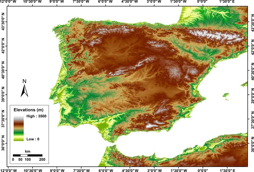
1974 M. A. Ehsan Bhuiyan et al.: Multi-parameter water resource reanalysis uncertainty characterization
et al., 2012, amongst others). Precipitation estimates suffer, ment and planning. This additionally means that there is also
however, from various sources of error that consequently a need to assess hydrologic uncertainty in more than a single
impact hydrologic investigations (Mei et al., 2015, 2016; variable to be able to have a better and more integrative view
Seyyedi et al., 2014, 2015; Bhuiyan et al., 2017; Nikolopou- on the interaction between forcing uncertainty, model uncer-
los et al., 2013). tainty, and the hydrologic variable of interest. It will allow
Over the last decade, an increasing number of studies have us to make hydrologic predictions more effective for water
contributed to the development of global precipitation esti- resource applications at a large scale.
mation (Pan et al., 2010; Beck et al., 2017a; Kirstetter et al., This study builds upon a unique numerical experiment that
2014; Carr et al., 2015; Dee et al., 2011) aiming at the over- was carried out, as part of the activities of the Earth2Observe
all improvement of the hydrological applications and global project (Schellekens et al., 2017), to investigate the impact of
water resource reanalysis. Numerous models of varying com- precipitation uncertainty propagation and its dependence on
plexity can be used to generate an array of hydrological prod- model structure and hydrologic variables. In this investiga-
ucts from precipitation forcing datasets (Vivoni et al., 2007; tion, we used different precipitation forcing datasets based
Ogden and Julien, 1994; Carpenter et al., 2001; Borga, 2002; on (i) reanalysis, (ii) satellite estimates, and (iii) a “com-
Schellekens et al., 2017). Different hydrological models have bined” stochastic precipitation dataset (Bhuiyan et al., 2018).
different applications depending on the spatial and temporal To consider model structure and parameters, we examined
scales of interest as well as the simulated variables of interest, simulations from five state-of-the-art global-scale hydrolog-
such as subsurface runoff, surface runoff, and evapotranspi- ical and land surface models (LSMs). With regard to water
ration. Past studies (Fekete et al., 2004; Biemans et al., 2009) cycle variables, we evaluated precipitation uncertainty prop-
have revealed that the uncertainty in simulated hydrological agation to surface runoff, subsurface runoff, and evapotran-
variables mainly depends on the uncertainty in precipitation spiration fluxes. The study area for this investigation is the
and model parametrization and suggested subsequent explo- Iberian Peninsula, which has precipitation and climate vari-
ration of different model structures as part of the overall mod- ability due to complex orography influenced by both Atlantic
eling approach. and Mediterranean climates (Rodríguez-Puebla et al., 2001;
So far there are several studies that have analyzed un- de Luis et al., 2010; Herrera et al., 2012). The analysis com-
certainty in precipitation forcing and its impact on hydro- prised two main parts: (1) performance and sensitivity eval-
logic simulations by usually evaluating hydrologic simula- uation of the different model–forcing scenarios and (2) pre-
tions based on multiple forcing applied to a single model cipitation uncertainty propagation to the hydrological vari-
(Falck et al., 2015; Bitew et al., 2012; Behrangi et al., 2011; ables. We analyzed hydrological simulation with a compara-
Mei et al., 2016; Bhuiyan et al., 2018; Gelati et al., 2018 tive assessment of the hydrological products and provided a
among others). On the other hand, there are also past studies detailed analysis of uncertainty in hydrological simulations
that have evaluated the model structural uncertainty and its for the different global hydrological and land surface mod-
impact on hydrologic simulations, usually by analyzing the els used in the multi-model global water resource reanalysis.
simulation outputs from multiple models and a single forc- Finally, we examined the performance of precipitation prod-
ing dataset (Breuer et al., 2009; Haddeland et al., 2011; Gud- ucts in hydrological applications and potential uncertainty at-
mundsson et al., 2012; Smith et al., 2013; Huang et al., 2017; tributed to precipitation error propagations.
Beck et al., 2017b). However, fewer studies have been dedi- The paper is structured as follows. Section 2 presents the
cated to the analysis of the integrated impact of both forcing different types of forcing datasets used for the study, and
and model uncertainty on hydrologic simulations, and from Sect. 3 details the methodology we used for our model de-
the existing ones, most of them were focused on a single hy- velopment and hydrological model analysis. Section 4 sum-
drologic variable such as streamflow (see, for example, Qi marizes the hydrological results, Sect. 5 discusses the results,
et al. 2016), evapotranspiration (Vinukollu et al., 2011), or and Sect. 6 draws conclusions from the research conducted.
a given hydrologic index such as the drought index (Prud-
homme et al., 2014; Samaniego et al., 2017). Findings from
these past investigations have demonstrated that both forc- 2 Study area and forcing data
ing and model structure uncertainty have a great impact on
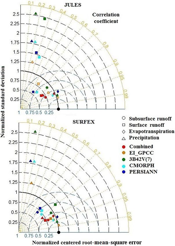
This study is focused on the Iberian Peninsula (Fig. 1). The
hydrologic predictions and therefore highlight that using a
climate of the peninsula is primarily Mediterranean, being
multi-model and multi-forcing ensemble is a more appropri-
mostly oceanic at northern and semi-arid at southern parts.
ate path forward for advancing the use of hydrologic model
The topography varies from almost zero elevation to altitudes
outputs. This conclusion raises at the same time the need for
of 3500 m in the Pyrenees. Table 1 summarizes information
better understanding, characterizing and quantifying the un-
and references of meteorological forcing datasets, and a short
certainty associated with multi-model and multi-forcing hy-
description is provided below.
drologic ensembles. Thus, a better understanding of the en-
semble spread of precipitation and simulated hydrological
variables is necessary to improve water resource manage-
Hydrol. Earth Syst. Sci., 23, 1973–1994, 2019 www.hydrol-earth-syst-sci.net/23/1973/2019/
M. A. Ehsan Bhuiyan et al.: Multi-parameter water resource reanalysis uncertainty characterization                          1975

2.1   Reference precipitation (SAFRAN)                             with a multiplicative factor to match GPCC version 7 for
                                                                   the period 1979–2013 and GPCC monitoring for 2013–2015.
The reference precipitation dataset, hereafter referred to as      Data are further downscaled to 0.25◦ × 0.25◦ grid resolu-
SAFRAN (Système d’analyse fournissant des renseigne-               tion by distributing the coarse grid precipitation according
ments atmosphériques à la neige), was recently created by          to CHPclim (Climate Hazards Group Precipitation Climatol-
Quintana-Seguí et al. (2016, 2017) using the SAFRAN me-            ogy) high-resolution information for each calendar month. A
teorological analysis system (Durand et al., 1993). Spa-           similar approach was performed in the generation of ERA-
tially, SAFRAN precipitation data are presented at an hourly       Interim/Land (Balsamo et al., 2015), but using GPCP (Global
timescale on a regular grid with 5 km resolution, spanning         Precipitation Climatology Project) data. In this study we used
35 years and covering mainland Spain, Portugal, and the            GPCC data due to its higher spatial resolution when com-
Balearic Islands (Quintana-Seguí et al., 2016). SAFRAN             pared with GPCP.
used an optimal interpolation algorithm (Gandin, 1966) to
produce a quality-controlled gridded dataset of precipitation      2.4    Combined product
which combines ground observations and outputs of a me-
teorological model (Quintana-Seguí et al., 2017). Quintana-        The combined product is based on the application of
Seguí et al. (2017) also compared the different precipita-         a nonparametric statistical technique for blending multi-
tion analyses with rain gauge data and successfully evalu-         ple satellite–reanalysis precipitation datasets. Specifically,
ated their temporal and spatial similarities to the observations   a machine-learning technique, quantile regression forests
by obtaining higher correlation ( > 0.75) than other precip-       (QRF; Meinshausen, 2006), was used to generate stochasti-
itation products. The validation of SAFRAN with indepen-           cally an improved precipitation ensemble at the spatiotempo-
dent ground observations proved that SAFRAN is a robust            ral resolution of 0.25◦ , 3 h. The technique optimally merged
product. On the other hand, several factors – including rain-      global precipitation datasets and characterized the uncer-
fall intermittency, discrete temporal sampling, and censoring      tainty of the combined product. Details on the methodology
of reference values for required quality – reduce the number       and data used to develop the combined product are presented
of comparison samples for reference and satellite estimates.       in Bhuiyan et al. (2018).
Therefore, the quality-controlled SAFRAN dataset which is
designed to force the land surface model is chosen as a refer-     2.5    Other atmospheric variables
ence dataset for the study area (Quintana-Seguí et al., 2017).
                                                                   Apart from precipitation forcing, the rest of atmospheric
                                                                   forcing variables required for the hydrologic simulations
2.2   Satellite-based precipitation
                                                                   were derived from the original ERA-Interim 3-hourly data as
                                                                   used in ERA-Interim/Land (Balsamo et al., 2015), bilinearly
Satellite-based simulations were based on three quasi-global
                                                                   interpolated to 0.25◦ . It includes a topographic adjustment to
satellite precipitation products. Among them, CMORPH (the
                                                                   temperature, humidity, and pressure using a spatially tempo-
Climate Prediction Center Morphing technique of the Na-
                                                                   rally varying environmental lapse rate (ELR) computed sim-
tional Oceanic and Atmospheric Administration, or NOAA)
                                                                   ilarly to Gao et al. (2012). The correction is the following:
is developed from passive microwave (PMW) satellite pre-
                                                                   (i) relative humidity is computed from the uncorrected forc-
cipitation fields which are generated from motion vectors de-
                                                                   ing, (ii) air temperature is corrected using the ELR and al-
rived from infrared (IR) data (Joyce et al., 2004). A neural
                                                                   titude differences (ERA-Interim topography versus 0.25 to-
network technique is used in PERSIANN (Precipitation Es-
                                                                   pography), (iii) surface pressure is corrected assuming the
timation from Remotely Sensed Information using Artificial
                                                                   altitude difference and updated temperature, and (iv) specific
Neural Networks), where IR observations are connected to
                                                                   humidity is computed using the new surface pressure and
PMW rainfall estimates (Sorooshian et al., 2000). Merged
                                                                   temperature assuming no changes in relative humidity.
IR and PMW precipitation products from NASA are gauge-
adjusted for TMPA (Tropical Rainfall Measuring Mission
Multi-Satellite Precipitation Analysis), or 3B42V(7), which        3     Methodology
is available in near-real time and post-real time (Huffman et
al., 2010). The satellite precipitation products have a spatial    3.1    Hydrological simulations
resolution that is 0.25◦ × 0.25◦ and a time resolution of 3 h.
                                                                   The hydrological simulations for this study were carried
2.3   Atmospheric reanalysis                                       out by different collaborators within the framework of
                                                                   Earth2Observe, a project funded by the European Union
The reanalysis product (EI_GPCC) is based on original              (EU) using a number of global-scale land surface and hy-
ERA-Interim 3-hourly data, after rescaling based on GPCC           drological models. In this study, simulations from four land
(Global Precipitation Climatology Center) data. Note that          surface models – JULES (Joint UK Land Environment Sim-
total precipitation has been rescaled at the monthly scale         ulator), ORCHIDEE (Organising Carbon and Hydrology

www.hydrol-earth-syst-sci.net/23/1973/2019/                                     Hydrol. Earth Syst. Sci., 23, 1973–1994, 2019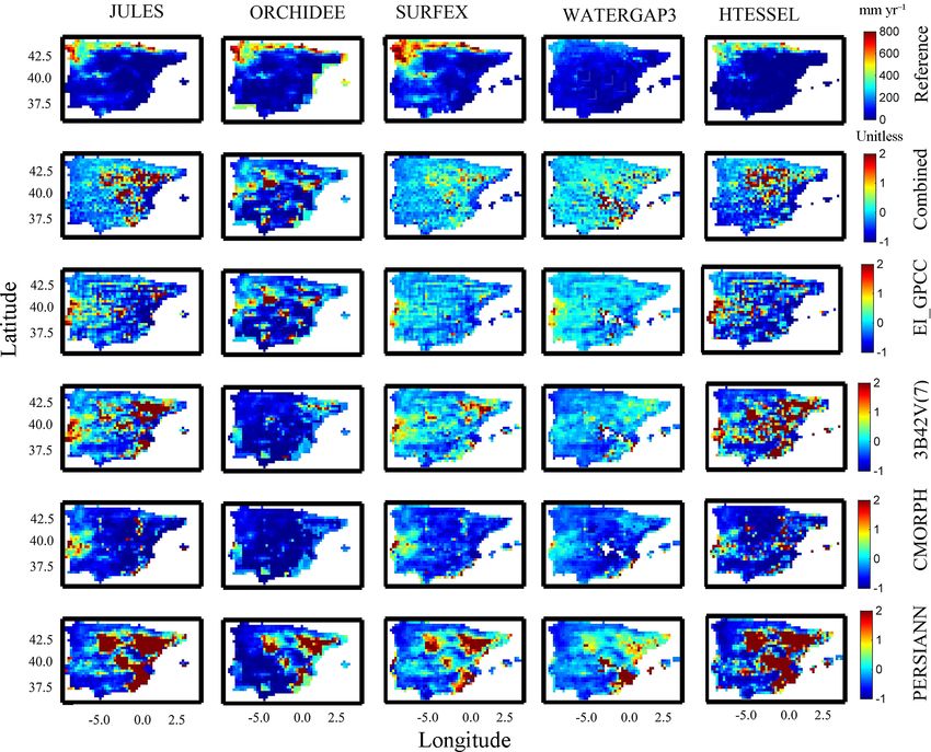
1976                M. A. Ehsan Bhuiyan et al.: Multi-parameter water resource reanalysis uncertainty characterization

Figure 1. Map of Iberian Peninsula case study area.

In Dynamic Ecosystems), SURFEX (Surface Externalisée),             the surface is divided into infiltration into the soil and sur-
and HTESSEL (Hydrology – Tiled European Centre for                 face runoff. Surface runoff is generated either through infil-
Medium-Range Weather Forecasts – ECMWF – Scheme for                tration excess or saturation excess. Infiltration excess runoff
Surface Exchanges over Land) – and one global hydrologi-           is generated by JULES if the water flux reaching the surface
cal model, the distributed global hydrological model of the        exceeds the maximum infiltration rate of the soil (based on
WaterGAP3 (Water – a Global Assessment and Prognosis)              the saturated hydraulic conductivity). If the water flux reach-
modeling framework were considered. The models were al-            ing the surface over a time step (either rainfall, throughfall,
ready evaluated at all timescales, from daily to multi-annual.     or snowmelt) reaches a maximal infiltration rate, then infil-
The timescale of the evaluation was mostly driven by the data      tration excess runoff will be generated. This maximal infil-
availability. All the land surface models in the study were        tration rate in JULES is the saturated hydraulic conductiv-
global models, built originally to work in coupled mode with       ity multiplied by a vegetation-dependent parameter (four for
atmospheric models. The “regionalization”, or calibration of       trees and two for grasses). Saturation excess runoff is based
hydrological parameters at particular catchments or regions        on sub-grid soil moisture variability, as a fraction of the grid
of these models, is an exercise that the different modeling        is saturated and water flux over this fraction is converted to
groups or communities are certainly performing but was out         surface runoff (probability distribution model; Blyth, 2002).
of the scope of this study. All models were forced with the        Once infiltrated into the soil, water flows through the column,
various precipitation datasets described in the previous sec-      resolved using Darcy’s law and Richards’ equation. Subsur-
tion for an 11-year period (March 2000–December 2010). A           face runoff is calculated using the free drainage approach,
summary of some basic characteristics of the models struc-         with water flowing at the bottom of the resolved soil column
ture is presented in Table 1 and a short description is pro-       at a rate determined by the soil hydraulic conductivity. There
vided below. For more details on the modeling systems, the         was no groundwater table in this version of JULES. The con-
interested reader is referred to Schellekens et al. (2017) and     dition at the bottom of the resolved soil layers (3 m) was
references therein.                                                assumed to be free drainage. The soil hydraulic character-
                                                                   istics were calculated applying pedotransfer functions to the
3.1.1   JULES                                                      soil texture data from the Harmonized World Soil Database
                                                                   (HWSD; FAO/IIASA/ISRIC/ISS-CAS/JRC, 2012).The veg-
JULES (Best et al., 2011; Clark et al., 2011) is a physically      etation cover data used by the JULES runs were derived
based land surface model. JULES uses an exponential rain-          from the International Geosphere-Biosphere Programme at
fall intensity distribution to calculate throughfall through the   http://www.igbp.net/ (last access: 31 March 2019). Further
canopy first (altered by interception), then the water reaching

Hydrol. Earth Syst. Sci., 23, 1973–1994, 2019                                    www.hydrol-earth-syst-sci.net/23/1973/2019/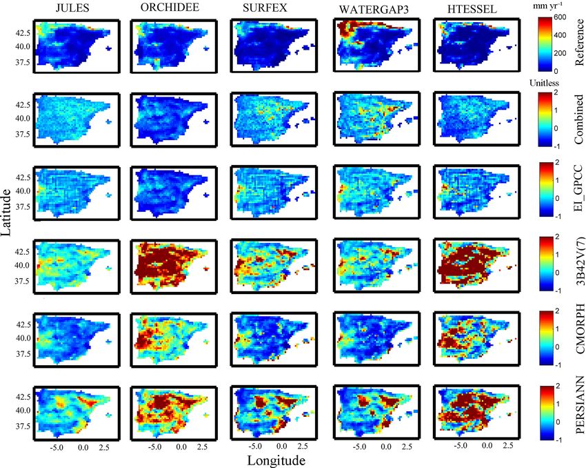
M. A. Ehsan Bhuiyan et al.: Multi-parameter water resource reanalysis uncertainty characterization                              1977

details on hydrology processes in JULES can be found in             3.1.4   WATERGAP3
Best et al. (2011) and Blyth et al. (2018).
                                                                    The modeling framework WaterGAP3 is a tool for assessing
3.1.2   ORCHIDEE                                                    the global freshwater resources on 30 min spatial resolution.
                                                                    It combines a spatially distributed rainfall–runoff model with
ORCHIDEE (Krinner et al., 2005) is a complex land sur-              a large-scale water quality model as well as models for five
face scheme that consists of a hydrological module, a rout-         sectorial water uses (Flörke et al., 2013; Döll et al., 2009).
ing module (Ngo-Duc et al., 2007), and a floodplain module          Effective precipitation – calculated as superposed effects of
(d’Orgeval et al., 2008). It also describes the vegetation dy-      snow accumulation, snowmelt, and interception – is split into
namics and biological cycles, but these features were not ac-       (i) a fraction that fills up a single-layer soil moisture storage
tivated for the present study. The most relevant parametriza-       and (ii) a fraction that comprises surface runoff and ground-
tion of ORCHIDEE for the sensitivity of the model to rain-          water recharge. Groundwater recharge is the input of a sin-
fall is the one for partitioning between infiltration and sur-      gle linear groundwater reservoir that is drained by base flow.
face runoff. In order to represent correctly the fast progres-      Water for evapotranspiration, estimated with the Priestley–
sion of the moisture front during a rainfall event when the         Taylor approach, is abstracted from the soil storage. The Wa-
time step is above 15 min, a time-splitting procedure is used       terGAP3 setting used in this study was calibrated and val-
(d’Orgeval, 2006). The parametrization also takes into ac-          idated against measured river discharge from 2446 stations
count reinfiltration in the case of slopes below 0.5 % or dense     of the Global Runoff Data Centre data repository (Weedon
vegetation. We have chosen to spread the entire 3-hourly            et al., 2014). Therefore, calibration only concerns the sepa-
rainfall over 1.5 h in these simulations. In terms of ancillary     ration of effective precipitation into runoff and soil moisture
data, a vegetation map (IGBP; Olson classification) and the         filling. See Eisner (2015) for a detailed model description
soil types (FAO, 2003) were used for these simulations. Fur-        with additional data required for the model, such as soil types
thermore, as ORCHIDEE represents sub-grid soil moisture             and the groundwater table.
by simulating separately the soil moisture column below bare
soil, low and high vegetation, the infiltration process will dis-   3.1.5   HTESSEL
play different sensitivities in each column.
                                                                    The LSM HTESSEL is part of the ECMWF numerical
3.1.3   SURFEX                                                      weather prediction model. The model represents the tempo-
                                                                    ral evolution of the snowpack, soil moisture and tempera-
The SURFEX modeling system of Météo-France (SURFace                 ture, and vegetation water content as well as the turbulent
Externalisée; Masson et al., 2013) includes the ISBA (in-           exchanges of water and energy with the atmosphere. HTES-
teractions between soil–biosphere–atmosphere; Noilhan and           SEL considered soil texture, vegetation type and cover, and
Mahfouf, 1996) LSM that can be fully coupled to the CNRM            mean annual climatology of the leaf area index and albedo
(Centre National de Recherches Météorologiques) version             (12 maps for each calendar year) for the simulations (FAO,
of the Total Runoff Integrating Pathways (TRIPs; Oki and            2003). The soil column is discretized in four layers (7, 21, 72,
Sud, 1998) continental hydrological system (Decharme et             and 189 cm thickness), and the unsaturated vertical move-
al., 2010). This study uses a ISBA multi-layer soil dif-            ment of water follows Richards’ equation and Darcy’s law.
fusion scheme (ISBA-Dif) as well as its 12-layer explicit           The van Genuchten formulation is used to derive the diffu-
snow scheme (Boone and Etchevers, 2001; Decharme et al.,            sivity and hydraulic conductivity using six predefined soil
2016). ISBA total runoff is contributed by both the surface         textures. In the case of partially or fully frozen soil, the water
runoff and free drainage as a bottom boundary condition             movement in the soil column is limited by reducing the dif-
soil layer. The soil evaporation is proportional to its rela-       fusivity and hydraulic conductivity. The model assumes free
tive humidity. Parameters of the ISBA LSM were defined for          drainage as a bottom boundary condition (subsurface runoff),
12 generic land surface patches: nine plant functional types        while the top boundary condition considers precipitation mi-
(namely needleleaf trees, evergreen broadleaf trees, decidu-        nus surface runoff and bare ground evaporation. Evapotran-
ous broadleaf trees, C3 crops, C4 crops, C4 irrigated crops,        spiration is removed from the different soil layers following
herbaceous plants, tropical herbaceous plants, and wetlands)        a prescribed root distribution (dependent on the vegetation
as well as bare soil, rocks, and permanent snow and ice sur-        type). Surface runoff generation is estimated as a function of
faces. They were derived from ECOCLIMAP-II, the land                the local orography variability, soil moisture state, and rain-
cover map used in SURFEX (Faroux et al., 2013). Further-            fall intensity. Soil saturation state and rainfall intensity de-
more, the Dunne runoff (i.e., when no further soil moisture         fine the maximum infiltration rate which is modulated by a
storage is available) and lateral subsurface flow were com-         variable infiltration rate related to orography variability (Bal-
puted using a topographic sub-grid distribution.                    samo et al., 2009).

www.hydrol-earth-syst-sci.net/23/1973/2019/                                      Hydrol. Earth Syst. Sci., 23, 1973–1994, 2019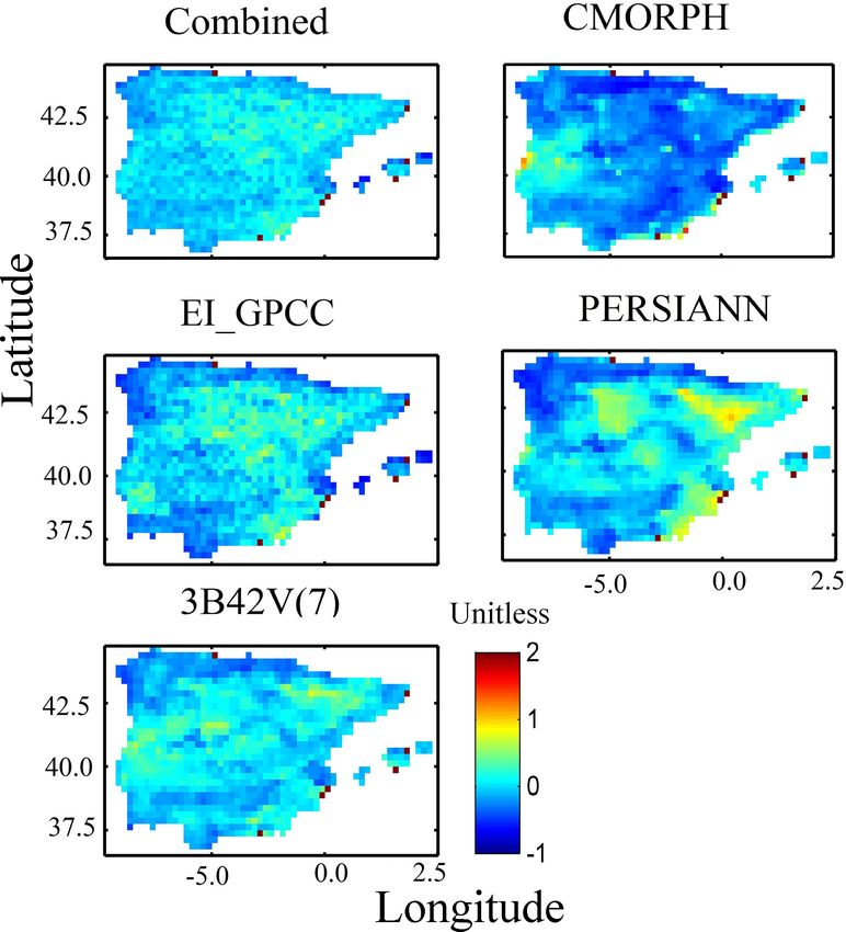
1978                M. A. Ehsan Bhuiyan et al.: Multi-parameter water resource reanalysis uncertainty characterization

3.2    Evaluation metrics                                           the means m and o and standard deviations σm and σo , re-
                                                                    spectively. The CVr includes two components: the ratio of
To examine the magnitude and variability of differences             the means and ratio of the standard deviation. Details on the
among hydrological variables, we used the relative difference       statistical metrics, including name conventions and mathe-
(RD), defined as                                                    matical formulas, are provided in the Appendix.

        ŷi − yi
RD =               ,                                      (1)       3.3   Metrics of uncertainty propagation
            yi
where yi denotes reference variables (SAFRAN-driven sim-            The random error component was based on the normalized
ulations) and ŷi denotes simulated variables (based on the         centered root-mean-square error (NCRMSE). To demon-
other forcing data considered) for each time step i. RD in-         strate how error in precipitation forcing translates to error in
dicates the magnitude and direction of error with positive          the simulated hydrological variables – surface runoff (Qs),
(negative) value indicating overestimation (underestimation).       subsurface runoff (Qsb ), and evapotranspiration (ET) – we
The RD of annual average estimates of the precipitation forc-       used the NCRMSE error metric ratio as follows:
ing and different hydrological variables was calculated using
                                                                                  r
                                                                                    1 Pn
                                                                                            h
                                                                                                        1 Pn
                                                                                                                         i 2
daily datasets at the spatial resolution of 0.25◦ . Moreover, cu-                   n    i=1 ŷi − yi − n   i=1 ŷi − yi
mulative probability of estimated annual average relative dif-      NCRMSE =                  s                               , (5)
                                                                                                    n
ferences among precipitation forcings and the simulated hy-                                      1 P
                                                                                                      (yi − y)2
                                                                                                 n
drological variables were calculated using same spatial reso-                                     i=1
lutions of 0.25◦ .                                                            NCRMSE(simulated variables)
   To collectively assess the performance of various precipi-       αNCRMSE =                             ,                     (6)
                                                                               NCRMSE(precipitation)
tation forcing datasets, models, and simulated hydrological
variables, we used a normalized version of the Taylor di-           where NCRMSE is the normalized centered root-mean-
agram (Taylor, 2001). Specifically, we normalized the val-          square error and αNCRMSE is NCRMSE error metric ratio
ues of the centered root-mean-square error (CRMSE) and              at multiple temporal (3-hourly and daily) and spatial (0.25◦ )
the standard deviation with the standard deviation of the ref-      resolutions. The αNCRMSE metric quantifies the changes in
erence. Therefore, the reference (that is, the target point to      the random error from precipitation to simulated hydrologi-
which the model outputs should be closest) corresponds to           cal variables (Qs , Qsb , and ET) and can thus be used to assess
the point on the graph with the normalized CRMSE equal to           magnification (αNCRMSE > 1) or damping (αNCRMSE < 1).
zero, while both the correlation coefficient and normalized
standard deviation equal 1. The normalized Taylor diagrams          3.4   Analysis of ensemble spread
summarized model results for two different temporal scales
(3-hourly and daily) at the spatial resolution of 0.25◦ .           To assess how variability in the precipitation ensemble trans-
   To evaluate the degree of variation of various precipita-        lates to variability of the various hydrological simulations
tion datasets and simulated hydrological variables, we used         (Qs , Qsb , and ET) for the different modeling systems, we
the coefficient of variation (CV) and coefficient of variation      performed an analysis of ensemble spread (1), formulated
ratio (CVr ). The CV and CVr are determined using all pre-          as
cipitation forcing and variables examined at the 0.25◦ daily
                                                                          Pn
                                                                                (Xmax − Xmin )
resolution. The CV is a measure of variability defined as the       1 = i=1 Pn                  ,                              (7)
                                                                                   i=1 Y
ratio of the standard deviation to the mean. To compare the
degree of variation from one data series to another, we used        in which Xmax and Xmin represent, respectively, the maxi-
the CV where we considered distributions with CV < 1 to             mum and minimum of ensemble values at each time step,
be low variance, while we considered those with CV > 1 to           while Y is the corresponding value of the reference. Here,
be high variance. We defined CVr as the ratio of the CV of          the members of ensemble constitute a sequence for each time
model to the CV of reference. The defined parameters are            step (X1 , X2 . . ..X20 ). The ensemble spread (1) is calculated
expressed as follows:                                               at the monthly scale for the combined product and simu-
       σm                                                           lated hydrologic variables. Note that the combined product
CVm =     ,                                                  (2)    is an ensemble-based precipitation product; for the evalua-
       m
      σo                                                            tions presented in this study, we use the ensemble mean as
CVo = ,                                                      (3)    forcing. For the analysis and propagation of the precipitation
       o
      CVm                                                           ensemble spread to hydrologic simulations, we used 20 en-
CVr =       .                                                (4)    semble members, which are generated stochastically by the
      CVo
                                                                    QRF tree-based regression model (Meinshausen, 2006). 1
The CVm and CVo indicate the coefficient of variation of            provides a measurement of the expected prediction intervals
the model and the coefficient of variation of reference, with       relative to the reference value. The 1 value of 1 indicates

Hydrol. Earth Syst. Sci., 23, 1973–1994, 2019                                     www.hydrol-earth-syst-sci.net/23/1973/2019/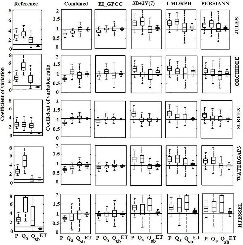
M. A. Ehsan Bhuiyan et al.: Multi-parameter water resource reanalysis uncertainty characterization                              1979

the maximum possible uncertainty of the prediction interval.
To achieve accurate and successful prediction, comparatively
small prediction intervals are expected.

4     Results

4.1    Variability of multiple hydrological model
       simulations

To examine the magnitude and variability of the differences
among both models and forcing datasets, we analyzed the
multi-model simulation results for three hydrological vari-
ables, including surface runoff (Qs ), subsurface runoff (Qsb ),
and evapotranspiration (ET). Throughout this analysis, we
used the SAFRAN-based simulation as the reference for
comparison. Figures 2 to 5 present spatial maps of annual
average values for each model, along with the relative dif-
ferences of annual average estimates of precipitation forcing
and the different hydrological variables for all the precipita-
tion forcing datasets and models. The relative differences in
precipitation forcing (Fig. 2) exhibited considerable spatial
variability for satellite precipitation forcing (relative differ-
ence > 20 %) and relatively lower variability for EI_GPCC           Figure 2. Map of the annual average relative difference (with re-
                                                                    spect to SAFRAN) for the different precipitation forcing datasets.
and the combined product. Examination of SAFRAN-based
annual average values of surface runoff shows that Water-
GAP3 estimates considerably higher surface runoff than the
rest of the models, particularly in the northern and northwest-     ferent model simulations, we can see that WaterGAP3 results
ern part of the study area (Fig. 3). Consequently, subsurface       reveal the lowest relative differences in Qs for almost all the
runoff (Fig. 4) and evapotranspiration (Fig. 5) from Water-         precipitation forcings. In addition, CMORPH-based simula-
GAP3 were lower in that part of the study area. All these           tion underestimated substantially for all the models. Figure 5
results display substantial differences in the spatial pattern      presents the spatial pattern of the results for evapotranspira-
of relative differences, which suggests that simulations are        tion. For the combined product and EI_GPCC, results were
sensitive to both precipitation forcing and model uncertainty.      consistent with low relative difference (< 25 %). On the other
Certain models seem to be more sensitive for given variables.       hand, CMORPH-based simulation showed an overall under-
For example, HTESSEL and ORCHIDEE are the models                    estimation and deviated considerably from the results of the
with the largest relative difference of Qs , and both models ex-    other precipitation products. By examining the spatial pat-
hibited different behaviour relative to the other models when       tern of relative differences (Figs. 2–5), one can recognize
forced by the satellite precipitation. This suggests a distinct     that there is no consistent spatial pattern among the differ-
structural difference in the way precipitation is partitioned       ent model–forcing combinations. There are cases where the
into surface–subsurface runoff between the two groups.              pattern of the differences is dominated by the pattern of pre-
   Looking at the variability of results for combined and           cipitation differences, as, for example, in the case of PER-
reanalysis (EI_GPCC) forcing datasets, no substantial dif-          SIANN, where the maximum number of differences are con-
ferences occurred between reference and simulated sur-              centrated in the central and eastern part of the peninsula.
face runoff (Qs ). However, for the satellite-based simu-           While there are other cases where the pattern is dominated
lations, there were significant deviations. Specifically, the       by the sensitivity of the model (see, for example, results for
CMORPH-based simulation showed significant overestima-              ORCHIDEE and 3B42 for surface runoff).
tion for ORCHIDEE and HTESSEL, but this pattern was re-                We also present a comparison of cumulative probability of
versed for JULES, SURFEX, and WaterGAP3, an outcome                 the relative differences among precipitation forcings (Fig. 6)
that highlights the impact of model structure on precipitation      and the simulated hydrological variables (Fig. 7). The dis-
error propagation.                                                  tribution of relative differences, both in terms of type (de-
   For subsurface runoff, similar spatial patterns (with re-        noted by the shape of the cumulative density function – CDF)
spect to Qs ) were exhibited for the reference and the rest of      and magnitude and differed as a function of precipitation
simulations (Fig. 4), which were also affected substantially        forcing, the model, and the variable considered. The CDF
by precipitation uncertainty. For example, looking at the dif-      of precipitation relative differences shows that CMORPH

www.hydrol-earth-syst-sci.net/23/1973/2019/                                      Hydrol. Earth Syst. Sci., 23, 1973–1994, 2019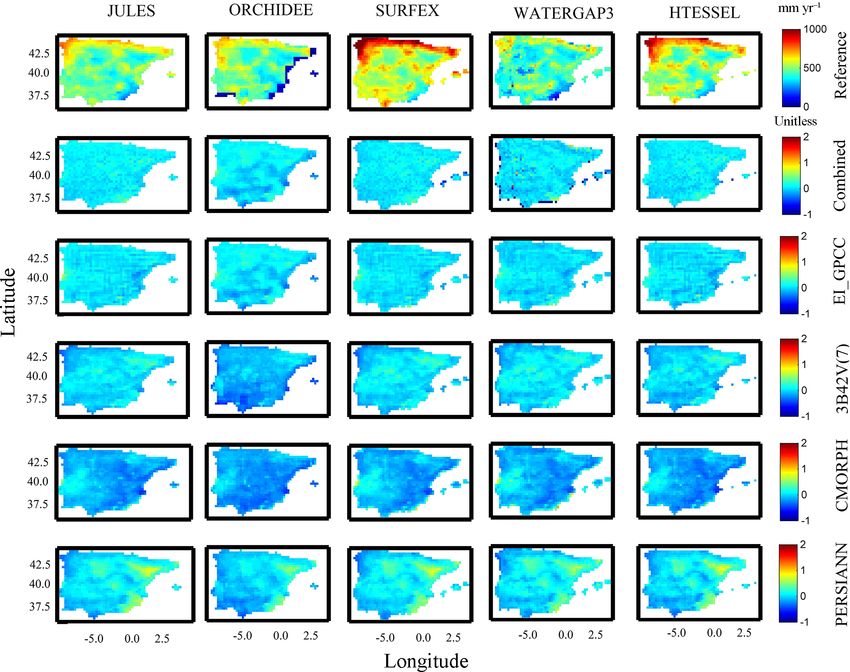
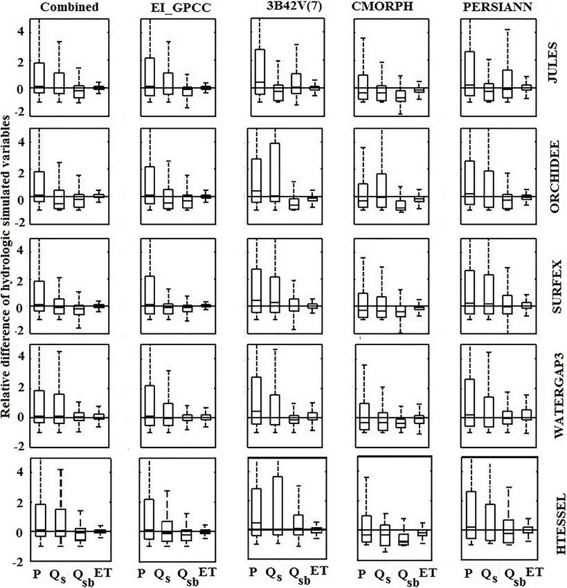
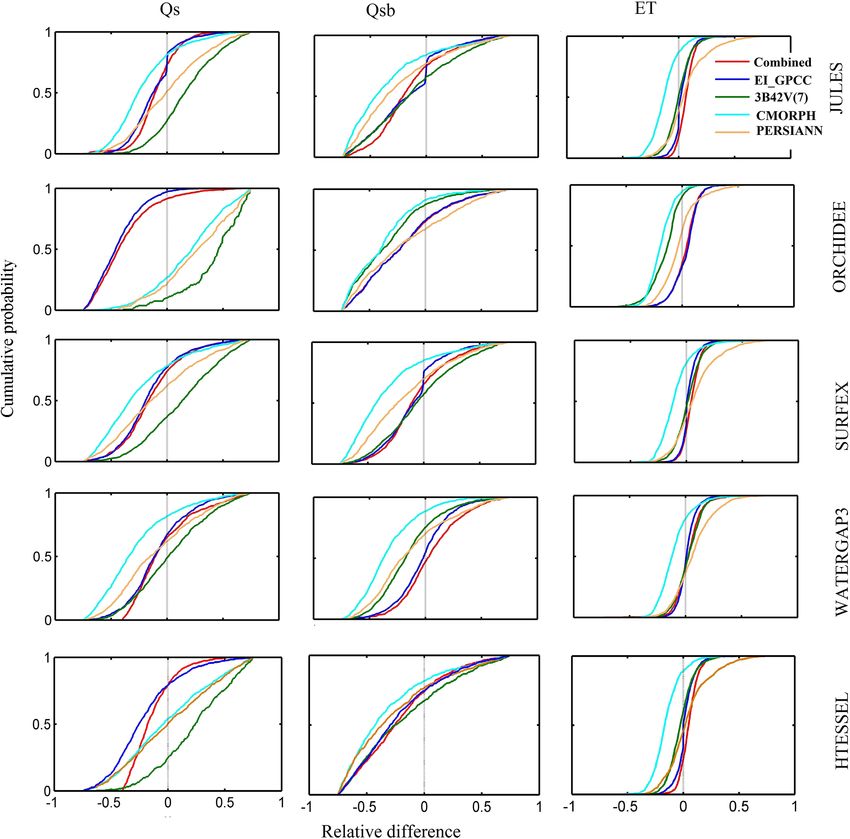
1980               M. A. Ehsan Bhuiyan et al.: Multi-parameter water resource reanalysis uncertainty characterization

Figure 3. Map of SAFRAN-based simulations (Reference) of surface runoff (top row), and relative difference for the various models
(columns) and precipitation forcing (rows 2–5) analyzed.

deviated significantly from the other precipitation products       SURFEX and WaterGAP3 exhibited the lowest variability
(Fig. 6). The surface runoff based on ORCHIDEE and HT-             compared to the other models. Overall, with the exception
ESSEL displayed a clear separation of the CDF for the com-         of few cases (e.g., 3B42V(7) for ORCHIDEE and HTES-
bined product and EI_GPCC and satellite-based precipita-           SEL and CMORPH for ORCHIDEE), uncertainty reduces
tion forcing (Fig. 7). Specifically, it is interesting to note     progressively from precipitation to surface runoff, subsurface
that 3B42V(7) responds very differently to other precipi-          runoff, and finally ET.
tation forcing datasets for ORCHIDEE, highlighting again
the sensitivity of runoff response to precipitation structure      4.2   Performance of multi-model simulations
(space–time variability) and its dependence on the rainfall–
runoff generation mechanism.                                       The normalized Taylor diagrams summarize the results for
   Box plots of the relative difference of different hydrolog-     two different temporal scales. Figure 9 shows the results
ical variables for the various forcing datasets and models at      for the 3-hourly scale only for the two models with output
the daily scale are shown in Fig. 8. Note the inclusion of         available at that resolution (JULES and SURFEX), while
the relative difference of precipitation forcing to allow the      Fig. 10 presents results at the daily scale for all five models.
comparison between relative differences in precipitation with      We aggregated the 3-hourly results from JULES and SUR-
those in the other hydrological variables. For each model, the     FEX to daily to compare them with the nominal daily out-
box plot shows a lower interquartile range (IQR), marking          put of ORCHIDEE, WaterGAP3, and HTESSEL. Results im-
lower variability for Qsb and ET compared to Qs . Results for      proved with the temporal aggregation in reducing random er-
simulations based on the combined product and EI_GPCC              ror for JULES and SURFEX. As shown in Fig. 10, the points
showed less variability than the satellite-based simulations.      for the 3B42V(7) were always the furthest from the refer-

Hydrol. Earth Syst. Sci., 23, 1973–1994, 2019                                    www.hydrol-earth-syst-sci.net/23/1973/2019/
M. A. Ehsan Bhuiyan et al.: Multi-parameter water resource reanalysis uncertainty characterization                            1981

Figure 4. Map of SAFRAN-based simulations (Reference) of subsurface runoff (top row), and relative difference for the various models
(columns) and precipitation forcing (rows 2–5) analyzed.

ence (NCRMSE > 0.75) with the low correlation coefficient           efficient of variation (CV) and the coefficient of variation
(0.4–0.55), except SURFEX, which means that 3B42V(7)                ratio (CVr ) for all the hydrological models. To provide an
was always associated with the worst performance for all            understanding of the impact of precipitation uncertainty in
other models. Simulations based on the combined product             hydrological simulations, we produced box plots of the CV
and EI_GPCC were always consistent, with significantly re-          and CVr for precipitation forcing datasets and individual hy-
duced NCRMSE values in the range of 0.25–0.8 for all the            drological variables for all the models, as shown in Fig. 11.
hydrological models. Results for simulated ET are more con-         A precipitation-forcing-wise comparison indicates that the
sistent among the various precipitation forcing datasets, ex-       combined product and reanalysis underestimated precipita-
hibiting normalized standard deviations in the range of 0.8–        tion variability more than other precipitation forcings, which
1.2. NCRMSE reduced significantly (< 0.35) for each forc-           affected the corresponding variability in Qs for all the mod-
ing dataset; accordingly, the correlation coefficient (CC) also     els except ORCHIDEE. Although there were no significant
raised considerably (> 0.9), showing a very high degree of          differences in terms of variability for combined product and
agreement with reference-based simulations. For surface–            reanalysis-based simulations for the four models (JULES,
subsurface runoff, the SURFEX and WaterGAP3 models per-             SURFEX, WaterGAP3, and HTESSEL), substantial differ-
formed comparatively better than other models by reduc-             ences in variability between precipitation and Qs were ob-
ing NCRMSE values, especially for the combined product              served for ORCHIDEE model. Satellite products overesti-
and EI_GPCC.                                                        mated precipitation variability, leading to overestimation of
   To illustrate the relative variability between precipitation     the variability of surface and subsurface runoff. The vari-
and individual hydrological variables, we calculated the co-        ability of ET was much lower than that of the other vari-

www.hydrol-earth-syst-sci.net/23/1973/2019/                                      Hydrol. Earth Syst. Sci., 23, 1973–1994, 2019
1982               M. A. Ehsan Bhuiyan et al.: Multi-parameter water resource reanalysis uncertainty characterization

Figure 5. Map of SAFRAN-based simulations (Reference) of evapotranspiration (top row), and relative difference for the various models
(columns) and precipitation forcing (rows 2–5) analyzed.

                                                                     ables examined and well captured in all the simulation sce-
                                                                     narios. From the box plots of CV from reference-based simu-
                                                                     lations, the distributions of ET showed low variability (CV <
                                                                     1), while the variability for all the other hydrological vari-
                                                                     ables was high (CV > 1). In terms of CVr , the SURFEX
                                                                     model performed very well by producing medians close to
                                                                     1 (CVr = 1 means ideal consistency) for all the precipitation
                                                                     forcing datasets but CMORPH.

                                                                     4.3   Assessment of precipitation error propagation

                                                                     To investigate the possible amplification, or dampening, of
                                                                     the precipitation error to the hydrologic variables examined,
                                                                     we quantified the NCRMSE error metric ratio (αNCRMSE ),
                                                                     and results are illustrated in Figs. 12 and 13. For all the sce-
                                                                     narios (at 3-hourly and daily scales) and almost all mod-
Figure 6. Cumulative probability for the precipitation forcing       els, αNCRMSE values were less than 1, which highlighted
datasets.                                                            the damping effect on the random error of precipitation in
                                                                     simulated variables. In general, the damping effect increases
                                                                     (i.e., αNCRMSE reduces), moving from surface to subsurface

Hydrol. Earth Syst. Sci., 23, 1973–1994, 2019                                      www.hydrol-earth-syst-sci.net/23/1973/2019/
M. A. Ehsan Bhuiyan et al.: Multi-parameter water resource reanalysis uncertainty characterization 1983
Figure 7. Cumulative probability for the multi-model, multi-forcing simulations for simulated hydrological variables.
runoff and ET and highlighting once again the interaction the relationship between the precipitation ensemble and sim-
between the different runoff-generating mechanisms as well ulated hydrological variables (generated ensemble), we pre-
as coupled water–energy balance processes and precipita- sented an analysis of ensemble spread. Figure 14 depicts
tion uncertainty. Interestingly, the relationship between error density plots between ensemble spread of precipitation and
propagation among the different hydrologic variables var- the simulated hydrological variables (Qs , Qsb , and ET) at
ied greatly between models and precipitation forcing. Val- the monthly scale. A strong correlation between ensemble
ues of αNCRMSE for surface and subsurface runoff are gener- spread of Qs and precipitation is found for almost all mod-
ally close for the SURFEX model but distinctly different for els. For the other variables (ET and Qsb ), ensemble spread
satellite-based results of ORCHIDEE and WaterGAP3. was significantly narrower and rather independent of the en-
semble spread of precipitation, manifested as the horizontal
4.4 Stochastic precipitation ensemble and structure of contours in Fig. 14. The ensemble spread of Qs
corresponding simulated hydrological variable was higher (ORCHIDEE and HTESSEL) or lower (SURFEX
analysis results and WaterGAP3) depending on the model, elucidating again
the impact of the modeling structure on the propagation of
precipitation uncertainty.
The following summarizes the results of our analysis of en-
semble precipitation (20 members), generated stochastically
according to the algorithm used for the combined product,
and their corresponding hydrological simulations. To show
www.hydrol-earth-syst-sci.net/23/1973/2019/ Hydrol. Earth Syst. Sci., 23, 1973–1994, 20191984 M. A. Ehsan Bhuiyan et al.: Multi-parameter water resource reanalysis uncertainty characterization
Figure 8. Relative difference presented for the various products and models at daily scale. In each box, the central mark is the median, and
the edges are the first and third quartiles.
5 Discussion to ET did not deviate significantly among the precipitation
scenarios. This is expected for ET because it is primarily con-
trolled by atmospheric demand, plant and soil hydraulic con-
Precipitation from different satellite–reanalysis datasets ex- straints, and solar radiation (Wallace and McJannet, 2010).
hibits considerable differences in pattern and magnitude, When sufficient energy is available for rainfall to evaporate
which results in significant differences in hydrologic simu- directly without contributing to surface–subsurface runoff,
lations. Results presented in this paper demonstrated clearly simulation of ET is not only affected by precipitation uncer-
that magnitude and dynamics of uncertainty in hydrologic tainty but also by other atmospheric constrains.
simulations depend not only on the uncertainty of the forc- Consequently, results (Figs. 6 to 7) for ET were more con-
ing variable but also on the model and examined hydrologic sistent among the various model and precipitation forcing
variable. scenarios, indicating a smaller degree of uncertainty in ET
For example, surface runoff (Qs ) appears to be highly sen- (relative to Qs and Qsb ). These results suggest that precipita-
sitive to precipitation differences, while ET was not for this tion has a stronger influence on surface runoff, in particular
semi-arid study region (Figs. 3 to 5). Particularly, ET exhib- precipitation intensity, i.e., the same amount of precipitation
ited reduced sensitivity to precipitation forcing, which poten- distributed over 3 h or over 1 d will impact mostly surface
tially suggests that the water volume available for conversion
Hydrol. Earth Syst. Sci., 23, 1973–1994, 2019 www.hydrol-earth-syst-sci.net/23/1973/2019/M. A. Ehsan Bhuiyan et al.: Multi-parameter water resource reanalysis uncertainty characterization 1985
Figure 10. Normalized Taylor diagrams for daily simulated hydro-
logical variables with SAFRAN and the satellite–reanalysis precip-
Figure 9. Normalized Taylor diagrams for 3-hourly precipitation itation products used.
and simulated hydrological variables based on SAFRAN and the
satellite–reanalysis precipitation products used.
differences of their corresponding surface runoff generation
modules.
Evaluation of the performance of the various simulations,
runoff, and this is associated with the model representation relative to SAFRAN, emphasized the issues due to low cor-
of this fast process. Similarly, if we look at the distribution relation and increased random error from satellite products.
of precipitation relative difference, CMORPH tends to de- On the other hand, the reanalysis (EI_GPCC) and combined
crease in magnitude compared to other precipitation prod- product resulted in reduction of random error, suggesting that
ucts. Therefore, for subsurface runoff, CMORPH-based sim- relying on gauge-adjusted reanalysis or blended (satellite–
ulations displayed a gross underestimation compared to other reanalysis) products offers improvement relative to satellite
precipitation forcing. products alone.
Precipitation-to-surface-runoff sensitivity is strongly con- Certain dynamics resolved from this analysis were gener-
trolled by the corresponding runoff generation scheme in ally consistent among different models, such as the fact that
each model. For example, in the case of HTESSEL and OR- uncertainty reduced systematically from precipitation to sur-
CHIDEE, precipitation intensity has a great effect on the gen- face runoff to subsurface runoff and eventually to ET sim-
eration of surface runoff. The satellite precipitation datasets ulations. This is also in accordance with our expectations,
have higher precipitation intensities (Fig. 6) when compared given that soil moisture (storage) integrates the precipitation
to the remaining datasets, which explains the different be- variability in time. Surface runoff exhibits high correlation to
haviour of these two models. However, in the case of JULES, precipitation, while uncertainty in subsurface runoff is mod-
the infiltration excess mechanism is rarely invoked when the ulated by storage capacity of the soils. In addition ET is af-
drivers are provided at a 3-hourly time step, as the maximum fected only if water availability deviates significantly from
infiltration rate is not reached. Therefore, the significance the water demand in terms of potential evapotranspiration.
of differences that HTESSEL and ORCHIDEE show with Our findings related to the surface runoff uncertainty (due
more intense rainfall are not shown by JULES due to distinct to model structure and precipitation) suggest that the use of
www.hydrol-earth-syst-sci.net/23/1973/2019/ Hydrol. Earth Syst. Sci., 23, 1973–1994, 20191986 M. A. Ehsan Bhuiyan et al.: Multi-parameter water resource reanalysis uncertainty characterization
Figure 11. Relationship between coefficient of variation and coefficient of variation ratio of simulated hydrological variables and precipita-
tion.
surface runoff (e.g., flash floods diagnostics) should be care- system. Hydrological simulations based on reanalysis and
fully considered in each application in view of each model combined product forcing datasets performed better over-
formulation. all than satellite precipitation-driven simulations. Moreover,
simulation results using CMORPH as forcing exhibit over-
all overestimation for ORCHIDEE and HTESSEL, which
6 Conclusions is totally the opposite to the results from the other models
(JULES, SURFEX, and WaterGAP3). These types of dif-
This study investigated the propagation of precipitation un- ferences highlight the complexity of the interaction between
certainty in hydrological simulations and its interaction precipitation characteristics and different modeling schemes
with hydrologic modeling, which was based on satellite– and should be used as a “reference for caution” when gener-
reanalysis precipitation forcing of a number of global hydro- alizing findings produced from single model simulations.
logical and land surface models for the Iberian Peninsula. Modeling uncertainty appeared to be much less important
The following are the major conclusions from this study. for evapotranspiration than for surface and subsurface runoff.
Simulation of surface runoff was shown to be highly sen- The sensitivity of hydrological simulations to different pre-
sitive to precipitation forcing, but the direction (that is, over- cipitation forcing datasets was shown to depend on the hy-
estimation or underestimation) and the magnitude of rela- drological variable use and model parameterization scheme.
tive differences indicated strong dependence on the modeling
Hydrol. Earth Syst. Sci., 23, 1973–1994, 2019 www.hydrol-earth-syst-sci.net/23/1973/2019/M. A. Ehsan Bhuiyan et al.: Multi-parameter water resource reanalysis uncertainty characterization 1987
Figure 12. NCRMSE error metric ratios presented for the various
products and models at 3-hourly scale.
Figure 14. Density contour plot of the relationship between ensem-
ble spread of simulated hydrological variables and precipitation at
monthly scale. Color scale shows the frequency of occurrence. The
black line is the 1 : 1 line.
modeling approach. This study assessed the multi-model
performances regarding three different hydrologic variables
(surface–subsurface runoff and evapotranspiration). Apart
from precipitation forcing, other atmospheric forcing vari-
ables required for the hydrologic simulations are also essen-
tial in investigating the significance of hydrological model
uncertainty. In addition, the only calibrated model in this
study, WaterGAP3, performs better in specific locations (e.g.,
hilly) for all the hydrologic variables than other models.
Therefore, investigation should be performed in calibrating
and regionalizing models for different parameters. Neverthe-
Figure 13. NCRMSE error metric ratios presented for the various less, a clear outcome of the current work is that uncertainty in
products and models at daily scale. hydrologic predictions is significant and should be assessed
and quantified in order to foster the effective use of the out-
puts of global land surface models and hydrologic models.
Finally, based on our evaluation of the performance of the Considering ensemble representation (e.g., multi-model and
different hydrological models and five precipitation prod- multi-forcing) of hydrologic variables provides an appropri-
ucts – CMORPH, PERSIANN, 3B42V(7), reanalysis, and ate path to address this issue.
the combined product – we could not identify a single model Advancing our understanding of precipitation uncertainty,
that consistently outperformed others, i.e., certain models ap- model uncertainty, and their interaction will potentially also
peared to be more successful in the simulation of certain vari- aid in the investigation of the impacts of climate change (and
ables. associated uncertainty) on hydrological cycle components
This study suggests that important benefits may accrue and water resource systems. Finally, this research provides
from exploring different model structures as part of the a fine platform for discussing advances in the applications of
www.hydrol-earth-syst-sci.net/23/1973/2019/ Hydrol. Earth Syst. Sci., 23, 1973–1994, 20191988 M. A. Ehsan Bhuiyan et al.: Multi-parameter water resource reanalysis uncertainty characterization different precipitation algorithms, hydrology, and water re- source reanalysis. Data availability. The datasets are available online for SAFRAN (http://mistrals.sedoo.fr/Data-Download-IPSL/ ?datsId=1388&search=0&project_name=HyMeX, last access: 31 March 2019), CMORPH (ftp://ftp.cpc.ncep.noaa.gov/precip/ CMORPH_V1.0/RAW/0.25deg-3HLY/, last access: 31 March 2019), PERSIANN (http://fire.eng.uci.edu/PERSIANN/data/ 3hrly_adj_cact_tars/, last access: 31 March 2019), 3B42V(7) (https://mirador.gsfc.nasa.gov, last access: 31 March 2019), the at- mospheric reanalysis dataset (https://wci.earth2observe.eu/portal/, last access: 31 March 2019), and the combined product (https://sites.google.com/uconn.edu/ehsanbhuiyan/research, last access: 31 March 2019). Hydrol. Earth Syst. Sci., 23, 1973–1994, 2019 www.hydrol-earth-syst-sci.net/23/1973/2019/
M. A. Ehsan Bhuiyan et al.: Multi-parameter water resource reanalysis uncertainty characterization             1989

Appendix A

The statistical metric, the coefficient of variation ratio (CVr )
used in the model evaluation analysis, was computed using
the following parameters:
        N
     1 X
o=         oi ,                                            (A1)
     N i=1
        N
     1 X
m=         mi ,                                            (A2)
     N i=1
     v
           N
     u
     u1 X
σo = t        (oi − o)2 ,                                  (A3)
       N i=1
     v
           N
     u
     u1 X
σm = t         (mi − m)2 .                                 (A4)
        N i=1

   Here, oi and mi (i = 1, . . ., N ) are the observed and mod-
eled time series, respectively, of the product for times i, with
the means o and m and standard deviations σo and σm , re-
spectively; N is the total number of data points used in the
calculations.

www.hydrol-earth-syst-sci.net/23/1973/2019/                            Hydrol. Earth Syst. Sci., 23, 1973–1994, 2019
1990 M. A. Ehsan Bhuiyan et al.: Multi-parameter water resource reanalysis uncertainty characterization
Table A1. Information on precipitation products used.
Original spatiotemporal
Model resolution References
SAFRAN 5 km, 1 h Quintana-Segui et al. (2016)
Combined 0.25◦ , 3 h Bhuiyan et al. (2018)
EI_GPCC 0.25◦ , 3 h https://wci.earth2observe.eu/portal/
(last access: 31 March 2019)
3B42V (7) 0.25◦ , 3 h Huffman et al. (2010)
CMORPH 0.25◦ , 3 h Joyce et al. (2004)
PERSIANN 0.25◦ , 3 h Sorooshian et al. (2000)
Table A2. Details of the modeling systems.
Evapotrans- Soil Ground Reservoirs/ Routing Model
Model Interception piration layers water Runoff Lakes scheme time step
JULES Single reservoir, Penman– 4 No Saturation and No No 1h
potential Monteith infiltration
evapotranspiration excess
ORCHIDEE Single reservoir Bulk ETP 11 Yes Green–Ampt No Linear cascade 900 s energy
structural (Barella- infiltration of reservoirs balance, 3 h
resistance to Ortiz et (sub-grid) routing
evapotranspiration al., 2013)
SURFEX Single reservoir, Penman– 14 Yes Saturation and No TRIP with 900 s for
potential Monteith infiltration stream and ISBA,
evapotranspiration excess deep-water 3600 s for
reservoir at 0.5◦ TRIP
WATERGAP3 Single reservoir Priestley– 1 Yes Beta function Yes Manning– 1d
Taylor Strickler
HTESSEL Single reservoir, Penman– 4 No Saturation No CaMa-Flood 1h
potential Monteith excess
evapotranspiration
Hydrol. Earth Syst. Sci., 23, 1973–1994, 2019 www.hydrol-earth-syst-sci.net/23/1973/2019/You can also read