Unsaturated zone model complexity for the assimilation of evapotranspiration rates in groundwater modelling
←
→
Page content transcription
If your browser does not render page correctly, please read the page content below
Hydrol. Earth Syst. Sci., 25, 2261–2277, 2021
https://doi.org/10.5194/hess-25-2261-2021
© Author(s) 2021. This work is distributed under
the Creative Commons Attribution 4.0 License.

Unsaturated zone model complexity for the assimilation of
evapotranspiration rates in groundwater modelling
Simone Gelsinari1,2,a , Valentijn R. N. Pauwels1 , Edoardo Daly1 , Jos van Dam3 , Remko Uijlenhoet4,5 ,
Nicholas Fewster-Young6 , and Rebecca Doble2
1 Department  of Civil Engineering, Monash University, Clayton, VIC, Australia
2 CSIRO   Land and Water, Waite Campus, Glen Osmond, SA, Australia
3 Soil physics and Land Management, Wageningen University & Research, Wageningen, the Netherlands
4 Hydrology and Quantitative Water Management Group, Wageningen University & Research, Wageningen, the Netherlands
5 Department of Water Management, Delft University of Technology, Delft, the Netherlands
6 UniSA STEM, University of South Australia, Adelaide, SA, Australia
a Now at: Department of Civil, Environmental and Mining Engineering, University of Western Australia,

Perth, WA, Australia

Correspondence: Simone Gelsinari (simone.gelsinari@monash.edu) and Valentijn Pauwels
(valentijn.pauwels@monash.edu)

Received: 25 May 2020 – Discussion started: 6 July 2020
Revised: 12 March 2021 – Accepted: 12 March 2021 – Published: 27 April 2021

Abstract. The biophysical processes occurring in the unsat-       found that, once properly calibrated to reproduce the actual
urated zone have a direct impact on the water table dynam-        evapotranspiration–water table dynamics, a simple concep-
ics. Representing these processes through the application of      tual model may be sufficient for this purpose; thus using one
unsaturated zone models of different complexity has an im-        configuration over the other should be motivated by the spe-
pact on the estimates of the volumes of water flowing be-         cific purpose of the simulation and the information available.
tween the unsaturated zone and the aquifer. These fluxes,
known as net recharge, are often used as the shared variable
that couples unsaturated to groundwater models. However, as
                                                                  1   Introduction
recharge estimates are always affected by a degree of uncer-
tainty, model–data fusion methods, such as data assimilation,     Actual evapotranspiration (AET) and groundwater recharge
can be used to inform these coupled models and reduce un-         to the water table (WT) are two interrelated components of
certainty. This study assesses the effect of unsaturated zone     the water cycle. This is because AET is a function of the soil
models complexity (conceptual versus physically based) to         water content within the root zone, as the root water uptake
update groundwater model outputs, through the assimilation        is distributed along the entire root system (Grinevskii, 2011;
of actual evapotranspiration rates, for a water-limited site in   Neumann and Cardon, 2012). Improving AET estimates, by
South Australia. Actual evapotranspiration rates are assimi-      means of a detailed modelling of the soil water transport,
lated because they have been shown to be related to the wa-       can enhance the simulation of net recharge (i.e. recharge to
ter table dynamics and thus form the link between remote          the WT minus transpiration from WT) and, in turn, WT dy-
sensing data and the deeper parts of the soil profile. Re-        namics. This is particularly important when the WT is within
sults have been quantified using standard metrics, such as the    the reach of the roots, as is common in Australian semi-arid
root mean square error and Pearson correlation coefficient,       catchments (Banks et al., 2011) because the root water up-
and reinforced by calculating the continuous ranked prob-         take from groundwater and the capillary fringe can largely
ability score, which is specifically designed to determine a      contribute to AET (Mensforth et al., 1994; Orellana et al.,
more representative error in stochastic models. It has been       2012).

Published by Copernicus Publications on behalf of the European Geosciences Union.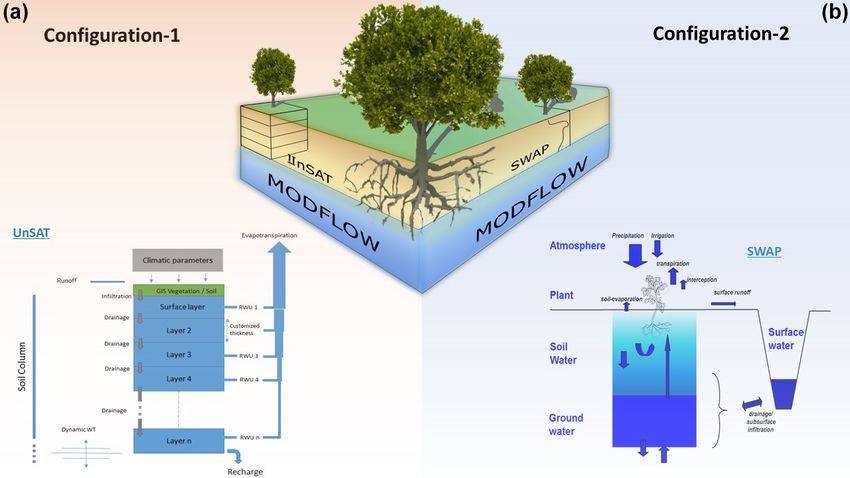
2262             S. Gelsinari et al.: Unsaturated zone model complexity for the assimilation of evapotranspiration rates

   AET is often simulated through a variety of numer-                One way to make use of the remote sensing observations
ical models that reproduce the soil water–vegetation in-          is through data assimilation, which combines model results
teraction with different level of details. Advanced inte-         with independent observations to reduce model uncertainty.
grated surface water–groundwater models (e.g. Hydrogeo-           In the field of hydrology, there is a plethora of studies on
sphere, Therrien et al., 2006; CATHY, Camporese et al.,           the assimilation of diverse observations such as soil mois-
2010; PARFLOW, Jones and Woodward, 2001) or cou-                  ture (SM), leaf area index, and streamflow and groundwa-
pled saturated–unsaturated zone models (Facchi et al., 2004;      ter levels (Liu et al., 2012; Li et al., 2016). Satellite remote
Simunek et al., 2009; Zhu et al., 2012; Van Walsum and Veld-      sensing data have been proven to be a valid alternative when
huizen, 2011; Grimaldi et al., 2015) are able to account for      field-based observations cannot provide sufficiently accurate
the direct groundwater–vegetation interaction. In general, the    measurements. Remotely sensed SM values are a function
representation of the unsaturated zone is obtained from sim-      of the water content of the upper few centimetres of the soil
ple conceptual water balance models or detailed physically        (Pipunic et al., 2014). Consequently, models using remotely
based models.                                                     sensed SM assimilation extrapolate the update for the upper
   Conceptual unsaturated zone models (UZMs) simplify the         soil layer to the entire modelled soil column through the co-
processes occurring in the unsaturated zone and are widely        variance between the upper and lower layer modelled SM
used for spatially distributed hydrological simulations (Teul-    values. On the other hand, remotely sensed AET rates are a
ing and Troch, 2005). An example is Batelaan and De Smedt         function of the modelled water content of the soil column up
(2007), who successfully applied a coupled surface water–         to the rooting depth. In consideration of this, the assimilation
groundwater balance model at the regional scale, focusing         of remotely sensed AET has the potential of directly updat-
on the assessment of net recharge rates. Conceptual water         ing the water content of the entire modelled soil column. In
balance models have been found to be flexible as they usu-        recent years, the assimilation of satellite-based AET obser-
ally require shorter run times and fewer parameters and are       vations has been recognised to be beneficial for the reduction
suitable when stochastic simulations based on Monte Carlo         of the uncertainty of several hydrogeological products (e.g.
techniques are applied (Kim and Stricker, 1996; Fatichi et al.,   recharge and depth to WT), especially for data-scarce areas
2016). However, for more detailed simulations, such as in         (Entekhabi and Moghaddam, 2007; Doble et al., 2017; Gelsi-
ecohydrology or agricultural modelling, simple UZMs may           nari et al., 2020).
fail to accurately simulate important processes such as wa-          All satellite observations present a trade-off between ac-
ter stress or root growth (Krysanova and Arnold, 2008); thus      curacy, time frequency, and spatial coverage. In addition, no
physically based models are preferred. Commonly, physi-           satellite retrievals are free from errors, as discussed in Long
cally based models solve the Richards equation for water          et al. (2014), who analysed and compared the uncertainty
flow in porous media, relying on relationships between soil       in the AET estimates from different sources, including the
volumetric water content, hydraulic conductivity, and soil        Moderate-Resolution Imaging Spectroradiometer (MODIS).
water pressure head (van Dam et al., 2008; Scheerlinck et al.,    They concluded that AET derived from land surface mod-
2009). Physically based models thus have the ability to ac-       els had a lower uncertainty than the MODIS-based AET (5
count for specific effects that affect the calculation of AET,    vs. 12.5 mm per month, respectively) and suggested a hybrid
such as capillary rise, thereby impacting net recharge esti-      approach for taking advantage of the integration of land sur-
mates. The latter is particularly important when UZMs are         face models and remotely sensed products. Droogers et al.
coupled to saturated models as net recharge acts as the link      (2010) applied an inverse modelling approach (i.e. forward–
between both models (Doble et al., 2017).                         backwards optimisation) using a physically based UZM and
   Given the spatial variability and number of parameters         found that improvements were obtained when the frequency
(e.g. the water retention curve and detailed vegetation char-     of the AET observations was finer than a 15 d interval. It
acteristics) required by physically based models, their appli-    appears that, for the purpose of proficiently using AET re-
cation, particularly in data-scarce areas, can be challenging     trievals, the assimilation framework should allow for fre-
(Simmons and Meyer, 2000). Conversely, conceptual models          quent updates (< 15 d interval) and account for observation
may require fewer input data, but, their recharge estimates       errors. This was also synthetically shown by Gelsinari et al.
may be less reliable. This occurs because they are affected       (2020), who improved the model outputs, using the ensem-
by both structural uncertainty, induced by the simplification     ble Kalman filter (EnKF) for the sequential assimilation of
of the model (Renard et al., 2010), and the epistemic and         the averaged 8 d AET into a conceptual UZM coupled to
aleatory uncertainty of the forcing inputs (Khatami et al.,       MODFLOW (Harbaugh, 2005). The assimilation of satellite
2019). Accurate model parameters and meteorological in-           AET observations has been shown to be a feasible way to
puts are far from always available, especially at large spatial   constrain hydrologic models; however, this has yet to be val-
scales. Therefore, the use of remote sensing data can provide     idated against experimental data. Furthermore, it is known
vital information for these models (Entekhabi and Moghad-         that UZMs of different complexity can yield different AET
dam, 2007; Carroll et al., 2015; Lu et al., 2020).                estimates, producing distinct recharge values and, in turn, a
                                                                  diverse dynamics of the WT.

Hydrol. Earth Syst. Sci., 25, 2261–2277, 2021                                      https://doi.org/10.5194/hess-25-2261-2021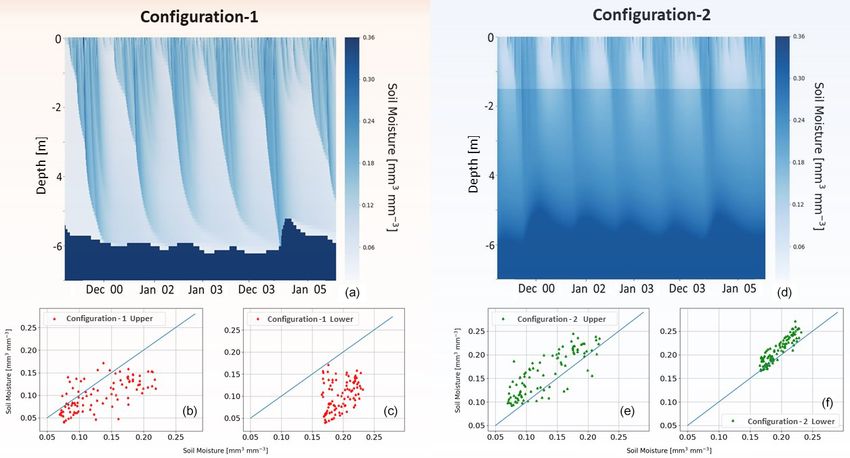
S. Gelsinari et al.: Unsaturated zone model complexity for the assimilation of evapotranspiration rates 2263
This study aims to perform the validation of the AET as- tained from MODIS (Swaffer et al., 2020). The observations
similation framework proposed in Gelsinari et al. (2020) and are available every 8 d, with a spatial resolution of 250 by
to assess the use of a conceptual and a physically based UZM 250 m.
within a data assimilation framework to improve WT esti-
mates. The quantities of interest are the temporal WT fluc- 2.2 Model description
tuation dynamics and the modelled actual AET. A concep-
tual and a physically based UZM are coupled to MODFLOW The tests presented in this study used two different config-
and applied to a water-limited study site in the south-east of urations of coupled groundwater–unsaturated zone models,
South Australia. Remotely sensed AET observations are as- which are depicted in Fig. 2. The following sections describe
similated into both of these coupled models, and assessments the models as well as the coupling framework.
of the improvements in the results of the model are made.
Based on this assessment, a number of recommendations re- 2.2.1 UnSAT – UZM
garding the required UZM complexity to obtain a positive
The UnSAT (Unsaturated zone and SATellite) UZM is a one-
impact on the quantities of interest are made.
dimensional soil water balance model. The unsaturated zone
is divided into layers, and the water balance of each layer is
solved at every time step. Water flows downward from the top
2 Methods layer to the last, and the latter delivers recharge (Fig. 2). The
model uses climate forcing data (i.e. precipitation [mm h−1 ]
2.1 Study area and data
and PET [mm h−1 ]) on a raster-distributed basis as inputs and
returns values of AET [mm h−1 ], runoff [mm h−1 ], recharge
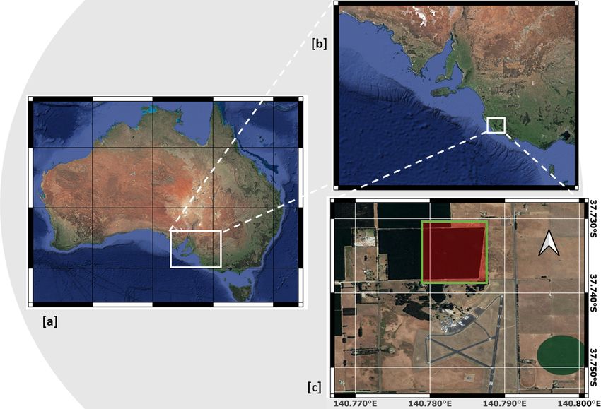
The study area is situated in the south-eastern part of South
[mm h−1 ], and soil water content (θ [mm3 mm−3 ]). The soil
Australia, north of the city of Mount Gambier (Fig. 1a and
is parameterised using the porosity (θs ), a critical soil wa-
b). This region has a Mediterranean climate with cool, wet
ter content to define water stress (θ∗ [mm3 mm−3 ]), residual
winters and warm, dry summers. The climatic forcing inputs
soil water content (θr [mm3 mm−3 ]) (as in Laio et al., 2001),
are rainfall and potential evapotranspiration (PET) obtained
hydraulic conductivity (Ks [mm3 mm−3 ]), and an empirical
from the Bureau of Meteorology (BOM – station no. 26021).
value for drainage (b [–]); the root system is defined using
The historical data for this station report an average annual
root depth (lr [mm]) and a root density distribution parame-
rainfall and PET of approximately 710 and 980 mm yr−1 , re-
ter (Vr [–]) (Vrugt et al., 2001a).
spectively, calculated over the period 1942–2017. The Mor-
The size of the layers (1z [mm]) remains constant, while
ton equation (Donohue et al., 2010) and the Budyko curve
their number changes according to the depth to WT, which is
(Donohue et al., 2007) classify the area as dominated by
provided by the groundwater model. Along the soil profile,
evapotranspiration or water-limited (Jackson et al., 2009;
the model accounts for water extraction due to root water
Benyon et al., 2006).
uptake. For each layer, the water balance equation is solved
The study site is a Pinus Radiata plantation next to Mount
using an explicit finite difference approximation, solved with
Gambier Airport (Fig. 1c). The trees were originally planted
an hourly time step (1t). The water balance of the layer at
in July 1996 with a density of 1225 trees per hectare. The
the soil surface is calculated as
survey performed by Benyon et al. (2006) classified the soil
as duplex. This type of soil presents a contrast between the P t − AETt1 − Qt − D1t
upper part, which features sandy loam characteristics with θ1t+1 = θ1t + · 1t , (1)
1z1
high hydraulic conductivity, and the lower part, classified as
clay, with a finer texture and lower hydraulic conductivity. where P is precipitation, Q is runoff and D is percolation.
The average WT depth, from the observations at one bore, is In Eq. (1), the subscripts 1 refer to the soil layer at the sur-
reported at approximately 6 m below the surface. SM obser- face, and the superscripts refer to the time step. The percola-
vations were taken with a neutron probe, about every 4 weeks tion D1t , which proceeds to the lower layer, is defined by the
from August 2000 to January 2005, up to a depth of 3 m at Clapp–Hornberger (Clapp and Hornberger, 1978) modifica-
an interval of 30 cm. In this region more than 90 % of the tion of the Brooks–Corey model.
available groundwater is in shallow aquifers, and these plan- AET is calculated as
tations have been shown to have direct access to groundwater
(Benyon and Doody, 2004). AET = PET · β(z) · α(θ ), (2)
AET data are derived from the remotely sensed
CSIRO MODIS-reflectance-based scaling evapotranspira- where β(z) is the root distribution function as in Vrugt et al.
tion (CMRSET) algorithm (Guerschman et al., 2009). These (2001b), and α is a water stress reduction function (Laio
values are obtained by rescaling the PET rates calculated et al., 2001; Feddes et al., 1976).
with the Penman–Monteith algorithm using the enhanced For the layers below the first, including the last layer,
vegetation index and global vegetation moisture index ob- which delivers recharge to the groundwater model, the wa-
https://doi.org/10.5194/hess-25-2261-2021 Hydrol. Earth Syst. Sci., 25, 2261–2277, 2021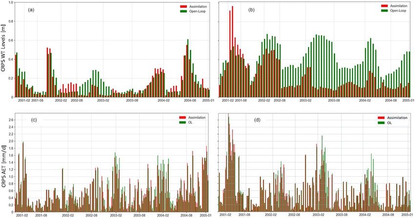
2264               S. Gelsinari et al.: Unsaturated zone model complexity for the assimilation of evapotranspiration rates

Figure 1. Localisation of the study area within Australia (a), the south-east of South Australia (b), and a detail of the forest plantation (c).
The red square indicates the CMRSET tile. © Google Maps

Figure 2. Coupled models’ representation. (a) UnSAT conceptualisation coupled to MODFLOW. (b) SWAP conceptualisation coupled to
MODFLOW.

ter balance equation is                                                   2.2.2    SWAP UZM
                 t
                Dn−1 − (AETtn + Dnt )
θnt+1 = θnt +                            · 1t .                  (3)      The Soil Water Atmosphere Plant (SWAP v. 4.0) model, de-
                         1zn                                              veloped by Alterra, is one of the most used physically based
For a more detailed description of the UnSAT model, see                   UZMs (van Dam et al., 2008; Kroes et al., 2017). This agro-
Gelsinari et al. (2020).                                                  hydrological model is able to simulate the water, heat, and
                                                                          solute flow in heterogeneous, variably saturated soils. Water
                                                                          flow is simulated using the Richards equation. In addition,

Hydrol. Earth Syst. Sci., 25, 2261–2277, 2021                                                https://doi.org/10.5194/hess-25-2261-2021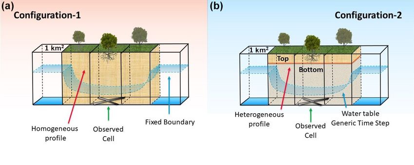
S. Gelsinari et al.: Unsaturated zone model complexity for the assimilation of evapotranspiration rates                   2265

it has the potential of accounting for a detailed soil water–    of layers in which the unsaturated zone is discretised. This
vegetation interaction as it specifically simulates the dynam-   dynamic scheme, defined in Zeng et al. (2019) as the non-
ics of the crop growth cycle.                                    iterative feedback coupling method, is considered a valuable
   In SWAP, the Richards equation is solved for the pres-        trade-off between the computational cost of fully coupled or
sure head using finite differences. The soil hydraulic reten-    iterative schemes and numerical accuracy.
tion functions are based on the analytical formulations pro-        For Configuration-2 (Fig. 2b), the unsaturated zone is sim-
posed by van Genuchten (1980). The model requires the            ulated through the SWAP model, with the pressure head
van Genuchten soil parameters and a number of vegetation-        along the soil column as the state variable. The model has
specific parameters (Feddes et al., 1976). In this study, the    been coupled to MODFLOW through the recharge, similar
parameters accounting for the drought stress, which are the      to the coupling methodology reported by Xu et al. (2012).
pressure head value below which water uptake reduction           This type of coupling requires caution in the definition of the
starts (i.e. −3000 mm) and the pressure head value triggering    Sy parameter, which becomes part of the calibration and is
no further water extraction (i.e. −30 000 mm), are a result of   discussed in the next section.
the calibration. For this experiment, the standard forest root
density distribution is applied.                                 2.3   Model domain and calibration

2.2.3   Groundwater model                                        The model configurations were applied to a domain of 1 × 5
                                                                 cells of 1 km2 each and a single vertical unconfined layer
The groundwater model chosen for the study is MODFLOW            (Fig. 3). The domain discretisation was chosen as a result of
2005 (Harbaugh, 2005). This modular flexible model has           a sensitivity analysis conducted on a range of model domains
packages dedicated to the calculation of evapotranspiration      varying from fine (1 × 20 cells) to coarse (1 × 5 cells). The
and the application of recharge to the groundwater. In this      boundary cells were set to a constant head obtained via cal-
study, the evapotranspiration package of MODFLOW (EVT)           ibration (i.e. 3.5 m below the surface). The location chosen
was replaced with the UZMs (UnSAT and SWAP), and the             allows the model configuration to remain simple and to de-
recharge (RCH) package was used to apply the UZMs’ cal-          fine constant head boundary conditions. This is due to the site
culated net recharge to the cell-specific head.                  being in the centre of a forestry block, more than 2 km from
   FloPy (Bakker et al., 2016), a library that allows MOD-       any groundwater extraction. For this region, where WT is 6 m
FLOW to run in a Python environment, was used to generate        deep or shallower, it has been shown that forestry transpira-
the saturated model and to specify parameters. The model         tion from groundwater is around 2 orders of magnitude (i.e.
runs at an 8 d time step, which is considered adequate for       435 ML yr−1 for a 1 km by 1 km fully forested cell) larger
WT dynamics. This choice was motivated by matching the           than the maximum groundwater extraction rate from a single
temporal resolution of the CMRSET data.                          bore (Benyon et al., 2006). To further reinforce the selection
                                                                 of constant head boundary conditions, an analysis of the WT
2.2.4   Coupling                                                 fluctuations was conducted on bores in the proximity of the
                                                                 study area but outside of the forest. The analysis showed that,
UZMs require a shorter time step than MODFLOW as the             for a WT level of 4.4 m below the surface, the standard de-
water content varies at a higher frequency than the depth to     viation was low (i.e. 0.12 m). This supports the assumption
the WT in the groundwater model (Xu et al., 2012). Variation     that, if higher WT table fluctuations are observed (such as
of the WT at regional scales usually can only be observed at     the investigated location), these are dependent on the local
temporal scales in the order of months or years. Thus, apply-    net recharge.
ing a larger time step for the saturated zone model is a valu-      UnSAT can account for the decrease of Ks along the
able option to reduce the computational time (Facchi et al.,     soil column, whereas SWAP is capable of explicitly mod-
2004). At large spatial scales, dimensional simplification to    elling the heterogeneity of the soil column, as described in
1D unsaturated zone flow simulations has been shown to be        Sect. 2.1. Thus, for Configuration-1, soil parameters are ho-
sound because the direction of the unsaturated zone flow is      mogeneous along the soil column length (i.e. 10 m or 100
predominantly vertical (Zhu et al., 2011).                       layers of 10 cm), while in Configuration-2, the first (upper)
   Configuration-1 (Fig. 2a) features the UnSAT model cou-       1.5 m of soil is classified as sandy loam soil, and the second
pled to MODFLOW. This configuration specifically accounts        (lower) is a loam clay soil spanning the rest of the simulated
for plant transpiration from the WT by calculating the bal-      soil column (i.e. 8.5 m).
ance between recharge entering the WT (positive) and tran-          In order for the system to be observable, the link be-
spiration (negative). UnSAT runs at an hourly time step,         tween WT levels and AET has to be accurately reproduced.
while MODFLOW runs with an 8 d time step, matching the           It should be noted that this link has been described in the
MODIS time step. Once MODFLOW has performed the cal-             literature (Shah et al., 2007; Xie et al., 2018; Zhang et al.,
culation of the WT levels, these are fed back on a raster ba-    2020). To account for this interdependence, a multi-objective
sis to UnSAT, which uses them to recalculate the number          function (MOF), which combines WT depths and AET val-

https://doi.org/10.5194/hess-25-2261-2021                                     Hydrol. Earth Syst. Sci., 25, 2261–2277, 2021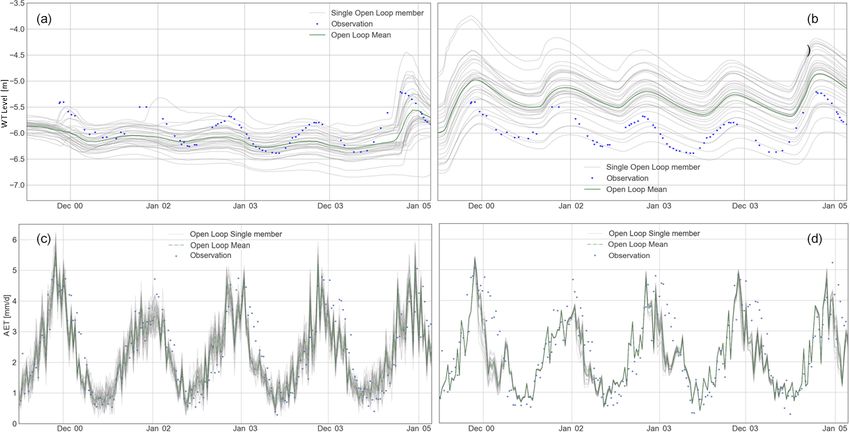
2266              S. Gelsinari et al.: Unsaturated zone model complexity for the assimilation of evapotranspiration rates

Figure 3. Schematic of the model domain. (a) Configuration-1 models the unsaturated zone as a homogeneous profile with UnSAT. (b)
Configuration-2 models the soil heterogeneity by accounting for the change in soil properties with SWAP. The representation of WT levels
refers to the generic simulation time and is conceptually showing the depression caused by the root water extraction.

ues, was introduced. Then, SM observations were used for              Therefore, the interaction between AET and model states oc-
refinement and to set boundaries to the soil parameters. The          curs in the UZM, of which AET is a model result. Following
algorithm particle swarm optimisation (PSO) (Kennedy and              Gelsinari et al. (2020), AET data from the CMRSET are as-
Eberhart, 1995; Shi and Eberhart, 1998) was used for cali-            similated into the coupled model configurations.
bration, minimising the specifically defined MOF:                        The two configurations apply a similar scheme of the
                                                                      EnKF, the difference lying in the composition of the aggre-
         RMSE(WT) RMSE(AET)                                           gated state vector, as the state variables of the UZMs are dif-
MOF =            +          ,                                 (4)
          σ (WT)   σ (AET)                                            ferent. Specifically, the state vector of Configuration-1, for a
                                                                      single ensemble member (i = 1, · · ·, M), is composed of the
where RMSE is the root mean square error, and σ is standard
                                                                      WT level h and a vector of the SM values at time step s,
deviation. The calibrated parameters are listed in Table 1.
                                                                      represented as
   Applying a calibration–validation approach, the observa-
                                                                       i,f
tion data sets were divided into two periods. For calibration,        z[1]s = [θ1 θ2 · · ·θn ],                                     (5)
46 time steps covering roughly the year 2001 were used,
while the rest of the data set (4.5 years in total) was used          where θ1 , θ2 , · · ·, θn are the values of SM content for each
for validation.                                                       layer of the UZM, for the ith ensemble member, and f rep-
                                                                      resents the forecast.
2.4    Assimilation                                                      For Configuration-2, the vector of soil water pressure
                                                                      heads is
The EnKF (Evensen, 1994) was used because of its reduced               i,f
                                                                      z[2]s = [p1 p2 · · ·pn ],                                     (6)
computational burden when dealing with highly non-linear
systems. The filter initially requires the generation of a num-       where, for the ith ensemble member, p1 , p2 , · · ·, pn are the
ber of ensemble members by perturbing the forcing inputs              pressure head values for each layer of the UZM. The fil-
of precipitation and PET. After having tested other ensem-            ter scheme is then similarly applied for both configura-
ble sample sizes (i.e. 16, 32, 64), the ensemble sample size          tions as follows. Here, only the aggregated state vector of
was set to M = 32, a size which has been widely used for a            Configuration-1 (composed in the same fashion for both con-
number of EnKF applications (Mitchell et al., 2002; Pauwels           figurations) for the assimilation time step k and the ensemble
et al., 2013), and represented the best trade-off between com-        member i is reported. This is
putational time and accuracy for the case tested. To verify the         i,f              i,f      i,f       i,f
                                                                      x k = [hi,f , z[1]1 , z[1]2 , · · ·, z[1]t ]T ,               (7)
spread and accuracy of the ensemble, statistical variables,
such as the ensemble skill and ensemble spread, originally            where t is the number of times the UZM model is applied
developed for numerical weather prediction by Talagrand               between two applications of the filter (i.e 8 d), T indicates
et al. (1997), were calculated on the ensemble population             the transposed vector, and h is the WT level, constant during
(these are discussed in Sect. 2.4.1).                                 the t time steps, simulated by MODFLOW.
   Usually, in data assimilation studies, the assimilated ob-            The average state vector reads
servations are model states (also called prognostic variables)                   M
such as SM, pressure head, and WT levels. This paper                    f     1 X   i,f
                                                                      xk =         x .                                              (8)
uses AET flux observations, which are diagnostic variables.                   M i=1 k

Hydrol. Earth Syst. Sci., 25, 2261–2277, 2021                                              https://doi.org/10.5194/hess-25-2261-2021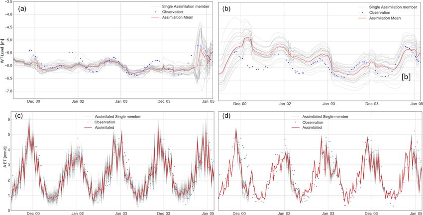
S. Gelsinari et al.: Unsaturated zone model complexity for the assimilation of evapotranspiration rates                                             2267

Table 1. Calibrated parameter values used for the simulations and their coefficient of variation.

                  Model parameter                                                  Configuration 1             Configuration 2        Coefficient
                                                                              UnSAT + MODFLOW              SWAP + MODFLOW          of variation %
                                                                                     homogeneous                  top | bottom
                  Hydraulic conductivity – Ks [mm h−1 ]                                             25                  24 | 41               10
                  Drought stress (reduction) [mm]                                                    –                  −3000                  –
                  Drought stress (no extraction) [mm]                                                –                 −30 000                 –
                  Oxygen stress (reduction) [mm]                                                     –                    −100                 –
                  Oxygen stress (no extraction) [mm]                                                 –                       +5                –
                  Soil porosity [mm3 mm−3 ]                                                       0.35               0.36 | 0.36               –
                  Critical transpiration SM (θ∗ ) [mm3 mm−3 ]                                     0.12                         –               –
                  Residual SM (θr ) [mm3 mm−3 ]                                                  0.03                0.01 | 0.02               –
                  Drainage empirical value [–]                                                    2.50                         –               –
                  Root depth (lr) [mm]                                                           8000                      2900               10
                  Root distribution parameter (Vr) [–]                                             0.5                         –               –
                  MODFLOW Kh [m d−1 ]                                                             10.0                       8.0              10
                  MODFLOW Sy [–]                                                                  0.12                      0.11              10

                                                                               f
To compose the state deviation matrix, the value of x k is                               These lead to the formulation of the Kalman gain as
subtracted from the elements of the state vector as
                                                                                                         PHTk
 f          1,f      f 2,f          f 3,f           f        M,f       f                 Kk =                    ,                                  (16)
Xk     = [x k     − xk xk        − xk xk        − x k · · ·x k     − x k ].        (9)            HPHTk + Rk
   The observation from the CMRSET for the k time step is                                where Rk is the observation error covariance matrix. The
the vector                                                                               Kalman gain transfers the difference between the observed
                                                                                         and simulated AET to the state variables with the updating
y k = AETk ,                                                                   (10)      equation
                                                                                                    i,f               i,f
which is a scalar value because of the choice of matching                                x i,a                         i
                                                                                           k = x k + Kk [y k − ŷ k + vk ],                         (17)
observation and assimilation frequencies. Because of the 8 d
frequency of the observations, the average AET over 8 d sim-                             where vki is a random number with mean 0 and standard de-
ulated by the models is                                                                  viation as the observation error (i.e. 0.2 mm d−1 ).
                                                                                            According to Gelsinari et al. (2020), the state variable up-
             t
 i,f      1X       i,f                                                                   date had to be constrained to preserve numerical stability.
ŷ k =          AETs ,                                                         (11)
          8 s=1                                                                          This was equally true for both models and applies to the WT
                                                                                         levels and SM. A limitation of ±50 % of the prior values
with s being the individual UZM steps. The average over the                              is applied for the SM content of Configuration-1 and, sim-
ensemble population (M) of Eq. (11) reads                                                ilarly, to the pressure head variable of Configuration-2. This
                                                                                         avoids the convergence problem in physically based models
            M
 f       1 X    i,f                                                                      reported in Zhang et al. (2018).
yk =          ŷ .                                                             (12)
         M i=1 k
                                                                                         2.4.1     Ensemble generation
  The matrix for observation–simulation deviation is com-
posed as                                                                                 The generation of a statistically meaningful ensemble, which
                                                                                         preserves the relationship between AET and WT levels ob-
  f         1,f        f   2,f        f   3,f        f       M,f       f
Yk = [ŷ k        − y k ŷ k     − y k ŷ k     − y k · · ·ŷ k    − y k ].    (13)      tained during the calibration, is crucial for the application
                                                                                         of the EnKF (Gelsinari et al., 2020). A number of ensem-
  Combining the matrices calculated above, it is possible to                             ble generation techniques were applied to the two configura-
calculate the background state covariance matrix                                         tions, and a consistent approach for both configurations was
             1  f fT
                                                                                         adopted. The average of the ratios between ensemble skill
PHTk =         X Y                                                             (14)      and ensemble spread, which should tend to 1 over the verifi-
           M −1 k k
                                                                                         cation period, and between √  ensemble skill and mean square
and the observation–simulation error covariance matrix                                   error, which should tend to (M + 1)/2M (Talagrand et al.,
               1  f fT
                                                                                         1997; De Lannoy et al., 2006), were calculated on the mod-
HPHTk =          Y Y .                                                         (15)      elled AET values.
             M −1 k k

https://doi.org/10.5194/hess-25-2261-2021                                                                  Hydrol. Earth Syst. Sci., 25, 2261–2277, 2021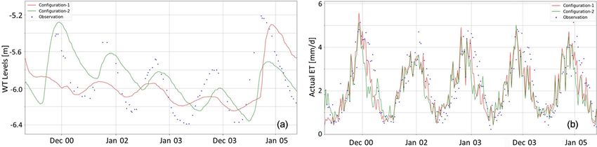
2268              S. Gelsinari et al.: Unsaturated zone model complexity for the assimilation of evapotranspiration rates

   First, a simple perturbation of forcing inputs, by adding         proceed through time. A value of r > 0 implies a positive re-
a random number sampled from Gaussian distributions with             lationship; the closer the value of r is to 1, the stronger and
different standard deviations, as performed by Gelsinari et al.      more accurate the relationship.
(2020), was tested. By perturbing the forcing inputs alone,             The CRPS is a measure to quantify the difference between
the ensemble spread was not reaching appropriate values.             the predicted value and the observed cumulative distribution
Thus, a mixed method involving the perturbation of both in-          in terms of the probabilistic distributions for each time step.
puts and parameters, with the latter perturbed by adding a           The CRPS is calculated, at a specific time step, from the cu-
random number proportionally to the calibrated value, was            mulative distribution function given by the ensemble simu-
applied. For the UZMs, the parameters selected for the per-          lation of the variable of interest x (i.e. AET and WT levels)
turbation were Ks and root depth and for MODFLOW the                 as
saturated Kh and Sy . Initial conditions of WT levels were
                                                                             Z+∞
also perturbed to induce a good spread in the ensemble from
the early stages of the simulation. The Talagrand et al. (1997)      CRPSk =    [P (x)k − P0 (x)k ]2 dx,                        (20)
verification skills were applied to the ensembles generated                     −∞
with the aforementioned approach, and the most adequate en-
                                                                     where P0 is the observation distribution at the time step (k),
sembles for the two configurations were retained. The scores
                                                                     and P (x) is the cumulative distribution function. As the ob-
obtained for the two ratios were comparable to others found
                                                                     servation (x0 ) is usually a single value, P0 is formulated as
in the literature (e.g. De Lannoy et al., 2006; Pauwels and De
                                                                     P0 = H (x − x0 ), H being the Heaviside function. The CRPS
Lannoy, 2009; Gelsinari et al., 2020). These ensembles are
                                                                     is applied to reinforce the value of the result as it is specif-
defined as the open loop, which represents the “prior” distri-
                                                                     ically designed to assess probabilistic simulations and is in-
bution. After applying the filter, the resulting distribution is
                                                                     creasingly being used in hydrologic ensemble simulations.
called the assimilation run and represents the “posterior”.
                                                                     The reasons are that it intrinsically weighs errors by assign-
2.5    Verification skills                                           ing a lower weight to the largest residuals (Schneider et al.,
                                                                     2020), thus accounting for observations that in other cases
In this section, the results for the open loop and assimilation      are defined as outliers. Therefore, it is the preferable mea-
runs are assessed. This is conducted by analysing the error          sure in determining the error in forecasting models since it is
between the prediction of the model and the observations.            more robust to outliers, producing a more representative re-
The common error metrics used to assess the overall errors           sult. Note that a value of the CRPS of zero is only possible in
in these models are the root mean square error (RMSE), the           the case of a perfect deterministic forecast. Thus, the lower
Pearson correlation coefficient (r), and the continuous ranked       the value of the CRPS, the better the model performance.
probability score (CRPS) (Hersbach, 2000).                              This is calculated over the entire simulation period, and
   The RMSE and r are defined as                                     the average CRPS is defined as
           v                                                                       L
           u L
           u1 X                                                                 1X
                                                                     CRPS =           CRPSk ,                                   (21)
RMSE = t            (ok − fk )2 ,                          (18)                 L k=1
              L k=1
                                                                     where L is the number of observations. This permits an anal-
where ok is the observations, fk is the modelled variables at        ysis of the measures and a comparison of the RMSE and the
time step k, and L is the size of the data set. The RMSE is          CRPS. In this experiment, the models are naturally stochastic
an important metric which measures the square of the differ-         processes, allowing the CRPS to produce a more representa-
ence in the errors and is presented to convey a possible broad       tive value and robust measure for the errors compared to the
overall error between the observations and the model. A dis-         RMSE. In conclusion of this section, all three measures will
advantage of RSME is the excessive weight of large outliers.         be used to assess the performance of the filter.
   The next component for analysing the performance in ver-
ifying the results is the Pearson correlation coefficient to un-
derstand the relationship between the observed values and            3     Results and discussion
the predicted model values. The Pearson correlation coeffi-
cient (r) is defined as                                              3.1    Deterministic runs
           PL                                                        During the calibration with the PSO, the dynamics of the
              k=1 (ok
                   − o)(fk − f )
r = qP                                 .                     (19)    parameter optimisation algorithm was monitored, showing
       L             2·
                        PL           2
             (o
          k=1 k − o)        (f
                         k=1 k  − f )                                that the MODFLOW saturated hydraulic conductivity (Kh )
                                                                     had a consistent tendency towards high values (100 m d−1 or
   In particular, this investigates the strength of the linear re-   higher) in order to minimise Eq. (4). This was interpreted
lationship between the predicted and observed values as they         as an effect of the AET component on the objective function,

Hydrol. Earth Syst. Sci., 25, 2261–2277, 2021                                         https://doi.org/10.5194/hess-25-2261-2021
S. Gelsinari et al.: Unsaturated zone model complexity for the assimilation of evapotranspiration rates 2269
Table 2. Results for the calibrated runs. Configuration-2. In particular, Configuration-2, being physi-
cally based, underestimates the simulated AET for the South-
Variable Configuration RMSE r ern Hemisphere late summer and early autumn, as shown in
WT 1 0.230 [m] 0.790 Fig. 4b. In this period, the soil water content is low (Fig. 5d),
Levels 2 0.360 [m] 0.400 and the roots take up water directly from groundwater. This
SM 1 0.049 [mm3 mm−3 ] 0.410 can be interpreted as an effect of the coupling to the ground-
Upper 2 0.045 [mm3 mm−3 ] 0.610 water model. Configuration-1, which is conceptually based,
SM 1 0.085 [mm3 mm−3 ] 0.592 with a rooting depth of 8.0 m, is able to extract water directly
Lower 2 0.018 [mm3 mm−3 ] 0.850 from the water table and immediately transforms it into AET.
AET 1 0.791 [mm d−1 ] 0.811 Configuration-2, with a rooting depth of 2.9 m, achieves this
2 0.870 [mm d−1 ] 0.788 by reducing the pressure head along the soil column. Thus
water has to flow across a part of the unsaturated zone be-
fore becoming available for direct plant transpiration, reduc-
ing the rapid response of the model to the forcing inputs.
which was causing the UZMs to transpire water directly from This also explains the lag in the WT dynamics previously de-
the WT to compensate for the low AET values. The bound- scribed. Another possible reason for the underestimation of
ary conditions for the groundwater model were thus modified AET is the two oxygen stress parameters that reduce transpi-
by imposing a constant head boundary with shallower WT ration in conditions close to saturation (Table 1). These pa-
depth, which maintained Kh at a plausible order of magni- rameters are calibrated and kept constant during the simula-
tude (Table 2). tion period. Configuration-2 has shown to be highly sensitive
With the calibration technique proposed in Sect. 2.3, the to these parameters, while Configuration-1 does not include
coupled models were able to simultaneously reproduce the this process.
dynamics of both the WT and ET for the two configura-
tions. Configuration-1 performs better overall in the repre- 3.2 Ensemble simulations
sentation of the WT dynamics with a RMSE of 0.23 m, while
the RMSE of Configuration-2 is slightly larger, being 0.36 m. The generation of the ensemble was found to be a key step of
Configuration-1 also shows a higher correlation coefficient the method. The simple perturbation of forcing inputs was
(0.790 vs. 0.400) for the WT. Configuration-1 shows a lower not able to generate a sufficiently broad ensemble spread,
temporal variability than Configuration-2, but the latter bet- particularly for Configuration-2. For both configurations, the
ter matches the temporal evolution of the WT. There is a time combined perturbation of parameters and forcing inputs in-
lag between groundwater observations and model WT fluc- duced more accurate ensembles, in accordance with the en-
tuation for Configuration-2, which also explains the higher semble validation skills calculated on the first year of the
RMSE and lower correlation. This lag may be induced by data set, excluding the 10 first time steps to avoid the in-
preferential flow that the Richards equation does not account fluence of the initial conditions; the validation is thus ap-
for or by a slower response of the WT to the meteorological plied from the 10th to the 45th time step. For the meteoro-
input that is discussed later in this section. logical data, the best ensembles are obtained by perturbing
The soil heterogeneity is represented differently by the two the input with a random number sampled from a Gaussian
configurations. Configuration-2, which is physically based, distribution having a standard deviation proportional to the
can represent the heterogeneity of the soil column, as shown value of the forcing inputs (i.e. 50 % for Configuration-1 and
in Fig. 5d, where a sharp variation of the SM content 10 % for Configuration-2). For parameters, the last column
at 1.7 m depth is caused by the different soil parameters. of Table 1 lists the coefficient of variation. Additionally, for
Configuration-1 has no ability to explicitly account for du- Configuration-2, Sy has a lower limit of 0.1 to preserve nu-
plex soil; thus the soil profile does not show sharp variations merical stability of the coupled models.
of the water content. However, it can account for the decay of In the case of Configuration-1, which is conceptually
the hydraulic conductivity along the soil column. Because of based, the WT level spread of the open-loop ensemble is
these reasons, the modelled SM from Configuration-2 shows consistently covering the observations (Fig. 6a). The mean
a good agreement with the observations, especially in the of the ensemble is close to the observations but does not
lower soil (Fig. 5f). Configuration-1 has a low SM RMSE follow the seasonal variability appropriately. The associated
(0.049 mm3 mm−3 ) and a Pearson correlation coefficient r spread of the AET for Configuration-1 is wider than that of
of 0.41 for the upper soil (b), but the resulting SM is con- Configuration-2. More specifically, the latter is narrow dur-
sistently below the observed values in the bottom soil (panel ing wet periods (i.e. April to November) and becomes wider
c), with an RMSE of 0.137 mm3 mm−3 . Both configurations for the dry period (Fig. 6c and d). A similar effect, with a
report a higher correlation for the lower soil. larger magnitude, was reported during the ensemble genera-
For AET, Configuration-1 yields good results with a tion phase and led to the perturbation of both the meteoro-
lower RMSE and similar correlation when compared to logical inputs and the parameters, as explained in Sect. 2.4.1.
https://doi.org/10.5194/hess-25-2261-2021 Hydrol. Earth Syst. Sci., 25, 2261–2277, 20212270 S. Gelsinari et al.: Unsaturated zone model complexity for the assimilation of evapotranspiration rates
Figure 4. Observed and modelled (a) WT fluctuations and (b) AET after calibration.
The spread of the WT levels for Configuration-2 (see is not reflected in a higher modelled AET. The reason for
Fig. 6b) covers the WT observations for most of the simu- this is the behaviour of the SWAP vegetation parameter oxy-
lations and is wider than for Configuration-1. The mean rep- gen stress. The filter is increasing the pressure head of the
resents the amplitude of the seasonal fluctuations better as system, in an attempt to provide more water to transpire, but
compared to Configuration-1 but leads to a shallower WT as the actual transpiration from the plant is hindered by SWAP,
a result of the perturbation of the forcing inputs. which recognises the soil to be too saturated for the plant
Table 3 summarises the RMSE, r, and CRPS values for to transpire. The EnKF then causes the WT to rise and in-
AET, WT levels, and SM contents (upper and lower soil lay- creases the amount of recharge entering the groundwater.
ers) and compares the results of the assimilation run to the When the observed AET is lower than the simulations, the
open loop. The table allows for a quick comparison between filter reduces the pressure head, and the model allows the
the results given by the RMSE, standardly used and under- plant to transpire. Therefore, in the two time steps after this
stood across the modelling community, and the CRPS aver- effect, the modelled AET is higher than the observation, after
aged over the simulation period (i.e. CRPS), which allows which this phenomenon disappears. This artefact is not seen
for an appropriate and representative analysis of the ensem- in Configuration-1 as the oxygen stress is not accounted for.
ble distributions. For both configurations, the AET assimi- In Fig. 8, the single bars represent the CRPSk com-
lation slightly decreases the RMSE and the CRPS and im- puted for each time the observations (WT levels above,
proves the correlations. In particular, the RMSE of AET for AET below) are available over the entire simulation pe-
Configuration-1 reduces from 0.76 mm d−1 for the open loop riod. For this reason, the length of these data sets is dif-
to 0.73 mm d−1 . The RMSE of AET for Configuration-2 re- ferent, as the CMRSET observations’ temporal interval is
duces from 0.83 mm d−1 for the open loop to 0.81 mm d−1 . 8 d, while the WT levels’ observations are more infrequent
A similar pattern is observed for the CRPS, with the rel- and present gaps. Generally, lower CRPS values are seen in
ative percentage change improvements varying from 4.3 % Configuration-1 for both WT levels and AET. CRPS values
to 6.1 %. In this case, the CRPS reinforces the relevance of for the WT level are substantially reduced in the first part of
the RMSE results. The correlation also improves, although the simulation for both configurations, with Configuration-1
marginally, for both configurations (i.e. +0.01). However, performing particularly well between August 2002 through
these are non-trivial results as the data assimilation, through July 2003 and in reducing the prior errors around the end
the EnKF, is designed to only improve the model states. of 2004. Analysing the CRPS values for AET (see Fig. 8c),
Therefore, the observed reduction in AET errors suggests in most cases the assimilation improves the CRPS values,
that the model states (i.e. WT, SM) updated by the filter are with the exemption of the middle of 2004. This is also seen
contributing to better modelling of other hydrological quan- in Fig. 7 when the assimilation fails to reduce the AET in
tities (e.g. AET). the winter of 2004. For Configuration-2, the WT level CRPS
In particular there are instances in Configuration-2 where starts with higher values, and apart from the spikes of 2001
the assimilation is not able to improve AET in the first quarter (discussed earlier), it presents continuous, constant improve-
of 2001 and, to a lesser extent, at the beginning of 2003. This ments, outperforming Configuration-1 in the last part of the
causes poorer WT simulations’ performances during these simulation. This pattern is similarly observed for the CRPS
periods, as seen in Fig. 7b and highlighted by the higher val- calculated for AET.
ues in Fig. 8b. Here, the filter is trying to increase the amount For both configurations, the assimilation improves the
of water in the system to match the higher assimilated ob- RMSE and CRPS when compared to the open loop runs.
servation, which is a correct application of the methodol- The best results are obtained for Configuration-1, showing
ogy. Thus, the WT is made shallower by the filter, but this a RMSE of 0.236 m with a 15 % error reduction compared to
Hydrol. Earth Syst. Sci., 25, 2261–2277, 2021 https://doi.org/10.5194/hess-25-2261-2021S. Gelsinari et al.: Unsaturated zone model complexity for the assimilation of evapotranspiration rates 2271 Figure 5. Temporal evolution of the SM contents and WT levels. Panels (a, d) show the entire modelled column, including the fluctuation of the WT (i.e. the dark blue area). Panels (b, e) represent the modelled and observed water content for the upper soil (averaged over 0–300 mm depth). Panels (c, f) show these results for the lower soil (averaged over the interval 1500–1800 mm depth). Figure 6. WT levels and AET and spread of the open-loop ensembles for Configuration-1 (a, c) and Configuration-2 (b, d). https://doi.org/10.5194/hess-25-2261-2021 Hydrol. Earth Syst. Sci., 25, 2261–2277, 2021
2272               S. Gelsinari et al.: Unsaturated zone model complexity for the assimilation of evapotranspiration rates

Figure 7. WT levels and AET and spread of the assimilation run for Configuration-1 (a, c) and Configuration-2 (b, d).

Table 3. RMSE, correlation and CRPS for three variables between the open loop and the assimilation.

  Config.   Type                      AET                        WT levels                SM upper soil              SM lower soil
                            RMSE          r   CRPS     RMSE            r     CRPS    RMSE          r   CRPS    RMSE          r   CRPS
  1         Open-loop        0.760    0.820    0.541     0.280     0.730     0.161    0.045    0.497   0.204     0.102   0.468   0.078
            Assimilation     0.730    0.830    0.508     0.236     0.734     0.134    0.044    0.498   0.206     0.098   0.428   0.077
  2         Open-loop        0.830    0.810    0.624     0.626     0.880     0.426    0.041    0.888   0.037     0.019   0.940   0.013
            Assimilation     0.810    0.820    0.597     0.307     0.675     0.229    0.042    0.864   0.036     0.015   0.900   0.012

the open loop; this result is confirmed by the CRPS of 0.134               0.102 mm3 mm−3 for the lower soil. In the latter, the simu-
(error reduction of 16 %). Configuration-2 resulted in a sub-              lated water contents are consistently lower than the observa-
stantial RMSE reduction of 38.9 % as compared to the open                  tions. This is mainly due to the model’s inability to represent
loop. The magnitude of these improvements is corroborated                  capillary rise. The assimilation only marginally improved the
by the CRPS, with a value after the assimilation of 0.229                  SM content, with slightly better results for the bottom part of
from the prior of 0.426, which translates to an improvement                the soil, where the RMSE was reduced to 0.098 mm3 mm−3 .
of around 46 %. However, RMSE and CRPS values (0.307                       The open loop of Configuration-2 has a lower RMSE, 0.041
and 0.229 m, respectively) are still higher in Configuration-1             and 0.017 mm3 mm−3 for the top and bottom part of the soil,
than in Configuration-2. Apart from the oxygen stress arte-                respectively. However, it slightly overestimates the SM con-
facts explained above, the assimilation run of Configuration-              tent for the entire column. This is consistent with the shal-
2 is consistently better than the open loop. This is not always            lower WT (i.e. more water in the system) observed for the
the case for Configuration-1, where the open loop was al-                  WT levels in the open loop (Fig. 6d). The assimilation did
ready performing well. The correlation remains largely un-                 not improve the top layer SM content, with an RMSE of
changed for Configuration-1 and reduces for Configuration-                 0.042 mm3 mm−3 . However, effects of the assimilation are
2, mainly due to the updates during the first quarter of 2001              seen for the SM content of the lower soil, for which the best
and beginning of 2003.                                                     results are obtained (i.e. 0.015). For SM, the CRPS is unable
   For SM, the results are reported in Table 3, divided into               to show significant variations and does not add valuable in-
the upper and lower soil. The open loop of Configuration-1                 formation. Although the improvements for SM are limited
presents a RMSE of 0.045 mm3 mm−3 for the upper soil and                   and cannot be considered conclusive, the feasibility for this

Hydrol. Earth Syst. Sci., 25, 2261–2277, 2021                                               https://doi.org/10.5194/hess-25-2261-2021
S. Gelsinari et al.: Unsaturated zone model complexity for the assimilation of evapotranspiration rates 2273
Figure 8. CRPS WT levels and AET for Configuration-1 (a, c) and Configuration-2 (b, d).
framework of updating the entire soil column is a positive The most important findings can be summarised as fol-
result of the assimilation of AET rates, as opposed to the as- lows:
similation of remotely sensed SM values. The latter usually – Calibration. This study shows the need to calibrate the
results in stronger updates in the upper parts of the soil be- model using a multi-objective function, with normalised
cause of the reduced correlation between the SM contents in components of water table (WT) and AET. In this way,
the upper and deeper parts of the soil column (Pipunic et al., both configurations represent the WT-AET dynamics
2014). and are thus able to benefit from the assimilation of AET
Generally, these results consolidate the synthetic approach observations.
in Gelsinari et al. (2020) and further confirm that the assim-
ilation framework is not only able to update and improve – Configuration-1. The assimilation of AET values
the WT level, which is a prognostic variable of the coupled through the ensemble Kalman filter (EnKF) using a con-
models, but also the modelled AET and consequently the ceptual UZM produced the best results for the prognos-
recharge to the WT. In addition, albeit marginally, the filter tic variable WT levels and the diagnostic fluxes of AET.
improves the unsaturated zone state variables regardless of SM values were updated in both the upper and lower
the manner in which the SM content is calculated (volumet- parts of the soil column, although only to a minor extent.
ric SM or pressure head). In addition, because of the model conceptualisation, the
mismatch in the lower part of the soil is considerably
larger than for Configuration-2. The reduced number
4 Conclusions of parameters of this configuration allows for a simpler
calibration, which is able to represent the WT dynamics.
This study validates the assimilation of the satellite-based ac- Similarly, the generation of an appropriate ensemble is
tual evapotranspiration (AET) data set (CMRSET) into two more straightforward, mostly due to the model concep-
unsaturated zone models (UZM) coupled to MODFLOW. tualisation, which allows the WT to respond quickly to
The two UZMs form two configurations, one using a con- direct root water extraction by transpiration.
ceptual water balance model (UnSAT) and the other using
a physically based agro-hydrological model (SWAP). These – Configuration-2. The AET assimilation into a physi-
configurations are applied to a semi-arid pine plantation in cally based UZM, based on the Richards equation, pro-
the south-east of South Australia, where the WT is within duced the largest improvements to the WT levels, with a
reach of the trees’ root system. better representation of the soil heterogeneity. Improve-
ments to AET fluxes were similar for Configuration-1.
https://doi.org/10.5194/hess-25-2261-2021 Hydrol. Earth Syst. Sci., 25, 2261–2277, 20212274 S. Gelsinari et al.: Unsaturated zone model complexity for the assimilation of evapotranspiration rates
For SM, the impact of the assimilation algorithm was Data availability. Model forcing inputs, assimilated evapotranspi-
small, with a positive update for the lower soil lay- ration from CMRSET, and experiment results are available at
ers and a negative update for the upper layers. Here, https://doi.org/10.6084/m9.figshare.14430998 (Gelsinari, 2021).
the calibration involved a larger number of parameters
and produced a good representation of the SM dynam-
ics. However, due to the non-linearity introduced with Author contributions. SG performed the modelling work and wrote
the coupling, errors in the WT levels and AET fluxes the manuscript. VRNP supervised the implementation of the EnK,
ED supervised the implementation of the UnSAT model, JvD su-
are higher. In addition, the ensemble generation is con-
pervised the implementation and coupling of the SWAP model,
strained by the high model parameterisation, making it
NFY contributed to the results analysis, and RD supervised the
more difficult to produce an appropriate ensemble that entire project. All co-authors provided input to the writing of the
preserves the AET–WT relationship. manuscript.
– AET information. The updating of the entire soil column Competing interests. The authors declare that they have no conflict
is an advantage of the assimilation of remotely sensed of interest.
AET over satellite SM retrievals. AET rates express the
moisture status of the entire root zone. Thus, assimilat-
ing AET has the potential to overcome the SM assimi- Special issue statement. This article is part of the special issue
lation tendency to produce stronger updates in the most “Data acquisition and modelling of hydrological, hydrogeological
superficial part of the soil because of the reduced corre- and ecohydrological processes in arid and semi-arid regions”. It is
lation between the upper and lower SM contents. This not associated with a conference.
experiment only showed the feasibility of the proposed
assimilation framework to improve SM contents. Pre-
liminary results indicated that Configuration-2 is pre- Acknowledgements. Simone Gelsinari acknowledges the financial
ferred to conduct more experiments in order to quantify support by the Faculty of Engineering at Monash University
the significance of the SM updates. through the Graduate Research International Travel Award and
thanks the chair group of Hydrology and Quantitative Water Man-
agement at Wageningen University & Research for the support dur-
In conclusion, the numerical experiment explored the ing his visit. Simone Gelsinari also thanks Karina Gutierrez Jurado
added value of AET information for constraining unobserv- for her support and suggestions during the preparation of this paper.
able estimates (i.e. net recharge) calculated by hydrogeolog-
ical models. Improving the AET fluxes led to better recharge
estimates. Thus, as recharge is a key quantity driving the WT Financial support. This research has been supported by the Com-
dynamics, the link between AET and WT in the model is monwealth Scientific and Industrial Research Organisation (Effec-
strengthened. It was shown that it is possible to use either tive Floodplain Management Project).
a conceptual or a physically based UZM in the assimilation
of satellite-based AET estimates to inform hydrogeological
models. The assimilation results have been quantified using Review statement. This paper was edited by Harrie-Jan Hendricks
standard metrics, such as RMSE and r, and reinforced by Franssen and reviewed by Manuela Girotto and two anonymous ref-
calculating the CRPS, which is a specifically designed met- erees.
ric for ensemble simulations. The CRPS is applied as it is a
measure to determine a more representative error, since it is
more robust in accounting for uncertainty in stochastic mod-
els. The findings indicate that a simple conceptual model may References
be sufficient for this purpose; thus using one configuration
over the other should be motivated by the specific purpose of Bakker, M., Post, V., Langevin, C. D., Hughes, J. D., White, J. T.,
the simulation and the information available. Starn, J. J., and Fienen, M. N.: Scripting MODFLOW Model De-
This study contributes to unlocking the potential of using velopment Using Python and FloPy, Groundwater, 54, 733–739,
AET observations to inform hydrological models, with the https://doi.org/10.1111/gwat.12413, 2016.
Banks, E. W., Brunner, P., and Simmons, C. T.: Vegetation con-
aim of reducing the uncertainty in the outputs, and it repre-
trols on variably saturated processes between surface water and
sents a step towards the use of satellite-based AET retrievals
groundwater and their impact on the state of connection, Water
for water resources management. For future applications at Resour. Res., 47, 1–14, https://doi.org/10.1029/2011WR010544,
larger scales, more research is to be conducted in areas with 2011.
different groundwater, vegetation, and soil conditions, with Batelaan, O. and De Smedt, F.: GIS-based recharge estimation
the intent of prioritising regions where the AET assimilation by coupling surface-subsurface water balances, J. Hydrol., 337,
is more effective. 337–355, https://doi.org/10.1016/j.jhydrol.2007.02.001, 2007.
Hydrol. Earth Syst. Sci., 25, 2261–2277, 2021 https://doi.org/10.5194/hess-25-2261-2021You can also read