Quantifying fugitive gas emissions from an oil sands tailings pond with open-path Fourier transform infrared measurements
←
→
Page content transcription
If your browser does not render page correctly, please read the page content below

Atmos. Meas. Tech., 14, 945–959, 2021
https://doi.org/10.5194/amt-14-945-2021
© Author(s) 2021. This work is distributed under
the Creative Commons Attribution 4.0 License.

Quantifying fugitive gas emissions from an oil sands tailings pond
with open-path Fourier transform infrared measurements
Yuan You1,a , Samar G. Moussa1 , Lucas Zhang2 , Long Fu2 , James Beck3 , and Ralf M. Staebler1
1 AirQuality Research Division, Environment and Climate Change Canada (ECCC), Toronto, M3H 5T4, Canada
2 Alberta Environment and Parks, Edmonton, T5J, 5C6, Canada
3 Suncor Energy Inc., Calgary, T2P 3Y7, Canada
a now at: Department of Physics, University of Toronto, Toronto, M5S 1A7, Canada

Correspondence: Ralf M. Staebler (ralf.staebler@canada.ca)

Received: 26 June 2020 – Discussion started: 6 August 2020
Revised: 3 November 2020 – Accepted: 13 November 2020 – Published: 8 February 2021

Abstract. Fugitive emissions from tailings ponds contribute           1   Introduction
significantly to facility emissions in the Alberta oil sands,
but details on chemical emission profiles and the temporal
and spatial variability of emissions to the atmosphere are            Tailings from the oil sands industrial processes in Alberta’s
sparse, since flux measurement techniques applied for com-            Athabasca oil sands consist of a mixture of water, sand, non-
pliance monitoring have their limitations. In this study, open-       recovered bitumen, and additives from the bitumen extrac-
path Fourier transform infrared spectroscopy was evaluated            tion processes (Small et al., 2015). These tailings are de-
as a potential alternative method for quantifying spatially           posited into large engineered tailings ponds on site. Sep-
representative fluxes for various pollutants (methane, ammo-          aration of processed water from remaining tailings occurs
nia, and alkanes) from a particular pond, using vertical-flux-        continuously in the tailings pond, and the processed water
gradient and inverse-dispersion methods. Gradient fluxes              is recycled (Canada’s oil sands tailings ponds: https://www.
of methane averaged 4.3 g m−2 d−1 but were 44 % lower                 canadasoilsands.ca/en/explore-topics/tailings-ponds, last ac-
than nearby eddy covariance measurements, while inverse-              cess: 29 September 2019). The total liquid surface area
dispersion fluxes agreed to within 30 %. With the gradient            covered by tailings ponds in the Athabasca oil sands was
fluxes method, significant NH3 emission fluxes were ob-               103 km2 in 2016 and continues to grow (Alberta Environ-
served (0.05 g m−2 d−1 , 42 t yr−1 ), and total alkane fluxes         ment and Parks, 2016).
were estimated to be 1.05 g m−2 d−1 (881 t yr−1 ), represent-            Emissions to the atmosphere from tailings ponds include
ing 9.6 % of the facility emissions.                                  methane (CH4 ), carbon dioxide (CO2 ), reduced sulfur com-
                                                                      pounds, volatile organic compounds (VOCs), and polycyclic
                                                                      aromatic hydrocarbons (PAHs) (Siddique et al., 2007; Simp-
                                                                      son et al., 2010; Yeh et al., 2010; Siddique et al., 2011, 2012;
Copyright statement. The works published in this journal are          Galarneau et al., 2014; Small et al., 2015; Bari and Kindzier-
distributed under the Creative Commons Attribution 4.0 License.       ski, 2018; Zhang et al., 2019; Foght et al., 2017; Penner and
This license does not affect the Crown copyright work, which          Foght, 2010). Emissions from tailings ponds vary with pond
is re-usable under the Open Government Licence (OGL). The             conditions, such as pond age and solvent additives in the
Creative Commons Attribution 4.0 License and the OGL are
                                                                      ponds, and can contribute significantly to total facility emis-
interoperable and do not conflict with, reduce or limit each other.
                                                                      sions (Small et al., 2015).
© Crown copyright 2021                                                   Very few studies focusing on emissions of air pollutants
                                                                      from tailings ponds have been published (Galarneau et al.,
                                                                      2014; Small et al., 2015; Zhang et al., 2019). Compounds
                                                                      of particular interest include alkanes and ammonia (NH3 ).

Published by Copernicus Publications on behalf of the European Geosciences Union.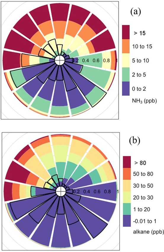
946                                                        Y. You et al.: Tailings pond fugitive emissions quantified by FTIR

Alkanes are part of the solvents used in the extraction pro-       etable farm in Australia using an OP-FTIR system with two
cess (Small et al., 2015) and can dominate VOCs emissions          paths vertically separated by 0.5 m on average. At the same
from oil sands facilities (Li et al., 2017). Previously reported   vegetable farm, Bai et al. (2019) measured emission rates of
VOCs emissions by facilities had large uncertainties, espe-        N2 O using flux chambers and OP-FTIR slant path configu-
cially from fugitive sources, due to limitations of the meth-      ration with flux-gradient methods and showed a large vari-
ods used to estimate emissions for compliance monitoring           ation of the ratio of N2 O fluxes with these two measure-
purposes (Li et al., 2017). VOCs in the atmosphere are im-         ments. Inverse-dispersion models have also been applied to
portant because of their effects on ambient ozone and sec-         OP-FTIR measurements to quantify emission rates in previ-
ondary aerosol formation (Field et al., 2015; Kroll and Se-        ous studies (Flesch et al., 2004, 2005; Bai et al., 2014; Hu et
infeld, 2008). Emissions of NH3 from tailings ponds to the         al., 2016; Shonkwiler and Ham, 2018).
atmosphere have not been published, although NH3 has been             Longer continuous coverage with a greater height differ-
observed in the oil sands region (Bytnerowicz et al., 2010;        ence between paths is one distinguishing feature of this study
Whaley et al., 2018). NH3 emissions have important environ-        compared to previous research. The motivation of this work
mental implications, such as forming atmospheric aerosols          is to quantify emission rates of pollutants from one specific
with sulfuric acid (Kürten, et al., 2016) and affecting nitrogen   tailings pond by combining OP-FTIR measurements with
deposition in the ecosystem (Makar, et al., 2018). This infor-     micrometeorological methods. Emissions of CH4 , NH3 , and
mation is important for model simulations of critical loads of     total alkanes as well as a comparison of gradient and inverse-
acidifying deposition in the ecosystem (Makar, et al., 2018).      dispersion methods are presented in this study.
This field measurement project provided a great opportunity
to continuously measure and to quantify tailings pond emis-
sions over more than a month, especially for NH3 and total         2     Open-path FTIR field measurements and methods
alkanes.                                                                 for deriving fluxes
   Open-path Fourier transform infrared (OP-FTIR) spec-
                                                                   2.1    Site and measurement setup
troscopy has been considered a good candidate for an alter-
native method to monitor fugitive emissions from industrial        The main site of this study was on the south shore of
or hazardous waste area sources, since the method is non-          Suncor Pond 2/3 (Fig. 1; 56◦ 590 0.9000 N, 111◦ 300 30.3000 W,
intrusive, integrates over long path lengths, and has the abil-    305 m a.s.l.). Sensible heat and momentum fluxes were mea-
ity to quantify several different gases of interest simultane-     sured on a mobile tower with sonic anemometers (model
ously and continuously (Marshall et al., 1994), without sam-       CSAT3, Campbell Scientific, USA) at 8, 18, and 32 m above
ple line issues. It has previously been used to quantify mole      ground. Vertical gradients of gaseous pollutant mole frac-
fractions of various air pollutants from different sources such    tions were measured by drawing air from 8, 18, and 32 m
as forest fires (Griffith et al., 1991; Yokelson et al., 1996,     on the tower to instrumentation housed in a trailer on the
1997; Goode et al., 1999; Yokelson, 1999; Yokelson et al.,         ground. A fourth sample inlet at 4 m was on the roof of the
2007; Burling et al., 2010; Johnson et al., 2010; Akagi et al.,    main trailer beside the mobile tower. CH4 and H2 O mole
2013; Yokelson et al., 2013; Akagi et al., 2014; Paton-Walsh       fractions at these four levels were measured sequentially by
et al., 2014; Smith et al., 2014), volcanoes (Horrocks et al.,     cavity ring-down spectroscopy (CRDS) (model G2204, Pi-
1999; Oppenheimer and Kyle, 2008), industrial sites (Wu et         carro, USA). CH4 mole fractions at 4 m were used to cal-
al., 1995), harbors (Wiacek et al., 2018), and road vehicles       ibrate the mole fraction from OP-FTIR retrievals. At 18 m,
(Bradley et al., 2000; Grutter et al., 2003; You et al., 2017).    CH4 mole fractions were also measured by another CRDS
OP-FTIR measurements with vertically separated paths have          (model G2311-f, Picarro, USA) at 10 Hz, to be combined
previously been conducted to derive the emission rate of air       with sonic anemometer measurements to calculate the eddy
pollutants. Schäfer et al. (2012) deployed two OP-FTIR spec-       covariance (EC) flux. Meteorological parameters including
trometers with parallel paths 2.2 m vertically apart at a grass-   temperature and relative humidity (RH) were measured at
land in Fuhrberg, Germany, to measure nitrous oxide (N2 O)         the same three levels on the tower and 1 m above ground.
emissions with a flux-gradient method and showed the calcu-        A propeller anemometer (model 05103-10, Campbell Sci-
lated flux is comparable to the chamber measurements at the        entific, USA) on the roof of the main trailer at 4 m above
same grassland. Flesch et al. (2016) deployed OP-FTIR mea-         ground provided an additional measurement of wind speed
surement with one spectrometer and two paths vertically sep-       and direction. Measurements were conducted from 28 July
arated by about 1 m on average (slant path configuration) at       to 5 September 2017. The FTIR spectrometer was located
a cattle field in Alberta, Canada. They derived emission rates     10 m to the east of the flux tower, and the paths were along
of N2 O and NH3 by flux-gradient and inverse-dispersion            the south shore of the pond. This paper focuses on derived
methods, demonstrating the capability of OP-FTIR systems           fluxes from the measurement of OP-FTIR. Other experimen-
to measure emission rates of N2 O and NH3 . Following the          tal details of the project can be found in You et al. (2020).
flux-gradient method in Flesch et al. (2016), Bai et al. (2018)
measured the flux of N2 O, NH3 , CH4 , and CO2 from a veg-

Atmos. Meas. Tech., 14, 945–959, 2021                                                https://doi.org/10.5194/amt-14-945-2021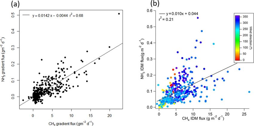
Y. You et al.: Tailings pond fugitive emissions quantified by FTIR                                                                        947

Figure 1. Map of the site: open-path FTIR on the south shore marked in red, open-path FTIR of Alberta Environment and Parks (AEP) on
the north shore marked in yellow, and the outfall on the west side. The colored rose plot shows 50 % and 80 % contribution distances for
eddy covariance fluxes at 18 m using the Flux Footprint Prediction (FFP) model (Kljun et al., 2015). The unit of contribution distances is in
meters. The white circle labels the 2.3 km distance from the main site, equivalent to 100 times the height of the highest point of the top FTIR
path. This figure is adapted from You et al. (2020), Fig. 1.

2.2   Open-path Fourier transform infrared                                ing the 5-week study due to reflector deterioration, presum-
      spectrometer (OP-FTIR) system                                       ably mostly due to impaction by particulate matter. This re-
                                                                          flector deterioration also decreased the signal-to-noise ratio
                                                                          by around 67 %, based on spectral retrievals for CH4 , but did
The FTIR measurements were taken with a commercial Open                   not affect the mean mole fractions measured.
Path FTIR Spectrometer (Open Path Air Monitoring System                      In this study, spectra were measured at a resolution of
(OPS), Bruker, Germany), which was set up at 1.7 m above                  0.5 cm−1 with 250 scans co-added to increase signal-to-noise
the ground in a trailer. The infrared source is an air-cooled             ratio, resulting in roughly a 1 min temporal resolution. Stray
Globar. The emitted radiation is directed through the inter-              light spectra were recorded regularly by pointing the spec-
ferometer where it is modulated, travels along the measure-               trometer away from the retroreflectors. This stray light spec-
ment path (200 m horizontal distance) to a retroreflector ar-             trum accounts for radiation back to the detector from internal
ray that reflects the radiation, travels back to the spectrome-           reflections inside the spectrometer, i.e., not from the retrore-
ter, and enters a Stirling-cooled mercury cadmium telluride               flector array, and was subtracted from all the measurement
(MCT) detector (monostatic configuration). Three retrore-                 spectra before performing further analysis.
flectors were employed in this study: one near ground level                  Spectral fitting was performed with OPUS_RS (Bruker),
(1 m) on a tripod and two at higher elevations on basket lifts,           which uses a non-linear curve-fitting algorithm (You et al.,
resulting in heights of reflectors of approximately 1, 11, and            2017). Spectral windows and interference gases for each gas
23 m above ground. Three paths with these three retroreflec-              (Table 1) were determined by optimizing capture of the ab-
tors are referred to as bottom, middle, and top paths. The                sorption features while minimizing interferences. To further
bottom retroreflector was approximately twice the size of the             improve fittings, baselines were optimized through either lin-
upper two (59 vs. 30 reflector cubes). All retroreflectors were           ear or Gaussian fits under given spectral windows and inter-
cleaned with an alcohol solution once during the study, and               fering gases. For CH4 and CO2 , temperature-dependent ref-
the bottom mirror was rinsed with de-ionized water three                  erence files were used for fitting and retrieving mole frac-
times. Return signal strength decreased by around 65 % dur-

https://doi.org/10.5194/amt-14-945-2021                                                         Atmos. Meas. Tech., 14, 945–959, 2021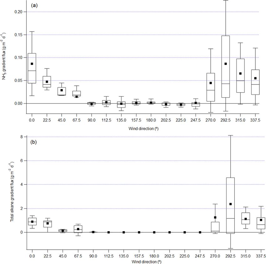
948                                                                           Y. You et al.: Tailings pond fugitive emissions quantified by FTIR

Table 1. Spectral windows of OP-FTIR spectra for retrieving mole fractions of pollutants in this study.

         Pollutant               Chemical             Spectral       Interference gases                             Threshold        Detection        Paths
         name                    formula              window                                                       correlation       limitc
                                                      (cm−1 )                                                     coefficienta
         Methane                 CH4              3006–3021          H2 O                                                  0.95      1.1 ppb          All three
         Ammonia                 NH3                 957–973         H2 O, CO2                                               0.3     1.1 ppb          All three
         Methanol                CH3 OH           1020–1040          H2 O, NH3 , O3 , C2 H5 OH,                              0.3     1.1 ppb          All three
                                                                     C6 H6
         Butaneb                 n-C4 H10         2804–3001          H2 O, CH4 , CH3 OH, HCHO,                               0.1     1.1 ppb          All three
                                                                     n-C7 H16 , n-C6 H14 , n-C8 H18 ,
                                                                     CH3 CH(CH3 )C3 H7
         Octaneb                 n-C8 H18         2804–3001          H2 O, CH4 , CH3 OH, HCHO,                               0.1     0.9 ppb          All three
                                                                     n-C7 H16 , n-C6 H14 ,
                                                                     CH3 CH(CH3 )C3 H7 ,
                                                                     C2 H5 CH(CH3 )C2 H5
         Formaldehyde            HCHO             2730–2800          H2 O, CO2 , CH4                                         0.2     2.3 ppb          Bottom only
         Carbon dioxide          CO2              2030–2133          H2 O, CO                                                0.8     –                Bottom only
       a Threshold correlation coefficient is a input for OPUS_RS when performing fitting analysis of FTIR spectra. When the correlation coefficient between
       measured spectrum and reference spectrum with the defined spectral window is below this threshold, that pollutant is not identified and the mole fraction is
       reported as zero in OPUS_RS (You et al., 2017). b Butane and octane mixing ratio are quantified as two surrogates to quantify a total alkane mixing
       ratio = butane + octane (Thoma et al., 2010). c Detection limit is calculated by converting 3σ of the noise of the measurements with a retroreflector distance of
       225 m by Bruker to 3σ of the noise with 200 m in this study.

tions. For other pollutants, reference spectra at 296K were                                2.3     Method of deriving gradient flux
used and retrieved mole fractions were corrected for air den-
sity using measured ambient temperature and pressure. For                                  2.3.1      Method of deriving eddy diffusivity of gas (Kc )
the bottom path, the retrieved mole fractions were corrected
for the temperature effect given the temperature difference                                Gradient flux estimates are derived from the vertical gradient
between the temperatures at 8 m (used as the input tempera-                                of mole fractions and the associated turbulence, given by
ture) and 1 m. For the top path, the retrieved mole fractions                                              ∂c
were corrected for the temperature effect given the temper-                                Fc = −Kc           ,                                                            (1)
                                                                                                           ∂z
ature difference between the input temperature at 8 m and
the temperature at 12 m (linearly estimated by using tem-                                  where Fc is the flux for a pollutant gas c, and ∂c
                                                                                                                                            ∂z is the vertical
perature at 8 and 18 m). The corrected mole fractions from                                 gradient of mole fractions of gas c. Kc is the eddy diffusiv-
the three paths were then converted to dry mole fractions us-                              ity of the gas c, a transfer coefficient characterizing turbulent
ing the RH, temperature, and pressure measured at 1, 8, and                                transport (Monin and Obukhov, 1954) and relating the verti-
18 m. The dry CH4 mole fractions from FTIR were then cal-                                  cal gradient of gas c to its flux. To calculate the gradient flux
ibrated against CH4 mole fractions from point cavity ring-                                 of pollutants measured by the OP-FTIR system, Kc has to
down spectrometer (CRDS) measurements (Picarro G2204)                                      be calculated first. In this study, Kc is calculated with a vari-
at 4 m (Sect. S1.1 and Fig. S1 in the Supplement). These cal-                              ation on the modified Bowen ratio method (Meyers et al.,
ibrated CH4 mole fractions from the FTIR were then used in                                 1996; Bolinius et al., 2016), which was described in detail in
flux calculations.                                                                         You et al. (2020). The key steps are repeated here. With the
   We also attempted to retrieve several other pollutants from                             EC flux of CH4 measured at 18 m and mole fraction gradient
measured FTIR spectra but encountered insufficient signal-                                 measured at 8 and 32 m by CRDS, Kc was calculated using
to-noise ratios, given the existing mole fractions at this loca-                           Eq. (1). The limitation of using this Kc is that when the ver-
tion, variability in ambient H2 O vapor, etc. These pollutants                             tical gradient ∂c
                                                                                                           ∂z is close to zero, both Fc and Kc are poorly
include toluene, benzene, xylenes, sulfur dioxide, dimethyl                                defined. A much better behaved eddy diffusivity is that for
sulfide, carbonyl sulfide, formic acid, and hydrogen cyanide.                              momentum, calculated by combining the wind profile with
Given the complex mixture of interfering gas signatures at                                 the momentum flux (Eq. 2). To construct a continuous time
this site, the detection limits of this open-path system were                              series of Kc for CH4 , we used Km and the relationship be-
insufficient for flux calculations.                                                        tween Km and Kc in Eq. (3).

Atmos. Meas. Tech., 14, 945–959, 2021                                                                                https://doi.org/10.5194/amt-14-945-2021
Y. You et al.: Tailings pond fugitive emissions quantified by FTIR 949
fraction gradient between middle and bottom paths. Results
∂u show that the average gradient fluxes with middle-bottom
Fm = −Km (2) paths gradient are 29 % less than that with top-bottom paths
∂z
Km (Sect. S1.2, Table S1). These results suggest the gradient
Sc = (3) fluxes in this study may include uncertainties from the ver-
Kc
tical profile of Kc , which has not been studied much in the
Kc can thus be calculated from Km if the Schmidt number past. Lastly, the approach developed by Flesch et al. (2016)
Sc is known. You et al. (2020) showed the details of two ap- was applied and compared to the approach shown above.
proaches to calculate Sc . In this paper, we took the result of Fluxes were within 70 %. Kc values for NH3 and total alka-
stability-corrected variable Sc from the second approach in nes are assumed to be the same as Kc for CH4 .
You et al. (2020).
2.3.3 Inverse-dispersion fluxes
2.3.2 Gradient flux based on OP-FTIR measurements
Inverse-dispersion models (IDMs) are a useful method for
Kc is a function of height above the surface (Monin and deriving emission rate estimates based on line-integrated or
Obukhov, 1954). The Kc calculated above applies to a height point mole fraction measurements downwind of a defined
of 18 m and needs to be adjusted to the OP-FTIR path source. IDMs require inputs including the mole fraction mea-
heights. In this study, the vertical profiles of the CH4 mole surements, the surface turbulence statistics between the mea-
fractions varied over time and mostly showed linear vertical surements and the source, and the background mole frac-
profiles when the wind was from the pond (Sect. S1.2). In the tion (mole fraction upwind of the source) of the pollutant. In
following calculation, the vertical profiles of CH4 and other this study, we used WindTrax 2.0 (Thunder Beach Scientific,
gases are considered linear over the entire project. There- http://www.thunderbeachscientific.com, last access: 26 Jan-
fore, the representative average height of the FTIR top path uary 2021; Flesch et al., 1995, 2004), which is based on
is taken as the height of the middle point (at 12 m). KcFTIR for a backward Lagrangian stochastic (bLS) model. Details on
gradient flux calculated from the top and bottom FTIR paths IDM calculations and resulting CH4 fluxes were presented
has been adjusted linearly based on the Kc(8 m,32 m) calculated in You et al. (2020). Key information is repeated here. The
from point measurements at 8 and 32 m on the tower: emission rate is derived through
KmFTIR
KcFTIR Sc KmFTIR (C − Cb )
= = . (4) Q= , (7)
Kc(8 m,32 m) Km(8 m,32 m) Km(8 m,32 m) C
Q sim
Sc
Km is a function ϕm , which in turn is a function of stability where C is the mole fraction of the pollutant measured
(z/L), where z is the height above ground and L the Obukhov at a given location, Cb is the background mole fraction
length: and (C/Q)sim is the simulated ratio (calculated by the bLS
model) of the pollutant mole fraction at the site to the emis-
ku∗ z
Km = , (5) sion rate at the specified source. In this study, the inputs of
ϕm surface turbulence statistics are u∗ and L calculated from
4.7z z
1+ L
for L >0 (stable) the ultrasonic anemometer measurements at 8 m, ambient
1 for z
=0 (neutral) temperature measured at 8 m, and the mean wind direction
ϕm = L (6) measured by the propeller anemometer at 4 m. All surface
15z −1/4
1−
for z950 Y. You et al.: Tailings pond fugitive emissions quantified by FTIR
(wind direction (WD) ≥ 286◦ or WD ≤ 76◦ ) was defined showed closer agreement between the 292.5, 315, 337.5, and
as the wind coming from the pond (You et al., 2020). The 0◦ sectors (Fig. 7 in You et al., 2020). The footprint of the EC
wind came from the north for about 22 % of the entire mea- fluxes measured on the adjacent flux tower at 18 m was cal-
surement period (Fig. S2 in You et al., 2020). There was culated by using the Flux Footprint Prediction (FFP) model
no significant diurnal variation in wind direction during the in Kljun et al. (2015), and results showed the 80 % contri-
study period. Detailed ambient temperature, water surface bution distance was typically within 1 km, which is closer
temperature, wind speed, and other meteorological param- to the main site than the north edge of pond liquid surface
eters can be found in You et al. (2020). As discussed in You (Fig. 1; You et al., 2020). The outfall was about 1.4 km from
et al. (2020), the warm pond surface resulted in continuing the main site. The discrepancy suggests that the footprint of
convective turbulence at night, resulting in continuing trans- the gradient method incorporated emissions from the outfall
port of pollutants from the pond into the atmosphere without more clearly than the smaller footprint of the EC method.
significant diurnal variation. FTIR CH4 gradient fluxes and EC fluxes showed a lin-
Gradient and IDM fluxes for NH3 and total alkanes are ear correlation, but on average the gradient fluxes were lower
averages for half-hour periods when the wind came from the than the EC fluxes by 44 % (r 2 = 0.63) (Fig. S7). In agree-
pond. The half-hour fluxes were binned into 16 wind direc- ment with EC, the gradient flux showed no significant di-
tion sectors, and the area-weighted averages of fluxes from urnal variations when the wind was from the pond (Fig. S8,
the pond were calculated as described in You et al. (2020). with a relative standard deviation of 38 %). To investigate the
difference between CH4 gradient fluxes derived from FTIR
3.2 Methane and EC fluxes, the latter were examined in relation to me-
teorological conditions, similar to the analysis presented in
Path-integrated mole fractions and associated gradient fluxes You et al. (2020). The analysis in You et al. (2020) showed
of CH4 from OP-FTIR are presented here to test if the gradi- weak correlation between EC flux and friction velocity (u∗ )
ent fluxes derived from the mole fractions with OP-FTIR are or wind speed, consistent with the observation of the weak
comparable to CH4 fluxes from EC and IDM methods (You correlation between gradient flux and wind speed (Fig. S5 in
et al., 2020). The area-weighted flux statistics from differ- You et al., 2020). As described in Sect. S1.2 (Figs. S4, S5,
ent methods are summarized in Table 2. The path-integrated and S6), CH4 vertical profiles were closer to linear when the
measurement from the FTIR bottom path clearly indicates wind speed was less than 6 m s−1 and were more logarithmic
that the CH4 mole fraction was elevated when the wind was with wind speed greater than 6 m s−1 . The sector centered at
from the pond direction, while it was steady near 2 ppm when 292.5◦ was often associated with wind speeds greater than
the wind was from other directions (Figs. S2 and S3). In ad- 6 m s−1 (21 % of the time). The approximation of linear ver-
dition, a clear vertical gradient (Fig. S3), with mole fractions tical profile could have underestimated the CH4 flux with pe-
along the bottom path on the order of 0.5 to 1 ppm higher riods of high winds by 19 %. This weak dependence of gra-
than mole fractions from the top path, identified the pond dient flux on wind speed may reflect the uncertainty in the
as the CH4 source. The fact that the CH4 mole fraction in- vertical profile of Kc in the calculation of gradient flux.
creased when the wind was from the pond direction, and de- Model calculations by Horst (1999) showed that the esti-
creased with height, clearly points to the pond as the domi- mated footprint of a gradient flux measurement at the geo-
nant local source. metric mean height of the gradient is similar to the footprint
For comparison, vertical profiles of the CH4 mole frac- of EC flux at that same height for homogeneous upwind area
tion by point measurements on the nearby tower are given sources. However, mole fraction footprints are significantly
in Sect. S1.2. A linear vertical extrapolation of the profiles larger than perturbation (flux) footprints (Schmid, 1994), and
to the point where the mole fraction reaches 2.0 ppm (back- some CH4 sources on the far shore (e.g., the outfall) may
ground levels) indicated a median plume height of 64 m have contributed to the upper-path CH4 mole fraction. This
(Figs. S4 and S5). decreased the vertical gradient difference and thus the de-
The gradient flux derived from the OP-FTIR shows that rived flux relative to the EC flux with its smaller footprint,
the flux was minimal when the wind was from other direc- since the latter is more likely to represent water surface emis-
tions, except for the sector centered at 270◦ (Fig. 2), which sions only. As an approximate estimation, the footprint of the
represented a mix of pond and shoreline influences. The av- path-integrated mole fraction of the top path is about 2.3 km
erage and interquartile ranges of fluxes in wind direction sec- (23 m × 100; Flesch et al., 2016), and this covers the whole
tors centered at 315, 337.5, and 0◦ are comparable. This gra- pond including the north edge (Fig. 1).
dient flux result is consistent with the EC fluxes measured on Background mole fractions, upwind of the source under
the adjacent flux tower (You et al., 2020), and these results investigation, must be provided for the bLS calculations of
also suggest that the pond is the main source of measured CH4 fluxes. We quantified these using two methods. First,
CH4 fluxes. However, the sector centered at 292.5◦ shows the background mole fraction was determined with the FTIR
average flux 22 % and 73 % greater than sectors centered at measurements at the south of the pond, as follows: for most
315 and 337.5◦ . This is different from the EC fluxes, which of the days, it was taken as the minimum CH4 mole fraction
Atmos. Meas. Tech., 14, 945–959, 2021 https://doi.org/10.5194/amt-14-945-2021Y. You et al.: Tailings pond fugitive emissions quantified by FTIR 951
Table 2. Summary of fluxes from OP-FTIR measurements. Results are area-weight-averaged fluxes from the pond.
All fluxes in Flux method Q_25 % Median Q_75 % Mean∗
g m−2 d−1
CH4 Tower EC 5.6 7.4 9.8 7.8 ± 1.1
FTIR gradient 2.3 3.8 6.0 4.3 ± 0.9
IDM 3.6 5.2 6.6 5.4 ± 0.4
NH3 gradient 0.03 0.04 0.09 0.05 ± 0.01
IDM 0.06 0.09 0.15 0.11 ± 0.01
Total alkane gradient 0.25 0.70 1.60 1.05 ± 0.28
IDM 0.57 0.94 1.56 1.33 ± 0.10
∗ Errors with the mean fluxes are calculated with a top-down approach: the average of standard
deviations of fluxes from five periods when the fluxes displayed high stationarity.
Figure 2. Gradient flux of CH4 from FTIR binned by wind direction in 22.5◦ bins. Lower and upper bounds of the box plot are the 25th and
75th percentile; the line in the box marks the median and the black square labels the mean; the whiskers label the 10th and 90th percentile.
from the FTIR bottom path on each day while the wind direc- gust 13:30, 6 August 08:00 to 17:00, and 23 August 01:30
tion was between 180 and 240◦ . On 7 and 30 August, there to 02:00 UTC there were no data from AEP, so background
was no half-hour period when the wind was from this sector, mole fractions for these periods were picked as the interpo-
and the background mole fraction was chosen as the mini- lation of mole fractions before and after this period. In this
mum mole fraction for the day. For 1 August, there was also approach, the bLS flux results can be negative when the AEP
no half-hour period for this sector, and the minimum of the mole fraction is greater than the mole fraction from the mea-
day was 2.40 ppm, significantly greater than the minimum surements at the south shore, possibly due to influences by
mole fraction of other days. Therefore, the background mole other emission sources in the surrounding area, gas diffusion
fraction of the previous day, 1.92 ppm, was used for 1 Au- under low wind speeds, plume inertia when wind direction
gust. changes suddenly, or instrument mismatch differences.
Alberta Environment and Parks (AEP) conducted OP- CH4 IDM fluxes with background determined from the
FTIR measurements (RAM2000 G2; KASSAY FSI, ITT first approach (using measurements at the south of the pond)
Corp., Mohrsville, PA, USA) at the north side of the pond agreed with IDM fluxes with background determined from
(Fig. 1), quantifying CH4 to be used as the second esti- the second approach (using measurements at the north of the
mate of background mole fractions. For most of the days, the pond), with a linear regression r 2 of 0.92 and a slope of 0.90;
half-hour averaged mole fractions were directly used as the there was a 20 % difference between average fluxes from the
background mole fractions. From 3 August 22:00 to 4 Au- two approaches (Fig. S10; Table S1). These results confirm
https://doi.org/10.5194/amt-14-945-2021 Atmos. Meas. Tech., 14, 945–959, 2021952 Y. You et al.: Tailings pond fugitive emissions quantified by FTIR
(r 2 = 0.7, Fig. 5a). The diurnal variation in the NH3 gra-
dient flux (relative standard deviation = 72 %) was stronger
than for the CH4 gradient flux (relative standard devia-
tion = 36 %), with greater fluxes from 13:00 to 18:00 MDT
(mountain daylight savings time) (Fig. S11a). Previous stud-
ies showed tailings pond waters contained elevated NH3 con-
centrations, which makes them potential sources of NH3 to
the atmosphere (Allen, 2008; Risacher et al., 2018). NH3 in
the pond is mainly produced through nitrate and/or nitrite
reduction during microbial activities (Barton and Fauque,
2009; Collins et al., 2016). In addition, some of these ni-
trate and/or nitrite reduction microbes may also produce re-
duced sulfur (Barton and Fauque, 2009). The water sample
collected from Pond 2/3 on August 2017 during this study
was alkaline (pH = 8.0 ± 0.5), which also supports the emis-
sion of NH3 .
The average flux in the sector centered at 292.5◦ was 33 %
and 57 % more than the average flux in the sectors centered
at 315 and 337.5◦ , but the median fluxes in these three sec-
tors are within 14 %. These suggest the high average flux in
281–304◦ is skewed by big spikes which are associated with
the outfall (with wind directions in 281–304◦ ), but the ma-
jority of NH3 fluxes in the 281–304◦ wind sector correlated
well with CH4 fluxes which were less affected by the outfall.
Although hydrotreating processes in upgraders remove most
of the sulfur and nitrogen from the bitumen residue, a small
amount of NH3 might still be carried with the processed wa-
Figure 3. Normalized rose plot of NH3 (a) and total alkane (b) mole
fractions from FTIR bottom path. Colors represent the mole fraction ter and tailings (Bytnerowicz et al., 2010) and transported
in part per billion. The length of each colored segment presents the with the outfall liquid into the pond. The negative fluxes
time fractions of that mole fraction range in each direction bin. The observed for the 67.5◦ sector may be due to elevated NH3
radius of the black open sectors indicates the frequency of wind in plumes originating from the upgrader facility 3 km upwind
each direction bin; the angle represents wind direction – straight up in this direction, resulting in a negative gradient and thus de-
is north and straight left is west. position to the pond under some circumstances.
IDM fluxes of NH3 were calculated the same way as CH4
and show a weak correlation with CH4 IDM fluxes (Fig. 5b).
that the CH4 flux estimate from this inverse-dispersion ap- The NH3 background mole fraction was based on the mean
proach is consistent and that the first approach to determin- daily minimum, approximately 1 ppb (Fig. 3). Vertical pro-
ing backgrounds is appropriate. In the following results and files of NH3 mole fraction (Fig. S12) with northerly wind
discussion, IDM fluxes with background mole fractions from also show roughly linear profiles similar to CH4 . Profiles of
the first method are used. sectors centered at 292.5 and 315◦ are linear. Therefore, the
IDM and EC flux showed moderate comparison outfall on average did not significantly contribute to the NH3
(slope = 0.69, r = 0.62; Fig. S7 in You et al., 2020), profile; i.e., the pond surface was the main source of NH3 .
although the mean IDM fluxes are 30 % smaller than the EC NH3 fluxes from the gradient method were significantly less
flux. than from the IDM method. This difference is mostly due to
the input background NH3 mole fraction. The background
3.3 NH3 NH3 mole fraction was not measured and could be greater
than 1 ppb if there was any source to the north of the pond.
The mole fraction of NH3 was elevated when the wind was Assuming the NH3 gradient flux as a reference, different
from the pond but was mainly below 5 ppb when the wind backgrounds were tested in IDM to match the mean gradient
was from the south (Fig. 3a). NH3 gradient fluxes were flux. A background of 7 ppb of NH3 was required to close the
significant when the wind came from the pond direction gap between gradient and IDM fluxes. This seems large but
(Fig. 4a). cannot be verified, since there was no ground level measure-
The time series of mole fraction vertical gradient of NH3 ment of NH3 near the north of the pond. This illustrates the
and CH4 were similar (Figs. S3 and S12). The NH3 gra- advantage of using either EC or gradient flux measurements,
dient flux and CH4 gradient flux showed good correlation which are based on mole fraction fluctuations or gradients
Atmos. Meas. Tech., 14, 945–959, 2021 https://doi.org/10.5194/amt-14-945-2021Y. You et al.: Tailings pond fugitive emissions quantified by FTIR 953
Figure 4. Gradient flux of NH3 (a) and total alkane (b) from FTIR top-bottom path binned by wind direction in 22.5◦ bins. Lower and upper
bounds of the box plot are the 25th and 75th percentile; the line in the box marks the median and the black square labels the mean; the
whiskers label the 10th and 90th percentile.
at a single location and are therefore independent of upwind of alkane and CH4 at this site. Figure 4b shows the aver-
background mole fraction. age flux from the sector centered at 292.5◦ is 2.4 g m−2 d−1 ,
which is 2.09 and 2.29 times of the average fluxes from the
3.4 Total alkane sectors centered at 315◦ and 337.5◦ . Figure 2 shows that the
average fluxes of CH4 from the sector centered at 292.5◦ is
Total alkane derived from FTIR spectra used butane and oc- 1.22 and 1.72 times of the average fluxes from sectors cen-
tane as two surrogates in this study, following the method tered at 315 and 337.5◦ . These results indicate that there was
in EPA OTM 10 (Thoma et al., 2010). Results only reflect an enhanced contribution (27 %) from around 281 to 304◦
alkanes which have similar absorption features to butane to total alkane flux measured at the site but not to the ob-
and octane and cannot accurately represent other VOCs. To- served CH4 flux. This enhancement of alkane flux is likely
tal alkane fluxes from the pond were evident (Fig. 4b). A due to the outfall, which was at the edge of the pond, 1.9 km
comparison to CH4 fluxes showed only a weak correlation from the site at 295◦ . The liquid mixture flowing into the
(r 2 = 0.3, Fig. S13), unlike the correlation between NH3 and pond contained naphthenic solvent, which includes a mixture
CH4 (Fig. 5a). This difference can be explained by sources of alkanes, alkenes, and aromatic hydrocarbons, and since
https://doi.org/10.5194/amt-14-945-2021 Atmos. Meas. Tech., 14, 945–959, 2021954 Y. You et al.: Tailings pond fugitive emissions quantified by FTIR
Figure 5. (a) NH3 gradient flux compared to CH4 gradient flux; (b) NH3 IDM flux compared to CH4 IDM flux.
the outfall is at a temperature of approximately 33 ◦ C, en- vegetation (Millet et al., 2008). The mole fractions observed
hanced evaporation of volatile components can be expected at the site were consistent with satellite measurements rep-
from this area. The outfall also introduces some mechani- resentative of the general oil sands region (Shephard et al.,
cal mixing in the upper layers of the pond water, which may 2015) and with an airborne study of VOCs (Simpson et al.,
contribute to elevated emission rates. The diurnal variation of 2010). In addition to emissions from vegetation, CH3 OH ob-
total alkane gradient flux when the wind came from the pond served in the oil sands region could be due to transport from
direction was also weak (the standard deviation of average biomass burning (Simpson et al., 2011; Bari and Kindzierski,
fluxes at each hour is comparable to the interquartile ranges, 2018) and local traffic (Rogers et al., 2006; You et al., 2017).
Fig. S14). The vertical profiles of total alkane mole fraction
with northeastern winds were vertically invariant (Fig. S15). 3.6 Comparison of calculated fluxes to reported
With northwestern winds, profiles showed a decreased mole emissions and approaches
fraction from the bottom to middle path and a minimal de-
crease or even increase from the middle to the top path. These As a test of the robustness of these results, fluxes of CH4 ,
total alkane vertical profiles with northern wind are different NH3 , and total alkane are also calculated from the slant path
from CH4 or NH3 profiles with the same periods, suggesting method described by Flesch et al. (2016). Calculation in-
there were additional sources other than the pond surface to puts and results are summarized in the Sect. S5. Compared
the measured total alkane flux, such as the outfall and indus- to results from our flux-gradient approach, CH4 , NH3 , and
trial activities upwind. IDM flux of total alkanes agreed mod- total alkane fluxes with the slant path flux-gradient method
erately with gradient flux, with a difference of 21 % (26 %) were reasonably comparable (24 %, 25 %, and 30 % lower,
in the pond average (median) flux. respectively; Table S1). The difference in fluxes from the
two approaches could be due to differences in assumptions
regarding the vertical profiles. In our gradient flux approach,
3.5 Methanol (CH3 OH) we used linear vertical mole fraction profiles of pollutants
to calculate the difference of mean heights between the two
Unlike pollutants studied above, the CH3 OH mole fraction paths. In Flesch et al. (2016) the gradient flux for pairs of
did not show significant enhancement when wind was from points along the two paths was integrated along the entire
the pond (Fig. S16), suggesting the pond was not signifi- path length assuming the flux was uniform horizontally. In
cantly contributing to CH3 OH compared to potential sources that approach, the dependence of Kc on height is incorpo-
surrounding the pond. The calculation of the gradient flux rated explicitly, assuming a logarithmic wind profile includ-
of CH3 OH was attempted in the same way as for the other ing a stability correction. In our gradient flux approach, Kc
pollutants, and the flux was on the order of 1 mg m−2 d−1 is derived from a measured and stability-corrected Km and
but with an uncertainty that made it not statistically different therefore did not require a wind profile shape assumption.
from zero. The lifetime of CH3 OH is around 10 d (Simpson
et al., 2011; Shephard et al., 2015), and the main source is
Atmos. Meas. Tech., 14, 945–959, 2021 https://doi.org/10.5194/amt-14-945-2021Y. You et al.: Tailings pond fugitive emissions quantified by FTIR 955
To facilitate a transparent comparison of the emission re- riving emission rates of CH4 , NH3 , and total alkane from
sults from this study to reported facility-wide emissions of this type of fugitive area source. For the two approaches
Suncor, we present emission rates based on simple extrapo- for determining background mole fractions of CH4 with the
lation of the measured August emissions to the whole year. IDM method, i.e., upwind background measurement vs. lo-
Other possible seasonal emission profiles have been reported cal background estimation, the area-weight-averaged fluxes
(Small et al., 2015); using these to convert from August emis- of CH4 were within 20 %. FTIR CH4 gradient fluxes and EC
sions to annual average values would for example result in a fluxes showed a linear correlation, but on average the gradi-
scale factor of 0.92 (mass transfer model), 0.64 (mass trans- ent fluxes were lower than the EC fluxes by 44 %. CH4 IDM
fer model adjusted for ice cover), or 0.42 (thawing degree- and EC flux showed moderate comparison, and the mean
day model) (Cumulative Environmental Management Asso- IDM fluxes are 30 % smaller than the EC mean flux. NH3
ciation, 2011). The seasonally invariant total emission esti- gradient flux and IDM flux showed a difference of more than
mates for NH3 and total alkanes from Pond 2/3 to the air were 50 %, which suggests that there may have been sources of
42 and 881 t yr−1 in 2017, converted from gradient fluxes re- NH3 upwind (north) of the pond that were not captured by
sults in g m−2 d−1 . However, NH3 emissions from Pond 2/3 assuming that southern and northern background NH3 were
have not been reported in the past, because NH3 was not similar, thus illustrating a limitation of the IDM method.
being measured as part of compliance flux chamber moni- CH4 , NH3 , and total alkane fluxes were also calculated using
toring. Therefore, the facility-wide NH3 emissions reported the slant path flux-gradient method (Flesch et al., 2016), to
to the Government of Canada National Pollutant Release In- compare to the our flux-gradient approach, and results from
ventory (NPRI) (0.82 t yr−1 ) in 2017 did not include fugi- the slant path method were reasonably comparable (24 %,
tive emissions from tailings ponds. The solvents entering this 25 %, and 30 % lower, respectively).
tailings pond are naphtha additives with octane, nonane, and The NH3 emissions results in this study are the first to
heptane as the biggest contributors. Li et al. (2017) quanti- quantify NH3 fugitive fluxes from a tailings pond and clearly
fied alkane emissions (including n-alkanes, branched alka- showed that Pond 2/3 is a significant source of NH3 , most
nes, and cycloalkanes) as 36.2 t d−1 from the whole facil- likely through microbial activities in the pond. This suggests
ity using airborne measurements in 2013, which is 73.9 % that at least some tailings ponds in the oil sands could be sig-
of 49 t d−1 total VOC emission. Alkanes account for 54 % nificant sources of NH3 , compared to process-related facil-
of total VOC emitted from Pond 2/3 in 2017 (internal com- ity emissions. Further measurements of NH3 emissions from
munication with Samar Moussa). If we use reported facility- tailings ponds are recommended to elucidate our understand-
wide VOC annual emissions in 2017 (17 242 t yr−1 , NPRI) to ing of the mechanisms behind NH3 emissions and to improve
estimate facility-wide total alkane annual emission, we ob- the total facility emission estimates reported to NPRI.
tain 17 242 × 53 % = 9138 t yr−1 , and total alkane emissions Total alkane gradient fluxes from OP-FTIR measurements
from Pond 2/3 contribute 9.6 % to facility-wide emissions clearly showed that the pond is a significant source of total
for 2017. The fugitive NH3 emissions from Pond 2/3 in this alkane, and annual alkane emissions extrapolated from gradi-
study were 42 t yr−1 , a number that is 51 times the process- ent flux method represented 9.6 % of facility emissions. The
related emission number reported for the facility to NPRI. outfall area contributed significantly (27 %) to pond alkane
Negligible volume of ammonia may be carried over to the emissions, showing spatial variability of alkane emissions
pond through the naphtha recovery unit and froth treatment from the pond. Observed CH3 OH mole fractions show that
tailings (FTT) line, and it is believed that the ammonia is the pond was not likely a significant source of CH3 OH.
mainly generated from the biogenic activities in the mature This study demonstrated the applicability of OP-FTIR com-
fine tailings (MFT) layer of the pond. The majority of H2 S, bined with gradient flux or inverse-dispersion methods for
NH3 , and CH4 emissions are related to microbiological ac- determining emission fluxes of multiple gases simultane-
tivities as evidenced in this study. ously, with high temporal resolution and comprehensive spa-
tial coverage.
4 Conclusions and implications
Data availability. All data are publicly available at
We have shown that OP-FTIR is an effective method to quan- http://data.ec.gc.ca/data/air/monitor/source-emissions-monitoring-
tify mole fractions and vertical gradients of CH4 , NH3 , and oil-sands-region/emissions-from-tailings-ponds-to-the-
total alkanes continuously and simultaneously for an area atmosphere-oil-sands-region/ (Environment and Climate Change
Canada, 2021).
source such as a tailings pond. Benefits are the integration
of mole fractions over long path lengths, thus providing a
spatially representative average, and the avoidance of sam-
Supplement. The supplement related to this article is available on-
ple line issues that can be serious problems for sticky gases line at: https://doi.org/10.5194/amt-14-945-2021-supplement.
such as NH3 . Results from the gradient flux method and
IDM calculations suggest OP-FTIR is a useful tool for de-
https://doi.org/10.5194/amt-14-945-2021 Atmos. Meas. Tech., 14, 945–959, 2021956 Y. You et al.: Tailings pond fugitive emissions quantified by FTIR
Author contributions. YY and RMS wrote the manuscript; SGM, etable production site, Atmos. Environ., 94, 687–691,
LZ, LF, and JB contributed data and comments. https://doi.org/10.1016/j.atmosenv.2014.06.013, 2014.
Bai, M., Suter, H., Lam, S. K., Davies, R., Flesch, T. K., and Chen,
D.: Gaseous emissions from an intensive vegetable farm mea-
Competing interests. James Beck is an employee of Suncor Energy. sured with slant-path FTIR technique, Agr. Forest Meterol., 258,
The other authors declare that they have no conflict of interest. 50–55, https://doi.org/10.1016/j.agrformet.2018.03.001, 2018.
Bai, M., Suter, H., Lam, S. K., Flesch, T. K., and Chen, D.:
Comparison of slant open-path flux gradient and static closed
Acknowledgements. The authors thank the technical team of An- chamber techniques to measure soil N2 O emissions, Atmos.
drew Sheppard, Roman Tiuliugenev, Raymon Atienza, and Raj Meas. Tech., 12, 1095–1102, https://doi.org/10.5194/amt-12-
Santhaneswaran for their invaluable contributions throughout; Julie 1095-2019, 2019.
Narayan for spatial analysis; Stewart Cober for management; and Bari, M. A. and Kindzierski, W. B.: Ambient volatile
Stoyka Netcheva for home base logistical support. We thank Sun- organic compounds (VOCs) in communities of the
cor and its project team (Dan Burt et al.), AECOM (April Kliachik, Athabasca oil sands region: Sources and screening
Peter Tkalec) and SGS (Nathan Grey, Ardan Ross) for site logistics health risk assessment, Environ. Pollut., 235, 602–614,
support. This work was partially funded under the Oil Sands Mon- https://doi.org/10.1016/j.envpol.2017.12.065, 2018.
itoring Program and is a contribution to the program but does not Barton, L. L. and Fauque, G. D.: Chapter 2: Biochemistry, phys-
necessarily reflect the position of the program. We also acknowl- iology and biotechnology of sulfate-reducing bacteria, Adv.
edge funding from the Program for Energy Research and Develop- Appl. Microbiol., 68, 41–98, https://doi.org/10.1016/S0065-
ment (Natural Resources Canada) and from the Climate Change and 2164(09)01202-7, 2009.
Air Pollution Program (ECCC). Bolinius, D. J., Jahnke, A., and MacLeod, M.: Comparison of
eddy covariance and modified Bowen ratio methods for mea-
suring gas fluxes and implications for measuring fluxes of per-
sistent organic pollutants, Atmos. Chem. Phys., 16, 5315–5322,
Financial support. This research has been supported by the Oil
https://doi.org/10.5194/acp-16-5315-2016, 2016.
Sands Monitoring Program, the Program for Energy Research and
Bradley, K. S., Brooks, K. B., Hubbard, L. K., Popp, P. J., and Sted-
Development (Natural Resources Canada), and the Climate Change
man, D. H.: Motor vehicle fleet emissions by OP-FTIR, Envi-
and Air Pollution Program (ECCC).
ron. Sci. Tech., 34, 897–899, https://doi.org/10.1021/es9909226,
2000.
Burling, I. R., Yokelson, R. J., Griffith, D. W. T., Johnson, T. J.,
Review statement. This paper was edited by Daniela Famulari and Veres, P., Roberts, J. M., Warneke, C., Urbanski, S. P., Rear-
reviewed by two anonymous referees. don, J., Weise, D. R., Hao, W. M., and de Gouw, J.: Lab-
oratory measurements of trace gas emissions from biomass
burning of fuel types from the southeastern and southwest-
ern United States, Atmos. Chem. Phys., 10, 11115–11130,
https://doi.org/10.5194/acp-10-11115-2010, 2010.
References Bytnerowicz, A., Fraczek, W., Schilling, S., and Alexander, D.: Spa-
tial and temporal distribution of ambient nitric acid and ammonia
Akagi, S. K., Yokelson, R. J., Burling, I. R., Meinardi, S., Simp- in the Athabasca Oil Sands Region, Alberta, J. Limnol., 69, 11–
son, I., Blake, D. R., McMeeking, G. R., Sullivan, A., Lee, T., 21, https://doi.org/10.3274/JL10-69-S1-03, 2010.
Kreidenweis, S., Urbanski, S., Reardon, J., Griffith, D. W. T., Collins, C. E. V., Foght, J. M., and Siddique, T.: Co-
Johnson, T. J., and Weise, D. R.: Measurements of reactive trace occurrence of methanogenesis and N2 fixation in oil
gases and variable O3 formation rates in some South Carolina sands tailings, Sci. Total Environ., 565, 306–312,
biomass burning plumes, Atmos. Chem. Phys., 13, 1141–1165, https://doi.org/10.1016/j.scitotenv.2016.04.154, 2016.
https://doi.org/10.5194/acp-13-1141-2013, 2013. Cumulative Environmental Management Association: Pro-
Akagi, S. K., Burling, I. R., Mendoza, A., Johnson, T. J., Cameron, tocol for Updating and Preparing a Modelling Emis-
M., Griffith, D. W. T., Paton-Walsh, C., Weise, D. R., Reardon, sion Inventory, available at: http://library.cemaonline.ca/
J., and Yokelson, R. J.: Field measurements of trace gases emit- ckan/dataset/4cbfe171-aab8-49f8-8d67-118e6840d974/
ted by prescribed fires in southeastern US pine forests using resource/8f449c5d-3129-4d6f-a530-46ec33a46208/download/
an open-path FTIR system, Atmos. Chem. Phys., 14, 199–215, protocolforupdatingandpreparingamodelling.pdf (last access:
https://doi.org/10.5194/acp-14-199-2014, 2014. 26 February 2020), 2011.
Alberta Environment and Parks: Total Area of the Oil Sands Tail- Environment and Climate Change Canada: Emissions from
ings Ponds over Time, available at: http://osip.alberta.ca/library/ tailings ponds to the atmosphere, oil sands region, avail-
Dataset/Details/542 (last access: 22 September 2019), 2016. able at: http://data.ec.gc.ca/data/air/monitor/source-emissions-
Allen, E. W.: Process water treatment in Canada’s oil sands indus- monitoring- oil-sands-region/emissions-from-tailings-ponds-to-
try: I. Target pollutants and treatment objectives, J. Environ. Eng. the-atmosphere-oil-sands-region/, last access: 26 January 2021.
Sci., 7, 123–138, https://doi.org/10.1139/S07-038, 2008. Field, R. A., Soltis, J., McCarthy, M. C., Murphy, S., and Mon-
Bai, M., Suter, H., Lam, S. K., Sun, J., and Chen, D.: Use tague, D. C.: Influence of oil and gas field operations on spa-
of open-path FTIR and inverse dispersion technique to tial and temporal distributions of atmospheric non-methane hy-
quantify gaseous nitrogen loss from an intensive veg-
Atmos. Meas. Tech., 14, 945–959, 2021 https://doi.org/10.5194/amt-14-945-2021Y. You et al.: Tailings pond fugitive emissions quantified by FTIR 957 drocarbons and their effect on ozone formation in winter, At- Johnson, T. J., Profeta, L. T. M., Sams, R. L., Griffith, D. W. T., and mos. Chem. Phys., 15, 3527–3542, https://doi.org/10.5194/acp- Yokelson, R. L.: An infrared spectral database for detection of 15-3527-2015, 2015. gases emitted by biomass burning, Vib. Spectrosc., 53, 97–102, Flesch, T. K., Wilson, J. D., and Yee, E.: Backward-time https://doi.org/10.1016/j.vibspec.2010.02.010, 2010. Lagrangian stochastic dispersion models and their ap- Kljun, N., Calanca, P., Rotach, M. W., and Schmid, H. P.: plication to estimate gaseous emissions, J. Appl. Me- A simple two-dimensional parameterisation for Flux Foot- teorol., 34, 1320–1332, https://doi.org/10.1175/1520- print Prediction (FFP), Geosci. Model Dev., 8, 3695–3713, 0450(1995)0342.0.CO;2, 1995. https://doi.org/10.5194/gmd-8-3695-2015, 2015. Flesch, T. K., Wilson, J. D., Harper, L. A., Crenna, B. Kroll, J. and Seinfeld, J. H.: Chemistry of secondary or- P., and Sharpe, R. R.: Deducing ground-to-air emissions ganic aerosol: Formation and evolution of low-volatility or- from observed trace gas concentrations: A field trial, J. ganics in the atmosphere, Atmos. Environ., 42, 3593–3624, Appl. Meteorol., 43, 487–502, https://doi.org/10.1175/1520- https://doi.org/10.1016/j.atmosenv.2008.01.003, 2008. 0450(2004)0432.0.CO;2, 2004. Kürten, A., Bianchi, F., Almeida, J., Kupiainen-Määttä, O., Dunne, Flesch, T. K., Wilson, J., Harper, L., and Crenna, B.: Es- E. M., Duplissy, J., Williamson, C., Barmet, P., Breiten- timating gas emissions from a farm with an inverse- lechner, M., Dommen, J., Donahue, N. M., Flagan, R. C., dispersion technique, Atmos. Environ., 39, 4863–4874, Franchin, A., Gordon, H., Hakala, J., Hansel, A., Heinritzi, M., https://doi.org/10.1016/j.atmosenv.2005.04.032, 2005. Ickes, L., Jokinen, T., Kangasluoma, J., Kim, J., Kirkby, J., Flesch, T. K., Baron, V. S., Wilson, J. D., Griffith, D. W. Kupc, A., Lehtipalo, K., Leiminger, M., Makhmutov, V., On- T., Basarab, J. A., and Carlson, P. J.: Agricultural gas nela, A., Ortega, I. K., Petäjä, T., Praplan, A. P., Riccobono, emissions during the spring thaw: Applying a new mea- F., Rissanen, M. P., Rondo, L., Schnitzhofer, R., Schobes- surement technique, Agr. Forest Meterol., 221, 111–121, berger, S., Smith, J. N., Steiner, G., Stozhkov, Y., Tomé, A., https://doi.org/10.1016/j.agrformet.2016.02.010, 2016. Tröstl, J., Tsagkogeorgas, G., Wagner, P. E., Wimmer, D., Foght, J. M., Gieg, L. M., and Siddique, T.: The microbiology of oil Ye, P., Baltensperger, U., Carslaw, K., Kulmala, M., and Cur- sands tailings: Past, present, future, FEMS Microbiol. Ecol., 93, tius, J.: Experimental particle formation rates spanning tropo- fix034, https://doi.org/10.1093/femsec/fix034, 2017. spheric sulfuric acid and ammonia abundances, ion production Galarneau, E., Hollebone, B. P., Yang, Z., and Schuster, J.: rates, and temperatures, J. Geophys. Res., 121, 12377–12400, Preliminary measurement-based estimates of PAH emissions https://doi.org/10.1002/2015JD023908, 2016. from oil sands tailings ponds, Atmos. Environ., 97, 332–335, Li, S. M., Leithead, A., Moussa, S. G., Liggio, J., Moran, M. D., https://doi.org/10.1016/j.atmosenv.2014.08.038, 2014. Wang, D., Hayden, K., Darlington, A., Gordon, M., Staebler, R., Goode, J. G., Yokelson, R. J., Susott, R. A., and Ward, D. E.: Makar, P. A., Stroud, C. A., McLaren, R., Liu, P. S. K., O’Brien, Trace gas emissions from laboratory biomass fires measured J., Mittermeier, R. L., Zhang, J., Marson, G., Cober, S. G., Wolde, by open-path Fourier transform infrared spectroscopy: Fires in M., and Wentzell, J. J. B.: Differences between measured and re- grass and surface fuels, J. Geophys. Res., 104, 21237–21245, ported volatile organic compound emissions from oil sands facil- https://doi.org/10.1029/1999JD900360, 1999. ities in Alberta, Canada, P. Natl. Acad. Sci. USA., 114, E3756– Government of Canada National Pollutant Release Inventory: E3765, https://doi.org/10.1073/pnas.1617862114, 2017. https://pollution-waste.canada.ca/national-release-inventory/ Makar, P. A., Akingunola, A., Aherne, J., Cole, A. S., Aklilu, Y.- archives/index.cfm?do=facility_substance_summary&lang= A., Zhang, J., Wong, I., Hayden, K., Li, S.-M., Kirk, J., Scott, en&opt_npri_id=0000002230&opt_report_year=2017, last K., Moran, M. D., Robichaud, A., Cathcart, H., Baratzedah, P., access: 7 January 2020. Pabla, B., Cheung, P., Zheng, Q., and Jeffries, D. S.: Estimates Griffith, D. W. T., Mankin, W. G., Coffey, M. T., Ward, D. E., and of exceedances of critical loads for acidifying deposition in Al- Riebau, A.: “FTIR remote sensing of biomass burning emissions berta and Saskatchewan, Atmos. Chem. Phys., 18, 9897–9927, of CO2 , CO, CH4 , CH2 O, NO, NO2 , NH3 , and N2 O.” Global https://doi.org/10.5194/acp-18-9897-2018, 2018. biomass burning: atmospheric, alimate, and biospheric implica- Marshall, T. L., Chaffin, C. T., Hammaker, R. M., and Fate- tions, MIT Press, Cambridge, MA, USA, 1991. ley, W. G.: An introduction to open-path FT-IR atmo- Grutter, M., Flores, E., Basaldud, R., and Ruiz-Suarez, L. G.: Open- spheric monitoring, Environ. Sci. Technol., 28, 224–232, path FTIR spectroscopic studies of the trace gases over Mexico https://doi.org/10.1021/es00054a715, 1994. City, Atmos. Ocean. Opt., 16, 232–236, 2003. Meyers, T. P., Hall, M. E., Lindberg, S. E., and Kim, K.: Use of the Horrocks, L., Burton, M., Francis, P., and Oppenheimer, C.: Sta- modified bowen-ratio technique to measure fluxes of trace gases, ble gas plume composition measured by OP-FTIR spectroscopy Atmos. Environ., 30, 3321–3329, https://doi.org/10.1016/1352- at Masaya Volcano, Nicaragua, 1998–1999, Geophys. Res. Lett„ 2310(96)00082-9, 1996. 26, 3497–3500, https://doi.org/10.1029/1999GL008383, 1999. Millet, D. B., Jacob, D. J., Custer, T. G., de Gouw, J. A., Goldstein, Horst, T. W.: The footprint for estimation of atmosphere-surface A. H., Karl, T., Singh, H. B., Sive, B. C., Talbot, R. W., Warneke, exchange fluxes by profile techniques, Bound.-Lay. Meteorol., C., and Williams, J.: New constraints on terrestrial and oceanic 90, 171–188, https://doi.org/10.1023/A:1001774726067, 1999. sources of atmospheric methanol, Atmos. Chem. Phys., 8, 6887– Hu, N., Flesch, T. K., Wilson, J. D., Baron, V. S., and Basarab, 6905, https://doi.org/10.5194/acp-8-6887-2008, 2008. J. A.: Refining an inverse dispersion method to quantify gas Monin, A. S. and Obukhov, A. M.: Basic laws of turbulent mixing sources on rolling terrain, Agr. Forest Meterol., 225, 1–7, in the surface layer of the atmosphere, Contrib. Geophys. Inst. https://doi.org/10.1016/j.agrformet.2016.05.007, 2016. Acad. Sci. USSR, 24, 163–187, 1954. https://doi.org/10.5194/amt-14-945-2021 Atmos. Meas. Tech., 14, 945–959, 2021
You can also read