Arctic freshwater fluxes: sources, tracer budgets and inconsistencies - The Cryosphere
←
→
Page content transcription
If your browser does not render page correctly, please read the page content below
The Cryosphere, 13, 2111–2131, 2019
https://doi.org/10.5194/tc-13-2111-2019
© Author(s) 2019. This work is distributed under
the Creative Commons Attribution 4.0 License.

Arctic freshwater fluxes: sources, tracer budgets and inconsistencies
Alexander Forryan1 , Sheldon Bacon2 , Takamasa Tsubouchi3 , Sinhué Torres-Valdés4 , and
Alberto C. Naveira Garabato1
1 Ocean  and Earth Science, University of Southampton, Southampton, UK
2 National Oceanography Centre, Southampton, UK
3 Geophysical Institute, University of Bergen, Bergen, Norway
4 Alfred Wegener Institute for Polar and Marine Research, Bremerhaven, Germany

Correspondence: Alexander Forryan (af1c10@soton.ac.uk)

Received: 14 November 2018 – Discussion started: 15 January 2019
Revised: 1 July 2019 – Accepted: 21 July 2019 – Published: 14 August 2019

Abstract. The net rate of freshwater input to the Arctic            inorganic nutrients may now be delivering ambiguous results
Ocean has been calculated in the past by two methods: di-           on seawater origins, they may prove useful to quantify the
rectly, as the sum of precipitation, evaporation and runoff, an     Arctic Ocean’s net denitrification rate. End point degeneracy
approach hindered by sparsity of measurements, and by the           is also discussed: multiple property definitions that lie along
ice and ocean budget method, where the net surface freshwa-         the same “mixing line” generate confused results.
ter flux within a defined boundary is calculated from the rate
of dilution of salinity, comparing ocean inflows with ice and
ocean outflows. Here a third method is introduced, the geo-
chemical method, as a modification of the budget method. A          1   Introduction
standard approach uses geochemical tracers (salinity, oxygen
isotopes, inorganic nutrients) to compute “source fractions”        The global climate is changing (Stocker et al., 2014), and
that quantify a water parcel’s constituent proportions of sea-      Arctic amplification is increasing both the rate and the vari-
water, freshwater of meteoric origin, and either sea ice melt       ability of this change in the Arctic (Serreze and Barry, 2011).
or brine (from the freezing-out of sea ice). The geochemi-          The Arctic Ocean surface area is only 3 % of the global
cal method combines the source fractions with the boundary          total, but it receives a disproportionate amount of freshwater
velocity field of the budget method to quantify the net flux        – including 10 % of global river runoff – and plays a dispro-
derived from each source. Here it is shown that the geochem-        portionately large role in the regulation of the global climate
ical method generates an Arctic Ocean surface freshwater            (Carmack et al., 2016; Prowse et al., 2015). The permanent
flux, which is also the meteoric source flux, of 200 ± 44 mSv       halocline, established by freshwater input into the Arctic,
(1 Sv = 106 m3 s−1 ), statistically indistinguishable from the      both promotes sea ice formation through limiting deep
budget method’s 187 ± 44 mSv, so that two different ap-             convection and constrains the upward heat flux from deeper
proaches to surface freshwater flux calculation are recon-          warmer waters that promotes sea ice longevity (Carmack
ciled. The freshwater export rate of sea ice (40 ± 14 mSv) is       et al., 2016). Consequently, changes to the freshwater cycle
similar to the brine export flux, due to the “freshwater deficit”   within the Arctic potentially perturb the formation and
left by the freezing-out of sea ice (60 ± 50 mSv). Inorganic        melting of sea ice, which has in turn a pronounced impact
nutrients are used to define Atlantic and Pacific seawater cat-     on both the Arctic heat budget and on planetary albedo
egories, and the results show significant non-conservation,         (Serreze et al., 2006; Carmack et al., 2016). Changes in the
whereby Atlantic seawater is effectively “converted” into Pa-       Arctic heat budget may affect the strength of the north–south
cific seawater. This is hypothesized to be a consequence of         temperature gradient between the polar and mid-latitude
denitrification within the Arctic Ocean, a process likely be-       regions, which has recently been linked to increased
coming more important with seasonal sea ice retreat. While          probability of extreme weather events at mid-latitudes
                                                                    (Screen and Simmonds, 2014;          Francis and Vavrus, 2012;

Published by Copernicus Publications on behalf of the European Geosciences Union.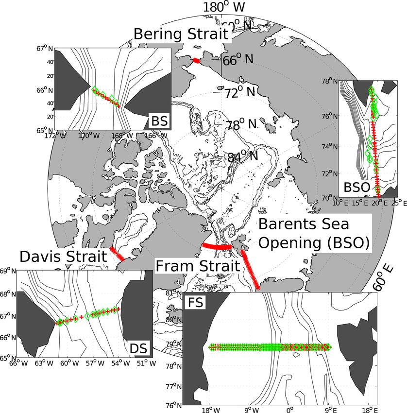
2112                                                                             A. Forryan et al.: Arctic freshwater fluxes

Mann et al., 2017). Arctic freshwater export also has the        ments around the Arctic boundary from summer 2005, apply-
potential to change Atlantic northward heat fluxes through       ing the commonly used box-inverse model technique (Wun-
the disruption of deep convection and consequently, the          sch, 1978) to calculate ocean (including sea ice) volume ex-
strength of the Atlantic meridional overturning circulation      changes between the Arctic and adjacent ocean basins. TB12
(e.g. Manabe and Stouffer, 1995).                                represents a significant advance, resulting in the calculation
   We define a flux of freshwater to mean the rate of addi-      of consistent optimized ocean velocity fields and the first
tion of pure water to (or its removal from) the ocean surface,   quasi-synoptic estimates of Arctic Ocean surface freshwater
by exchanges with the atmosphere (evaporation, E; and pre-       (and heat) fluxes.
cipitation, P ) and by input from the land (runoff, R). The         We here introduce a third method as a modification of the
total ocean surface freshwater flux F is then F = P −E +R.       budget method, which we call the geochemical method, and
There are then three ways to estimate F . The first is to mea-   which requires knowledge of distributions of certain tracers
sure P , E and R each – the “direct” approach of Aagaard and     that describe various sources of ocean waters. These tracers
Carmack (1989); see also Haine et al. (2015), Serreze et al.     can be used to generate source fractions, and we aim to com-
(2006), Dickson et al. (2007) and Carmack et al. (2016). Di-     bine those source fractions with the TB12 velocity field to
rect measurement of Arctic freshwater fluxes is hampered by      calculate new estimates of source fluxes. We next describe
the scarcity of observations (both in situ and remote) and in-   the candidate tracers and their functions.
complete knowledge and understanding of the physical pro-           Bulk ocean waters display a near-constant ratio of oxy-
cesses involving air moisture, clouds, precipitation and evap-   gen isotope concentration, measured as the anomaly from
oration (Vihma et al., 2016; Bring et al., 2016; Lique et al.,   the ocean standard value, δ 18 O (Craig, 1961; Östlund and
2016). This scarcity is compounded by uncertainty in the         Hut, 1984; Redfield and Friedman, 1969). Distillation (iso-
observations themselves (e.g. Aleksandrov et al., 2005) and      topic fractionation) by evaporation and (in the polar oceans)
by sparsely distributed sampling sites (for a full discussion    freezing preferentially removes light isotopes from seawa-
see Vihma et al., 2016). Estimates of runoff are limited by      ter. Evaporated or meteoric water returns to the ocean di-
incomplete river observations (with only ∼ 70 % of Arctic        rectly, as rain- and snowfall, and indirectly, as river runoff
rivers gauged) and understanding of how river discharge is       and (in polar regions) as icebergs and meltwater from terres-
modified in response to permafrost changes and subsurface–       trial ice caps, and these waters have distinctive (low) oxy-
surface water interactions (Bring et al., 2016, 2017). Com-      gen isotope anomalies. In addition, sea ice that has been
pensation for ungauged runoff, arising from incomplete river     frozen out of seawater also has a low δ 18 O; this process
observations, is usually achieved by the use of simple models    leaves behind in the seawater an elevated (positive) δ 18 O
based on linear regression from gauged regions (e.g. Shiklo-     signal. The δ 18 O tracer is conservative, reflecting only the
manov et al., 2000; Lammers et al., 2007). The use of atmo-      net isotopic fractionation that the water sample has under-
spheric reanalysis products (e.g. Haine et al., 2015) to com-    gone. In combination with salinity, it can be used to decom-
pensate for the paucity of direct measurements is in turn ham-   pose water samples into fractions of “seawater” (meaning
pered by the scarcity and uncertainty of observations to con-    bulk ocean water unmodified by local effects of distillation),
strain those reanalyses, which makes accurate modelling of       freshwater of meteoric origin and the ice-modified fraction
all the physical processes involved problematic and leads to     because the end members occupy distinctly separate loca-
relatively unconstrained model dynamics in the Arctic (Lique     tions in δ 18 O–salinity space (Östlund and Hut, 1984). How-
et al., 2016).                                                   ever, unlike salinity, where freshwater has a definite salinity
   The second way to estimate F is what Aagaard and Car-         of zero, there is much variety in the δ 18 O values observed for
mack (1989) call the “indirect” approach, which we call          sea ice, river runoff (Bauch et al., 1995) and glacier ice (Cox
the “budget” approach. The budget approach recognizes that       et al., 2010). Following Östlund and Hut (1984) there have
ocean salinity is sensitive to dilution (or concentration) by    been many studies using δ 18 O to determine fractions of ice
addition (or removal) of freshwater. Therefore with knowl-       melt and meteoric water in the Arctic, most notably in the
edge of fields of velocity and salinity around the boundary      Fram Strait (Dodd et al., 2012; Meredith et al., 2001; Rabe
of a closed volume (to ensure conservation of mass), the sur-    et al., 2013), in the Canada Basin (Yamamoto-Kawai et al.,
face freshwater flux within the volume may be calculated;        2008), and in the East Greenland Current (Cox et al., 2010).
see Serreze et al. (2006), Dickson et al. (2007) and Bacon          Concentrations of dissolved inorganic nutrients in seawa-
et al. (2015). Until recently, Arctic Ocean surface freshwater   ter and the elemental composition of phytoplankton popula-
fluxes had been estimated using heterogeneous and asynop-        tions are observed to occur at broadly the same stoichiomet-
tic compendia of data which, through many years of work,         ric ratios (Redfield et al., 1963). Where nutrient availability
are now beginning to tell a consistent story, though there is    does not limit phytoplankton growth, this indicates that the
still uncertainty in all the major terms (e.g. Serreze et al.,   ratio of the uptake of nutrients (the ratio of nitrate to phos-
2006; Dickson et al., 2007; Haine et al., 2015). The first       phate, in this case) by phytoplankton, known as the Redfield
quasi-synoptic application of the budget approach, by Tsub-      ratio, is fixed. In the Arctic context, this implies that devia-
ouchi et al. (2012, hereafter TB12), used ocean measure-         tions from typical Redfield ratios of seawater concentrations

The Cryosphere, 13, 2111–2131, 2019                                                  www.the-cryosphere.net/13/2111/2019/
A. Forryan et al.: Arctic freshwater fluxes 2113
of these inorganic nutrients may serve as tracers of the ge-
ographic origin of seawaters, which would be useful to un-
derstand seawater pathways through the Arctic Ocean. Fur-
thermore, as a decomposition within seawater, this approach
would generate information orthogonal to that provided by
salinity and δ 18 O.
It is observed that Pacific seawater has higher relative
concentrations of phosphate than Atlantic seawater (Bauch
et al., 1995; Ekwurzel et al., 2001; Jones et al., 1998). Nitrate
concentrations (used in combination with oxygen; Ekwurzel
et al., 2001) are only quasi-conservative, as both are altered
due to biological activity or air–sea exchange in surface wa-
ters (Alkire et al., 2015), while the use of nitrate : phosphate
(N : P) nutrient ratios (Jones et al., 1998) has been considered
to be conservative with respect to biological activity. How-
ever, there is emerging evidence that the N : P ratio may be
becoming non-conservative in the Arctic Ocean as a conse-
quence of sea ice retreat. Denitrification is a process that re-
moves nitrogen from the biogeochemical system, and Bauch
et al. (2011) and Alkire et al. (2019) both note that calcu-
lations based on the N : P ratio overestimate quantities of
Pacific-derived seawaters as a result of denitrification of sea-
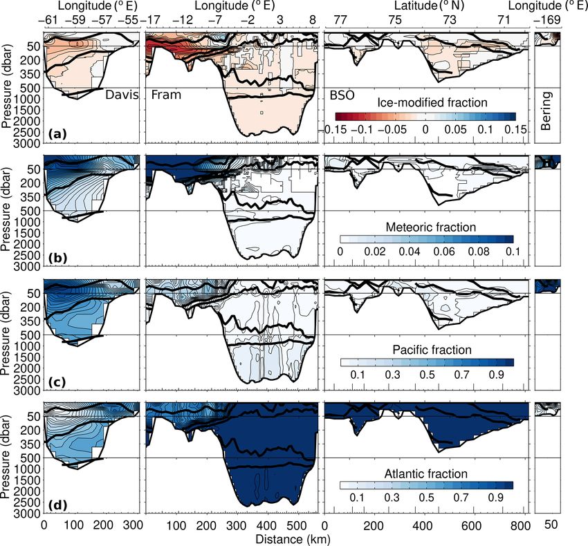
Figure 1. Map of the Arctic Ocean, showing the four main gate-
water in bottom sediments. Also, and despite the N : P ratios ways. The position of the δ 18 O and nutrient sample locations is
for the Atlantic and Pacific oceans exhibiting distinct linear indicated by green diamonds, and the Tsubouchi et al. (2012) CTD
relationships with near-constant slopes, there is variation in station positions by red crosses.
the exact form of this relationship (Jones et al., 2008; Suther-
land et al., 2009; Dodd et al., 2012; Yamamoto-Kawai et al.,
2008). In the Arctic Ocean, nutrient ratios have been used to
trace the circulation of Pacific seawater (Jones et al., 1998; along-boundary horizontal coordinate, which conserves vol-
Jones, 2003), and to indicate the likely origins of freshwa- ume and salinity transports, based on hydrographic data col-
ter sources (Yamamoto-Kawai et al., 2008; Sutherland et al., lected in summer 2005. For further details of the inverse
2009). model construction see TB12. For this study, the TB12 vol-
Our aims in this study are (1) to generate new estimates of ume fluxes are combined with additional tracers to gener-
Arctic Ocean source fluxes using the geochemical approach, ate source component estimates of liquid Arctic freshwater
(2) to compare the results of the established budget approach fluxes, to compare with the existing net (salinity-derived) es-
to those of the new geochemical approach, and (3) to test the timates of TB12.
consistency of the various tracers used. To these ends, we first From the TB12 model, the Arctic boundary circula-
describe the data sources and the model used along with the tion is broadly conventional. Atlantic-origin seawater en-
attribution methods and schemes implemented (Sect. 2). Re- ters through the Barents Sea Opening with a volume flux
sults are presented in Sect. 3, and discussed with an examina- of 3.6 ± 1.1 Sv (± standard deviation). Pacific-origin sea-
tion of the implications for the future use of biogeochemical water enters through Bering Strait with a volume flux of
tracers in the Arctic in Sect. 4. 1.0 ± 0.2 Sv. Fram Strait is a net exporter of seawater, with a
volume flux of 1.6 ± 3.9 Sv, representing a balance between
inflowing (mainly) Atlantic waters in the West Spitsbergen
2 Data and methods Current in the east of the strait (volume flux of 3.8 ± 1.3 Sv)
and outflowing waters in the East Greenland Current in the
2.1 Measurements west of the strait (volume flux of 5.4 ± 2.1 Sv). The net
seawater export through Davis Strait has a volume flux of
TB12 use an inverse model (Wunsch, 1978; Roemmich, 3.1 ± 0.7 Sv. For details of other relatively small contribu-
1980) that considers the Arctic Ocean as a control volume tions to the total, see TB12. As a simplified and approximate
bounded by land and four gateways – Davis, Fram, and summary, ∼ 8 Sv of Atlantic-origin and ∼ 1 Sv of Pacific-
Bering straits and the Barents Sea Opening (Fig. 1) – and origin seawater enters the Arctic, with ∼ 9 Sv of variously
is divided into 15 horizontal layers defined by isopycnal modified seawater exported. The net surface freshwater flux
surfaces. The TB12 inverse model generates an optimized (both liquid and solid) calculated by TB12 is 187 ± 44 mSv,
horizontal velocity field v(s, z), where z is depth and s the 147±42 mSv in the liquid ocean plus 40±14 mSv in sea ice.
www.the-cryosphere.net/13/2111/2019/ The Cryosphere, 13, 2111–2131, 2019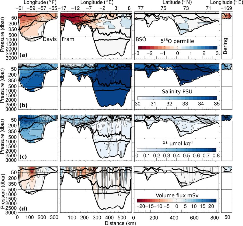
2114                                                                                 A. Forryan et al.: Arctic freshwater fluxes

   Biogeochemical data were originally collated and pub-            cal source water fraction from the Atlantic (and also Pacific)
lished by Torres-Valdés et al. (2013) for inorganic nutrients       Ocean; seawater fractions are always positive. The “mete-
and MacGilchrist et al. (2014) for δ 18 O. Original datasets are    oric” fraction can in principle be either positive, stemming
described as follows. For Davis Strait see Lee et al. (2004)        directly or indirectly from rain- and snowfall, where the in-
(with δ 18 O by Kumiko Azetsu-Scott, Department of Fish-            direct route implies river runoff or terrestrial glacial input to
eries and Oceans, Bedford Institute of Oceanography). For           the ocean, or negative, from evaporation. The “ice-modified”
Bering Strait see Woodgate et al. (2015). For the Barents Sea       fraction is a result of sea ice freezing and melting, and (as
Opening see The International Council for the Exploration           will become apparent) appears mainly in oceanic water as
of the Sea Oceanographic Database (http://www.ices.dk/              negative fractions consequent on the freezing out of sea ice
marine-data/dataset-collections/Pages/default.aspx, last ac-        from oceanic water. For simplicity, therefore, we define this
cess: 13 August 2019) for nutrient data, and Schmidt et al.         (negative) fraction as “brine”, following Östlund and Hut
(1999) for δ 18 O. For Fram Strait see Budéus et al. (2008)         (1984), and use “sea ice meltwater” for the alternative (posi-
and Kattner (2011) for nutrient data, and Rabe et al. (2009)        tive) case. Velocities into (out of) the Arctic Ocean are signed
for δ 18 O. There are no δ 18 O measurements below ∼ 400 m in       positive (negative), so that seawater imports (exports) are
Fram Strait, so we simply extrapolate the deepest measure-          signed positive (negative), imports (exports) of positive frac-
ment to the bottom, for completeness. This depth is close to        tions (rain, snow, rivers, etc.) of meteoric input are signed
the Greenland–Scotland sill depths (600–800 m) to the south,        positive (negative) and brine imports (exports) are signed
so there is little or no net flux below these depths (TB12) and     negative (positive).
we do not expect the absence of deep δ 18 O to significantly           We employ three variants of the approach to the cal-
impact our results. Sample locations are shown in Fig. 1.           culation of the resulting source fractions. Firstly a three-
   Our domain comprises a total of 147 hydrographic sta-            end-member scheme (3EM) is adopted, which uses salin-
tions, which includes data from 16 general circulation model        ity and δ 18 O to identify seawater, meteoric freshwater and
grid cells in the Barents Sea Opening that are used as hy-          ice-modified seawater (mainly brine). Secondly the 3EM
drographic stations, covering a total oceanic distance of           scheme is extended to a four-end-member scheme (4EM)
1803 km, with a total (vertical) section area of 1050 km2 .         through the use of inorganic nutrient data, aiming to discrim-
Vertical resolution is 1 dbar, with maximum pressures of            inate between seawater of Atlantic and Pacific origin, where
1044 dbar in Davis Strait, 2704 dbar in Fram Strait, 471 dbar       the salinity and δ 18 O end-member properties of both ocean
in the Barents Sea Opening, and 52 dbar in Bering Strait (for       sources are assumed to be the same as for Atlantic seawater.
further discussion of the model domain see TB12).                   Thirdly the 4EM scheme is applied again, but now adopting
   The δ 18 O and nutrient data were optimally interpolated         distinct end-member properties for both ocean-source salin-
(Roemmich, 1983) vertically in pressure and horizontally in         ity and δ 18 O (4EM+), replicating previous practice (Dodd
distance to match the TB12 model domain (Fig. 2). The in-           et al., 2012; Jones et al., 2008; Sutherland et al., 2009). The
terpolation recovers the measurements for each sample point         properties of the three schemes are summarized in Table 1.
and interpolates between values to fill the unsampled areas            To discriminate between Atlantic and Pacific seawaters,
of the domain. The resulting nutrient fields show typical fea-      an additional relationship is formulated in terms of the con-
tures, including low concentrations in the upper, sunlit layers     centrations of the inorganic nutrients phosphate and nitrate
as a consequence of nutrient utilization during primary pro-        (Dodd et al., 2012; Jones et al., 1998). We form this rela-
duction, and concentrations that increase with depth due to         tionship in terms of the variable P ∗ , which is an expression
remineralization and/or dissolution of sinking particles; see       describing the excess concentration of phosphate above that
also Torres-Valdés et al. (2013). The δ 18 O sample resolution      which would be expected from typical Redfield nutrient ra-
is mainly adequate to capture the significant Arctic Ocean          tios (Redfield et al., 1963), and it employs the observed ni-
features, although in the Fram Strait section around 6◦ W,          trate concentration
there is only a single station to represent the East Greenland
Current, so that horizontal gradients to either side of this sta-   P ∗ = Pm − (Nm /16),
tion will only be approximate.
                                                                    where Pm and Nm are the measured nitrate and phosphate
                                                                    concentrations respectively. Atlantic and Pacific seawaters
2.2    Approach
                                                                    are each considered to have a distinct, near-constant nitrate-
                                                                    to-phosphate (N : P) ratio (Jones et al., 1998), which can be
Following established practice, the sources of a parcel of
                                                                    expressed algebraically as
oceanic water are considered to number three or four. The
sources are characterized by end members, which are de-             Poce = Pslope Nm + Pint ,
fined points in the phase space populated by the observed
liquid (and solid i.e. sea ice) biogeochemical tracer proper-       where Poce is the estimated concentrations of phosphate from
ties, so that here “oceanic water” means the sum total of all       the relevant ocean (either Atlantic or Pacific) waters and the
liquid fractions. The term seawater is used to mean the typi-       subscripts “slope” and “int” indicates the slope and intercept

The Cryosphere, 13, 2111–2131, 2019                                                     www.the-cryosphere.net/13/2111/2019/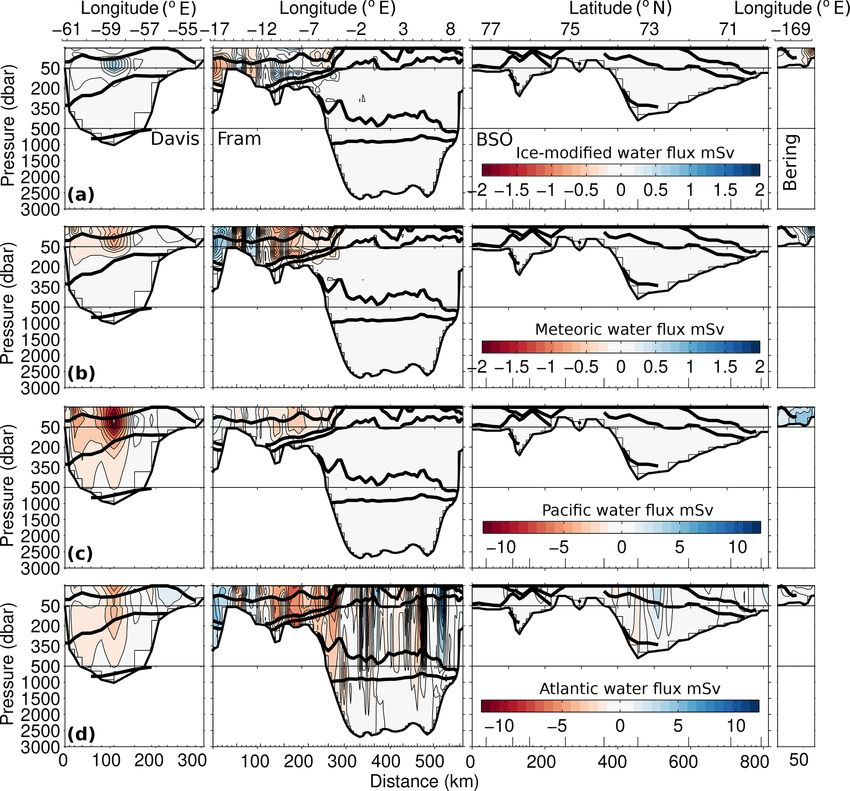
A. Forryan et al.: Arctic freshwater fluxes                                                                                         2115

Figure 2. Sections of δ 18 O (a), salinity (b), P ∗ (c) and volume flux from Tsubouchi et al. (2012) (d) after optimal interpolation onto
the Tsubouchi et al. (2012) CTD station positions, clockwise around the four gateways from Davis Strait to Bering Strait. Solid black
lines indicate the potential density (σ ) surfaces separating the main Arctic water masses grouped as follows: surface water (σ0 < 26.0),
subsurface water (26.0 < σ0 < 27.1), upper Atlantic water (27.1 < σ0 < 27.5), Atlantic water (σ0 = 27.5 to σ0.5 = 30.28), intermediate
water (σ0.5 = 30.28 to σ1 = 32.75) and deep water (σ1 > 32.75); definitions from Tsubouchi et al. (2012). Note the broken scaling of the
y axis.

Table 1. Description of the three model schemes.

                    Schemes     Constraints                Fluxes                        Comments
                    3EM         Volume conservation,       Seawater, meteoric water,     Seawater is assigned a fixed
                                salinity, δ 18 O           ice melt                      salinity regardless of origin.
                    4EM         Volume conservation,       Atlantic seawater, Pacific    Atlantic and Pacific seawa-
                                salinity, δ 18 O, P ∗      seawater, meteoric water,     ters are assigned a common
                                                           ice melt                      salinity and δ 18 O, but dif-
                                                                                         ferent P ∗ values.
                    4EM+        Volume conservation,       Atlantic seawater, Pacific    Atlantic and Pacific seawa-
                                salinity, δ 18 O, P ∗      seawater, meteoric water,     ters have different salinity,
                                                           ice melt                      δ 18 O and P ∗ values.

of the relationships. Boundary sections of salinity, δ 18 O and        water fractions to be determined for each water parcel. Each
P ∗ are shown in Fig. 2.                                               water parcel then has a suite of i = 1, . . ., M measured prop-
   To quantify source fractions for each oceanic water parcel          erties xi . Each measured property is treated as the sum of
(i.e. grid point), we establish the following system of equa-          j = 1, . . ., M fractions fi of a suite of source properties Xi,j .
tions. This problem is conventionally treated as “square”,             The number of source properties (or end members) is M = 3
with the number of constraints equal to the number of source           or 4 here, and the associated freshwater sources are indi-

www.the-cryosphere.net/13/2111/2019/                                                          The Cryosphere, 13, 2111–2131, 2019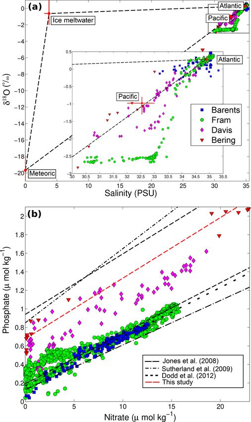
2116                                                                                 A. Forryan et al.: Arctic freshwater fluxes

cated as sea ice (j = 1), meteoric (j = 2), seawater (j = 3
for 3EM), or Pacific and Atlantic seawater (j = 3 and 4 for
4EM variants respectively). Written as a sum,
       M
       X
Xi =          Xi,j fj .
       j =1

Setting all x, X = 1 for i = 1 retrieves the requirement that
the sum of all the source fractions fj accounts for all of the
observed oceanic water:
      M
      X
1=           fj .                                           (1)
      j =1

The measured properties are then δ 18 O concentrations (i =
2) and salinity (i = 3) for all models; in addition the 4EM
variants employ P ∗ for i = 4 (Table 1). The product of this
process is a system of M equations describing M unknowns,
which is written in matrix form for (M × 1) column vectors
f and x, and (M × M) matrix X:

x = Xf .

This is solved for f by standard (exact) inversion of a square
matrix at each water parcel on our ocean boundary grid, to
calculate the resulting spatial distributions of the relevant
oceanic water source fractions:

f = X−1 x.

2.3    End-member values

Previous studies have used different values for the end-
member concentrations of salinity, δ 18 O and nutrients, which
are summarized in Tables 2 and 3. A least-squares linear fit
to the δ 18 O and salinity data from the three sections likely
to contain freshwater of meteoric origin (Davis, Fram and          Figure 3. (a) Salinity–δ 18 O relationship for all samples used in this
Bering straits) suggests a δ 18 O end member in the range of       paper; mean literature end points (± standard deviation) are marked.
−20 ‰ (Bering Strait) to −30 ‰ (Fram Strait), with a mean          Red crosses indicate the mean values of literature end points and
                                                                   black dashed lines the mixing lines between them. (b) Nutrient data
value of −23.3 ‰, which is within the range of the published
                                                                   for all samples used in this paper compared to the published N : P re-
values.
                                                                   lationships of Jones et al. (2008), Dodd et al. (2012) and Sutherland
   The relationships between salinity and δ 18 O for our data      et al. (2009). The dashed red line indicates a best fit to the Bering
and from cited sources are shown in Fig. 3a. This phase            Strait nutrient data presented here. Symbols denoting the data from
diagram is akin to the oceanographer’s “mixing diagram”,           each section are the same in both panels. Note Dodd et al. (2012)
where measured oceanic water properties tend to lie along          uses the same Pacific relationship as Jones et al. (2008).
lines connecting core water mass properties as a result of
mixing between those properties. In this case, processes that
add sea ice meltwater or meteoric water cause mixing along         ice sheet melt, which has a distinctly lighter δ 18 O signature
the lines joining the three end points (seawater, meteoric         (Cox et al., 2010). The fits to data from the three sections
water, sea ice meltwater). The difference here is that there       likely to contain Atlantic seawater (Fram and Davis straits,
are processes that remove water mass constituents (freez-          Barents Sea Opening) suggest an Atlantic seawater salinity
ing, evaporation), and this is manifested on the phase di-         end point of ≈ 35.
agram as points that “back away” from the relevant end                Considering the published nitrate–phosphate relation-
points, clearly seen, for example, in Fig. 3a in the Fram Strait   ships, the most appropriate to this study are the values used
data. The Fram Strait data also exhibit the two-layer mix-         by Jones et al. (2008), Sutherland et al. (2009) and Dodd et al.
ing relationship indicating the likely presence of Greenland       (2012) because Yamamoto-Kawai et al. (2008) include am-

The Cryosphere, 13, 2111–2131, 2019                                                      www.the-cryosphere.net/13/2111/2019/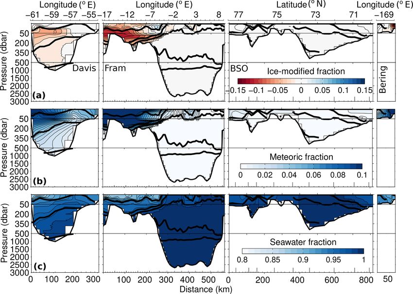
A. Forryan et al.: Arctic freshwater fluxes                                                                                              2117

Table 2. End-member values for salinity and δ 18 O (‰) from the literature. Note Bauch et al. (1995) calculate ice melt δ 18 O by multiplying
measured surface seawater δ 18 O(surf) by a “fractionation factor” of 1.0021.

                                      Atlantic        Pacific            Met.         Melt    Source
                     δ 18 O       0.24 ± 0.03     −0.8 ± 0.1      −20 ± 2         −2 ± 1.0    Yamamoto-Kawai et al. (2008)
                     (‰)                  0.3     −1.0 ± 0.5         −21        1.0021surf    Bauch et al. (1995)
                                          0.3          −1.3        −18.4               0.5    Dodd et al. (2012)
                                  0.19 ± 0.06     −0.8 ± 0.1      −18 ± 2          −2 ± 1     Azetsu-Scott et al. (2012)
                                  0.35 ± 0.15      −1 ± 0.1       −21 ± 2          1 ± 0.5    Sutherland et al. (2009)
                     Mean                0.28          −0.98        −19.7             −0.6
                     Sal.        34.87 ± 0.03     32.5 ± 0.2               0          4±1     Yamamoto-Kawai et al. (2008)
                     (PSU)              34.92             33               0            3     Bauch et al. (1995)
                                         34.9           32.0               0            4     Dodd et al. (2012)
                                 34.75 ± 0.14     32.5 ± 0.2               0          4±1     Azetsu-Scott et al. (2012)
                                    35 ± 0.15       32.7 ± 1               0          4±1     Sutherland et al. (2009)
                     Mean               34.89           32.54              0          3.75

Table 3. P : N relationships, where PO4 = slope × NO3 + intercept               where the integral is taken around the ocean boundary, from
(µmol kg−1 ).                                                                   seabed to surface, and including sea ice; the overbar indicates
                                                                                area mean and prime indicates deviation from the mean, i.e.
                   Slope         Intercept   Source                             S = S 0 +S and v = v 0 +v; and s and z are horizontal and ver-
 Atlantic          0.0545           0.1915   Jones et al. (2008)                tical coordinates respectively. TB12 describe the calculation
                    0.053            0.170   Dodd et al. (2012)                 and method in detail, and they also inspect the assumption
            0.048 ± 0.003     0.130 ± 0.04   Sutherland et al. (2009)           of stationarity, concluding that, for a quasi-synoptic dataset
 Mean              0.052            0.164                                       such as this, it is justified (their Sect. 3.5).
 Pacific           0.0653             0.94   Jones et al. (2008)
                                                                                   Then in the stationary case the surface freshwater flux F
             0.08 ± 0.015      0.85 ± 0.13   Sutherland et al. (2009)           is equal and opposite to the ice and ocean boundary volume
                   0.0654           0.6766   Calculated for this study          transport VO :
                                             from observations
 Mean              0.070            0.822                                       F + VO = 0,

                                                                                where
                                                                                     ‹
monium, and the nutrient measurements used here are of ni-
                                                                                VO =   v(s, z) dsdz.
trate plus nitrite (Torres-Valdés et al., 2013). A least-squares
best fit to the Bering Strait nutrient data has a slope of 0.0654,
which is consistent with that of Jones et al. (2008), and an in-                Lastly, the fraction of the ocean seawater flux per water par-
tercept of 0.6766 (Table 3). The relationships between nitrate                  cel attributed to each n source, δVO , is
and phosphate concentrations for our data and from cited
                                                                                δVO,j (s, z) = fi (s, z)v(s, z)δsδz.
sources are shown in Fig. 3b.

2.4   Freshwater flux calculation                                               2.5   End-member uncertainty

We use the approach established by TB12 and developed by                        Due to the wide range of plausible end-member values for
Bacon et al. (2015), which recognizes that a unique defi-                       each of the water types, to give an estimate of the likely
nition of a freshwater flux is given by the net surface ex-                     uncertainty due to end-member choice, fluxes of the differ-
change between the ocean (including ice) and the adjacent                       ent water types were evaluated using a Monte Carlo tech-
land and atmosphere, i.e. the net of precipitation, evaporation                 nique. Distributions for the different end-member parame-
and runoff. The surface freshwater flux within an enclosed                      ters were constructed from the cited values (Table 2) by
ocean volume is then calculated from its dilution effect on                     assuming the parameter variability is normally distributed,
salinity:                                                                       with mean equal to the mean of the cited values and stan-
                                                                                dard deviation equal to the range. A sample set of 1000
     ‹ 0 0
          vS                                                                    ensembles was drawn from the set of constructed parame-
F=            dsdz,                                                             ter distributions using a Latin hypercube sampling strategy
           S

www.the-cryosphere.net/13/2111/2019/                                                                   The Cryosphere, 13, 2111–2131, 2019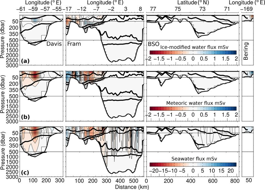
2118 A. Forryan et al.: Arctic freshwater fluxes
fractions were made positive-definite by rounding to zero any
of the fractions that were less than zero, and setting the re-
maining seawater fraction so that Eq. (1) was not invalidated.
3.1 Three-end-member model (3EM)
The distribution of 3EM source fractions is shown in Fig. 5.
Ice-modified waters are found almost exclusively in the sur-
face/upper waters of the model (depths down to 1000 dbar
in the Davis Strait), with the highest-magnitude fractions
(−0.15) found in subsurface waters of the western Fram
Strait between depths of ∼ 50 and 300 dbar. The fractions
of ice-modified waters are mostly negative, indicating brine,
with a small fraction (∼ 0.05) being positive (indicating
fresh meltwater input) in the surface (above 70 dbar) East
Greenland Current (East Greenland Current; between 6.5 and
2◦ W) of the Fram Strait. Meteoric waters are also found al-
most exclusively in the surface/upper waters of the model,
with high fractions (> 0.08) in the surface/subsurface waters
(depths down to 350 dbar) in the Davis Strait and the western
side of the Fram Strait. There is also a high fraction of me-
teoric water in the Bering Strait. Seawater fractions are high
Figure 4. Parameter space for the Monte Carlo simulations. Solid
red line indicates the mean of the published values for the parame- (∼ 1) in all deep and intermediate model waters at depths in
ter; dashed red lines indicate maximum and minimum of published excess of ∼ 350 dbar.
values. Typical volume fluxes (positive indicating into the Arc-
tic) for the 3EM source fractions are shown in Fig. 6. The
strongest fluxes of ice-modified waters occur as brine ex-
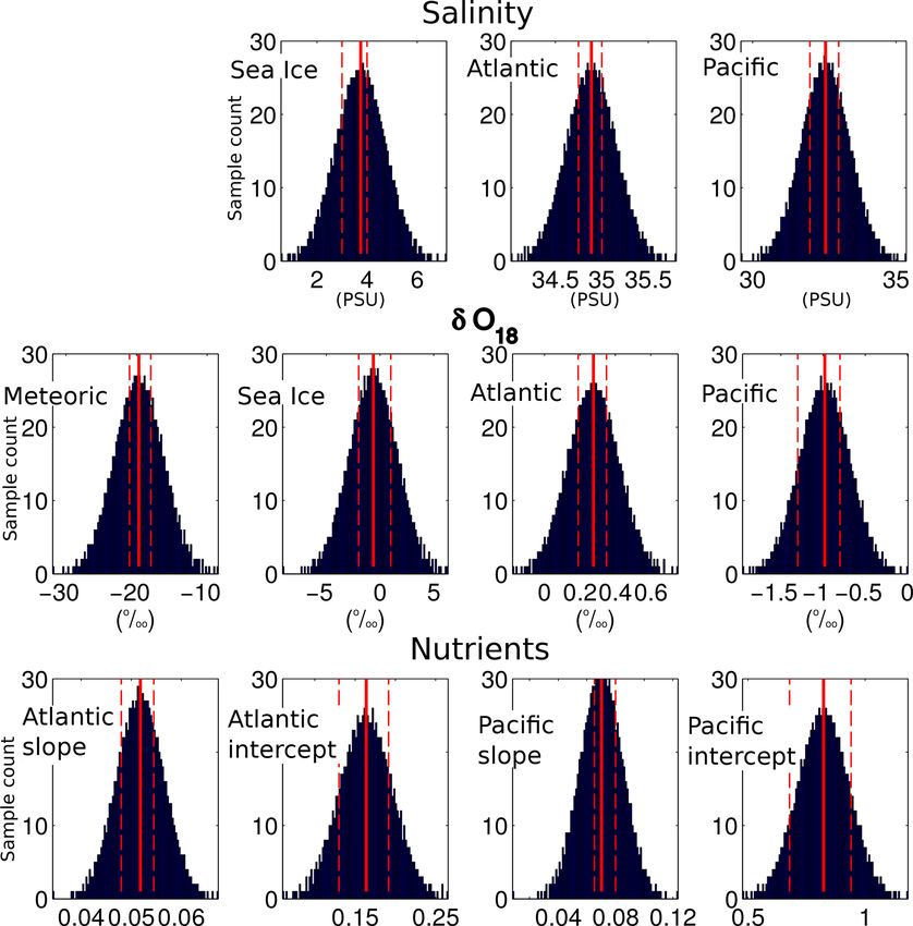
(McKay et al., 1979). The distributions of the individual pa- ports in surface waters of the middle of the Davis Strait and
rameters in the ensemble, which in all cases encompass the on the western side of the Fram Strait (East Greenland Cur-
end points in Sect. 2.3 above, are shown in Fig. 4. Seawater rent), and as brine import to the east in the Bering Strait, with
salinity for 3EM and 4EM models is fixed at the boundary fluxes of ∼ 0.1 Sv in magnitude. The patterns of counter-
area mean salinity for the TB12 model (34.662). A second vailing fluxes over the Belgica Bank (west of 6.5◦ W) in the
choice of seawater salinity end point (35.0) results from the Fram Strait indicate recirculation (see TB12). Meteoric wa-
discussion in Sect. 4. ter volume fluxes follow the same general pattern as for ice-
For each model approach, fluxes of the different water modified waters, with strong export (∼ 0.1 Sv) in the middle
types were estimated by combining the velocities from the of the Davis Strait and the East Greenland Current and strong
TB12 model with the calculated water type fractions for the import (∼ 0.1 Sv) of meteoric waters in the Bering Strait.
sample ensemble. Mean and standard deviations for the at- Seawater volume fluxes resemble the oceanic circulation of
tributed volume fluxes of each water type were calculated as TB12 (as expected), with concentrated exports in Davis Strait
the mean and standard deviation of the results from the sam- (∼ 1 Sv) and the East Greenland Current (∼ 0.5 Sv), and im-
ple ensemble. ports to the east in the Fram Strait in the West Spitsbergen
Current (east of 5◦ E) and in the Bering Strait.
For the 3EM model schemes, the net seawater volume flux
3 Results is effectively zero (0.002 ± 0.006 Sv, Table 4, Monte Carlo
uncertainty quantification). The net volume export of mete-
Here we present the results of the application of the methods oric waters (200 ± 44 mSv) is consistent with the TB12 sur-
and end members, described in Sect. 2, to generate three- face freshwater input of 187 ± 44 mSv (Table 4). The model
and four-end-member freshwater source fractions and fluxes. also indicates a net brine input export (60 ± 50 mSv), which
Equation (1) allows for individual fractions to be either < 0 is similar to the model solid sea ice export of 40 ± 14 mSv,
or > 1 as long as the sum of all fractions is equal to 1. Nega- with the bulk of the brine export occurring through the Davis
tive fractions of meteoric and ice-modified waters result from Strait (Table 4).
removal of freshwater from seawater by evaporation and sea The 3EM model indicates that the volume export of me-
ice formation respectively. However, seawater fractions, ei- teoric water through Fram Strait is concentrated in the Bel-
ther total or individual Atlantic and Pacific water fractions, gica Bank and East Greenland Current regions, 22 ± 6 and
should be positive. Consequently, Pacific and Atlantic water 83 ± 50 mSv respectively, with close to zero meteoric flux in
The Cryosphere, 13, 2111–2131, 2019 www.the-cryosphere.net/13/2111/2019/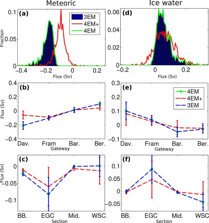
A. Forryan et al.: Arctic freshwater fluxes                                                                                              2119

Figure 5. Sections of ice-modified fraction (a), meteoric fraction (b) and seawater fraction (c), for the 3EM model, clockwise around the
four gateways from Davis Strait to Bering Strait. Solid black lines indicate the isopycnal surfaces separating the main Arctic water masses
as described in Tsubouchi et al. (2012). End members used were the mean of the literature values (see Tables 2 and 3). Note different colour
scales for each panel.

Figure 6. Sections of ice-modified water flux (a), meteoric water flux (b) and seawater flux (c), for the 3EM model (mSv), clockwise around
the four gateways from Davis Strait to Bering Strait. Solid black lines indicate the isopycnal surfaces separating the main Arctic water masses
as described in Tsubouchi et al. (2012). End members used were the mean of the literature values (see Tables 2 and 3). Note different colour
scales for each panel. Positive values indicate flux into the Arctic.

www.the-cryosphere.net/13/2111/2019/                                                             The Cryosphere, 13, 2111–2131, 2019
2120                                                                                 A. Forryan et al.: Arctic freshwater fluxes

Table 4. Mean volume fluxes (Sv ± standard deviation) for the three-end-member (3EM) model. Positive values indicate fluxes into the
Arctic. Values of solid freshwater flux from Tsubouchi et al. (2012).

                                               Oceanic               Met.           Ice melt      Sum
                             Davis      −3.035 ± 0.008    −0.209 ± 0.055      0.100 ± 0.062    −3.144
                             Fram       −1.566 ± 0.004    −0.104 ± 0.027      0.038 ± 0.030    −1.632
                             Barents     3.671 ± 0.004     0.013 ± 0.031     −0.048 ± 0.035     3.636
                             Bering      0.931 ± 0.003     0.099 ± 0.023     −0.029 ± 0.026     1.001
                             Liquid       0.002 ± 0.006   −0.200 ± 0.044      0.060 ± 0.050    −0.139
                             Solid                                           −0.040 ± 0.014     −0.04

Table 5. Mean volume fluxes (Sv ± standard deviation) for the components of the Fram Strait flux (Belgica Bank, BB; East Greenland
Current, EGC; mid-strait, Mid.; West Spitsbergen Current, WSC) from the three-end-member (3EM) model. Positive values indicate fluxes
into the Arctic.

                                               Oceanic               Met.           Ice melt      Sum
                              BB       −0.350 ± 0.001     −0.022 ± 0.006    −0.002 ± 0.006     −0.373
                              EGC      −5.364 ± 0.007     −0.083 ± 0.050     0.088 ± 0.056     −5.359
                              Mid.      0.303 ± 0.000     −0.000 ± 0.003    −0.005 ± 0.003      0.298
                              WSC       3.845 ± 0.004      0.001 ± 0.032    −0.044 ± 0.036      3.803
                              Liquid   −1.566 ± 0.004     −0.104 ± 0.027      0.038 ± 0.030    −1.632

the remainder of the strait (Table 5). This is consistent with       Fram Strait and in the Barents Sea Opening. The distribu-
the picture described in previous studies: Dodd et al. (2012),       tion of meteoric waters in both four-end-member models is
Rabe et al. (2009) and Meredith et al. (2001). Brine is ex-          consistent with the 3EM model where meteoric waters also
ported mainly in the East Greenland Current (88 ± 56 mSv),           mostly occupy the surface layers. However, differences oc-
with small (∼ 5 mSv) fluxes of ice-modified water in the             cur in the Davis Strait, where the 4EM and 4EM+ models
middle and Belgica Bank sections of the strait (Table 5).            indicate lower fractions (∼ 0.01) below ∼ 350 dbar, in the
The apparent brine import in both the West Spitsbergen Cur-          Bering Strait where meteoric water is confined to the eastern
rent and the Barents Sea Opening, 44 ± 36 mSv (Table 4)              side and in the deeper waters of the model where the meteoric
48 ± 35 mSv (Table 5) respectively, reflects the higher δ 18 O       fraction is non-zero (< 0.01). Both four-end-member mod-
values at the surface (∼ 0.4 ‰) relative to those for deeper         els indicate Pacific water mostly in the surface/near-surface
waters (∼ 0.2 ‰)) to the east of 5◦ W (Fig. 2). This is dis-         waters of the Davis, Fram and Bering straits, and almost ex-
cussed in Sect. 4.                                                   clusively Atlantic water in the deepest waters of the model
                                                                     (∼ 0.9). Both models show small fractions of Pacific water
3.2    Four-end-member models (4EM and 4EM+)                         in the deep waters of the Fram Strait and Barents Sea Open-
                                                                     ing (∼ 0.1) and Atlantic water in the Bering Strait (∼ 0.1).
The 4EM scheme extends the 3EM scheme through use of                    Differences between the three- and four-end-member
inorganic nutrient (nitrate and phosphate) data, aiming to dis-      model schemes are also reflected in the fluxes of the differ-
criminate between Atlantic and Pacific seawater origin. The          ent fractions. For both four-end-member models, there are
4EM scheme retains single end points for salinity and δ 18 O,        non-zero fluxes of brine, meteoric water (both < 0.005 Sv)
as in 3EM. In the 4EM+ scheme, distinct salinity and δ 18 O          and Pacific water (< 0.02 Sv) in the deeper waters of the
end-member properties are attributed to Atlantic and Pacific         Fram Strait and Barents Sea Opening. Consistent with the
seawaters, replicating previous practice (Dodd et al., 2012;         3EM model, the 4EM model has a net oceanic volume flux
Jones et al., 2008; Sutherland et al., 2009). The resulting dis-     (sum of Pacific and Atlantic contributions) that is effectively
tributions of 4EM and 4EM+ source fractions are shown in             zero (4EM 0.002 ± 0.006 Sv, Table 6), but the net oceanic
Figs. 7 and 9 respectively, and characteristic volume fluxes         volume flux for the 4EM+ model is non-zero indicating a
for the source fractions in Figs. 8 and 10.                          net export (−0.104 ± 0.051 Sv, Table 8). Net model liquid
   Similar to the 3EM model, both 4EM and 4EM+ mod-                  freshwater export (sum of meteoric and ice-modified frac-
els allocate the bulk of the ice-modified waters, mainly             tions) for the 4EM model is the same as for the 3EM model
brine with some meltwater input, to the surface/upper wa-            (140 ± 67 mSv), while the 4EM+ export is smaller with a
ters. However, both four-end-member schemes indicate small           large relative uncertainty (35 ± 51 mSv).
but non-zero fractions (∼ 0.01) of brine in the east of the

The Cryosphere, 13, 2111–2131, 2019                                                      www.the-cryosphere.net/13/2111/2019/
A. Forryan et al.: Arctic freshwater fluxes 2121
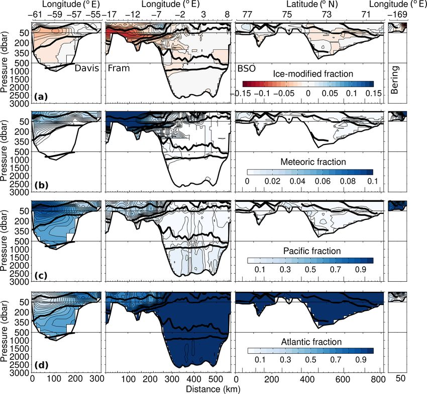
Figure 7. Sections of ice-modified fraction (a), meteoric fraction (b), Pacific fraction (c) and Atlantic fraction (d), for the 4EM model,
clockwise around the four gateways from Davis Strait to Bering Strait. Solid black lines indicate the isopycnal surfaces separating the main
Arctic water masses as described in Tsubouchi et al. (2012). End members used were the mean of the literature values (see Tables 2 and 3).
Note different colour scales for each panel.
Table 6. Mean volume fluxes (Sv ± standard deviation) for the four-end-member (4EM) model. Positive values indicate fluxes into the Arctic.
Values of solid freshwater flux from Tsubouchi et al. (2012).
Atlantic Pacific Met. Ice melt Sum
Davis −0.815 ± 0.346 −2.219 ± 0.346 −0.209 ± 0.055 0.100 ± 0.062 −3.144
Fram −1.333 ± 0.088 −0.233 ± 0.088 −0.104 ± 0.027 0.038 ± 0.030 −1.632
Barents 3.520 ± 0.184 0.151 ± 0.184 0.013 ± 0.031 −0.048 ± 0.035 3.636
Bering 0.126 ± 0.076 0.806 ± 0.076 0.099 ± 0.023 −0.029 ± 0.026 1.001
Liquid 1.497 ± 0.268 −1.495 ± 0.268 −0.200 ± 0.044 0.060 ± 0.050 −0.139
Solid −0.040 ± 0.014 −0.04
The net ice-modified water (mainly brine) flux for both 4EM+ model estimates a smaller net volume flux (98 ±
the 4EM and 4EM+ schemes is also consistent with the 3EM 46 mSv, Tables 6 and 8). Both 4EM and 4EM+ models show
model and the TB12 solid ice flux, with the 4EM model es- the same flux pattern for meteoric water as the 3EM model,
timating 60 ± 50 mSv and the 4EM+ 63 ± 64 mSv (Tables 6 with meteoric water entering the Bering Strait and exiting
and 8). Both 4EM and 4EM+ models show the same flux pat- through the Davis and Fram straits. However, the net import
tern for ice-modified water as the 3EM model, with the bulk of meteoric water through the Bering Strait and the net ex-
of the brine input exiting through the Davis Strait (Tables 4, port of meteoric water through the Davis Strait in the 4EM+
6 and 8, Fig. 11). model schemes is approximately half the magnitude of the
While the net volume flux of meteoric water for the 4EM fluxes in the other two schemes (Tables 4, 6 and 8, Fig. 11).
model is the same as that of the 3EM (200 ± 44 mSv), the
www.the-cryosphere.net/13/2111/2019/ The Cryosphere, 13, 2111–2131, 20192122 A. Forryan et al.: Arctic freshwater fluxes Figure 8. Sections of ice-modified water flux (a), meteoric water flux (b), Pacific water flux (c) and Atlantic water flux (d), for the 4EM model (mSv), clockwise around the four gateways from Davis Strait to Bering Strait. Solid black lines indicate the isopycnal surfaces separating the main Arctic water masses as described in Tsubouchi et al. (2012). End members used were the mean of the literature values (see Tables 2 and 3). Note different colour scales for each panel. Positive values indicate flux into the Arctic. Both 4EM and 4EM+ model schemes indicate an imbal- For the Fram Strait, the pattern of water fluxes described ance in the net volume fluxes for both Pacific and Atlantic by both the 4EM and 4EM+ schemes is consistent with the water. They both show a net export of Pacific water (4EM pattern described above for the 3EM model (Tables 7 and 1.495 ± 0.268 Sv; 4EM+ 1.488 ± 0.263 Sv) that is balanced 9). In both four-end-member schemes, Pacific water is ex- by a net import of Atlantic water of approximately equal ported across Belgica Bank and in the East Greenland Cur- magnitude (4EM 1.497 ± 0.268 Sv; 4EM+ 1.384 ± 0.255 Sv, rent, accounting for approximately 15 % of the Fram Strait Tables 6 and 8). Current understanding of Arctic fluxes sug- oceanic volume flux (Tables 7 and 9). While fluxes of me- gests that Pacific water enters the Bering Strait and exits both teoric and ice-modified waters described by the 4EM model through the Davis Strait, after passing through the western are the same as for the 3EM model (Table 7), the fluxes from Canadian Archipelago, and on the western side of the Fram the 4EM+ schemes are different (Table 9). Strait (Haine et al., 2015). Consistent with this view, both The description of Arctic freshwater fluxes presented by four-end-member schemes indicate that Pacific water, enter- the 4EM+ model is broadly consistent with that from pre- ing the Arctic through the Bering Strait, exits mostly through vious studies of fluxes in the Fram Strait using 4EM+ type the Davis Strait with a much (O(10×)) smaller flux through schemes with distinct Pacific seawater, δ 18 O and salinity end the Fram Strait, mainly across Belgica Bank and in the East members (Dodd et al., 2012; Azetsu-Scott et al., 2012; Rabe Greenland Current. Export of Pacific water through the Davis et al., 2013). Analysis of a time series of observations from Strait is approximately twice the magnitude of the import the Fram Strait suggests a mean freshwater export flux dom- through the Bering Strait (Tables 6 and 8). Atlantic water cir- inated by waters of meteoric origin, mixed with brine to the culates in through the Barents Sea Opening and out through west of 2◦ W in the East Greenland Current and over the the western Fram and Davis straits, with the import through Greenland shelf (Belgica Bank), with fluxes of negative me- the Barents Sea Opening approximately twice the magnitude teoric origin waters also noted in the West Spitsbergen Cur- of the export (Tables 6 and 8). rent (Dodd et al., 2012; Rabe et al., 2013). The Cryosphere, 13, 2111–2131, 2019 www.the-cryosphere.net/13/2111/2019/
A. Forryan et al.: Arctic freshwater fluxes                                                                                           2123

Figure 9. Sections of ice-modified fraction (a), meteoric fraction (b), Pacific fraction (c) and Atlantic fraction (d), for the 4EM+ model,
clockwise around the four gateways from Davis Strait to Bering Strait. Solid black lines indicate the isopycnal surfaces separating the main
Arctic water masses as described in Tsubouchi et al. (2012). End members used were the mean of the literature values (see Tables 2 and 3).
Note different colour scales for each panel.

Table 7. Mean volume fluxes (Sv ± standard deviation) for the components of the Fram Strait flux (Belgica Bank, BB; East Greenland
Current, EGC; mid-strait, Mid.; West Spitsbergen Current, WSC) from the four-end-member (4EM) model. Positive values indicate fluxes
into the Arctic.

                                        Atlantic             Pacific              Met.            Ice melt       Sum
                      BB        −0.182 ± 0.035     −0.167 ± 0.035      −0.022 ± 0.006     −0.002 ± 0.006      −0.373
                      EGC       −4.948 ± 0.376     −0.416 ± 0.377      −0.083 ± 0.050      0.088 ± 0.056      −5.359
                      Mid.       0.226 ± 0.058      0.077 ± 0.058      −0.000 ± 0.003     −0.005 ± 0.003       0.298
                      WSC        3.571 ± 0.274      0.274 ± 0.275       0.001 ± 0.032     −0.044 ± 0.036       3.803
                      Liquid    −1.333 ± 0.088     −0.233 ± 0.088      −0.104 ± 0.027       0.038 ± 0.030     −1.632

   The greatest differences between the models are in the               and 9). Brine export is also lower in the 4EM+ schemes com-
fluxes of meteoric, brine and ice meltwaters across Belgica             pared to the 3EM and 4EM models (Tables 7 and 9; Fig. 11).
Bank and in the East Greenland Current (Fig. 11), with the                 In the Davis Strait the 4EM+ model is qualitatively con-
4EM+ schemes showing less export of meteoric water in the               sistent with previous studies, where source fractions show
East Greenland Current compared to the other schemes. In                the highest freshwater content in the surface waters on the
the 4EM+ model, the import of high-salinity water in the                western side of the strait, from Pacific seawater and meteoric
West Spitsbergen Current is attributed almost equally to neg-           fractions, with a contribution from brine (Azetsu-Scott et al.,
ative meteoric origin water and high-salinity ice-modified              2012). To the east of the Davis Strait, there is a small contri-
(brine input) water, in contrast to the 4EM and 3EM schemes,            bution from sea ice meltwater (Azetsu-Scott et al., 2012).
which attribute this high-salinity import to brine (Tables 7

www.the-cryosphere.net/13/2111/2019/                                                           The Cryosphere, 13, 2111–2131, 2019
2124 A. Forryan et al.: Arctic freshwater fluxes
Figure 10. Sections of ice-modified water flux (a), meteoric water flux (b), Pacific water flux (c) and Atlantic water flux (d), for the 4EM+
model (mSv), clockwise around the four gateways from Davis Strait to Bering Strait. Solid black lines indicate the isopycnal surfaces
separating the main Arctic water masses as described in Tsubouchi et al. (2012). End members used were the mean of the literature values
(see Tables 2 and 3). Note different colour scales for each panel. Positive values indicate flux into the Arctic.
Table 8. Mean volume fluxes (Sv ± standard deviation) for the four-end-member (4EM+) model. Positive values indicate fluxes into the
Arctic. Values of solid freshwater flux from Tsubouchi et al. (2012).
Atlantic Pacific Met. Ice melt Sum
Davis −0.934 ± 0.343 −2.231 ± 0.367 −0.060 ± 0.057 0.080 ± 0.084 −3.144
Fram −1.333 ± 0.079 −0.234 ± 0.086 −0.091 ± 0.025 0.026 ± 0.030 −1.632
Barents 3.493 ± 0.168 0.151 ± 0.185 0.011 ± 0.037 −0.019 ± 0.050 3.636
Bering 0.158 ± 0.089 0.825 ± 0.099 0.041 ± 0.030 −0.023 ± 0.034 1.001
Liquid 1.384 ± 0.255 −1.488 ± 0.263 −0.098 ± 0.046 0.063 ± 0.064 −0.139
Solid −0.040 ± 0.014 −0.04
4 Discussion and summary 4.1 Ice-modified waters
Within uncertainty, the net seawater flux of the 3EM and The models generate apparent brine imports in the West
4EM models is zero: 2 ± 6 mSv for 3EM and 2 ± 379 mSv Spitsbergen Current and the Barents Sea Opening, both with
for 4EM (Tables 4 and 6). Thus in this section, we first dis- magnitude of ∼ 45 mSv and a total of ∼ 90 mSv with a large
cuss the “minority” water mass constituents, meaning ice- relative uncertainty of ∼ 50 mSv. If correct, this is a sub-
modified waters (mainly brine), and Pacific waters and mete- stantial component of the Arctic Ocean freshwater budget.
oric waters, in terms of implications for net fluxes and funda- These (apparent) fluxes are too small to be visible in Fig. 5,
mental points of interpretation; finally, we offer some general but for scale, note that each net (oceanic water) inflow is
perspectives. ∼ 3 Sv, 1 % of which is 30 mSv. These brine fluxes are con-
The Cryosphere, 13, 2111–2131, 2019 www.the-cryosphere.net/13/2111/2019/A. Forryan et al.: Arctic freshwater fluxes 2125
Table 9. Mean volume fluxes (Sv ± standard deviation) for the components of the Fram Strait flux (Belgica Bank, BB; East Greenland
Current, EGC; mid-strait, Mid.; West Spitsbergen Current, WSC) from the four-end-member (4EM+) model. Positive values indicate fluxes
into the Arctic.
Atlantic Pacific Met. Ice melt Sum
BB −0.191 ± 0.034 −0.167 ± 0.035 −0.011 ± 0.005 −0.004 ± 0.007 −0.373
EGC −4.929 ± 0.345 −0.416 ± 0.376 −0.060 ± 0.057 0.046 ± 0.073 −5.359
Mid. 0.231 ± 0.053 0.076 ± 0.056 −0.007 ± 0.004 −0.003 ± 0.005 0.298
WSC 3.556 ± 0.251 0.274 ± 0.273 −0.013 ± 0.040 −0.014 ± 0.051 3.803
Liquid −1.333 ± 0.079 −0.234 ± 0.086 −0.091 ± 0.025 0.026 ± 0.030 −1.632
26, 72) – we find (broadly) salinities and δ 18 O values in the
ranges 35.0–35.2 and 0.2–0.4 ‰ respectively (their Fig. 2).
This combination and range describes the part of the dense
cloud of points heading a short distance north-eastwards in
phase space away from the seawater end point (Fig. 3 panel a
inset).
A consistent interpretation of the apparent West Spitsber-
gen Current and Barents Sea Opening brine imports, there-
fore, is that they are actually manifestations not of local pro-
cesses but rather of source water variability, in the light of our
salinity (34.662) and δ 18 O (mean 0.2 ‰) end points. As a re-
sult, we ran the 3EM model again, now with salinity of 35.0
and fixed δ 18 O of 0.35 ‰; the results are shown in Tables 10
and 11. There is no change to component totals (seawater,
brine, meteoric totals), or to gateway totals (Fram, Davis and
Bering straits, and the Barents Sea Opening), but there are
significant component changes between gateways and within
Fram Strait. For the Barents Sea Opening, we see 38 mSv re-
moved from the seawater component and added to the mete-
oric fraction, approximately doubling the meteoric freshwa-
ter import from 13±31 to 25±7 mSv, more than halving the
ice-modified water flux, which we have been interpreting as
brine import, from 48 ± 35 to 22 ± 7 mSv, and greatly reduc-
Figure 11. Meteoric and ice water volume fluxes. (a, d) Histograms
ing their uncertainties (1 SD), giving us confidence that this
of the total attributed volume fluxes (Sv) for all model schemes.
(b, e) Mean volume fluxes (Sv ± standard deviation) for each gate- new 3EM run is better in this regard. The two freshwater im-
way. (c, f) Volume fluxes (Sv ± standard deviation) for the compo- port values are consistent with freshwater entering the Arc-
nents of the Fram Strait (Belgica Bank, BB; East Greenland Cur- tic Ocean in the Norwegian Coastal Current as the 14 mSv
rent, EGC; mid-strait, Mid.; West Spitsbergen Current, WSC). The of TB12, who use a boundary mean salinity (effective) refer-
3EM model is in blue, the 4EM model in green, and the 4EM+ ence of 34.67, and with the 23 mSv of Smedsrud et al. (2010),
model in red. Positive values indicate fluxes into the Arctic. using a salinity reference of 35.0, as for our new 3EM run re-
spectively. The remaining 22 mSv of ice-modified water is,
therefore, unlikely to be brine import, given the δ 18 O mean
end point of 0.35 ‰; it is more likely to be meltwater ex-
sequences of weakly positive δ 18 O anomalies centred around
port south of Svalbard (see Gammelsrød et al., 2009). A sim-
∼ 300 m depth in both locations, each about 200 m thick and
ilar pattern is seen in the West Spitsbergen Current in the
each spanning ∼ 200 km. The presence of these features in
east of Fram Strait, where an apparent brine import and its
both Fram Strait and the Barents Sea Opening suggests that
uncertainty of 44 ± 36 mSv decrease to 16 ± 4 mSv. For our
they are source water (Atlantic seawater) properties and not
geochemical approach, we began with a salinity end point
the result of modifications by local processes. Frew et al.
that replicated the budget method’s effective salinity refer-
(2000) examine the oxygen isotope composition of north-
ence value; however, we conclude that the geochemical ap-
ern North Atlantic water masses from measurements made
proach requires a different geochemical salinity end point,
in 1991. Considering the waters of interest here – the upper
relevant to the source water properties under consideration.
∼ 500 m in the eastern North Atlantic (their stations 10, 24,
www.the-cryosphere.net/13/2111/2019/ The Cryosphere, 13, 2111–2131, 2019You can also read