Dual-wavelength radar technique development for snow rate estimation: a case study from GCPEx
←
→
Page content transcription
If your browser does not render page correctly, please read the page content below
Atmos. Meas. Tech., 12, 1409–1427, 2019
https://doi.org/10.5194/amt-12-1409-2019
© Author(s) 2019. This work is distributed under
the Creative Commons Attribution 4.0 License.

Dual-wavelength radar technique development for snow rate
estimation: a case study from GCPEx
Gwo-Jong Huang1,2 , Viswanathan N. Bringi2 , Andrew J. Newman3 , Gyuwon Lee1 , Dmitri Moisseev4,5 , and
Branislav M. Notaroš2
1 Center  for Atmospheric REmote sensing (CARE), Kyungpook National University, Daegu 41566, Republic of Korea
2 Department    of Electrical and Computer Engineering, Colorado State University, Fort Collins, Colorado 80523, USA
3 Research Applications Lab, National Center for Atmospheric Research, Boulder, Colorado 80307, USA
4 Institute for Atmospheric and Earth System Research, University of Helsinki, 00560 Helsinki, Finland
5 Finnish Meteorological Institute, 00101 Helsinki, Finland

Correspondence: Gwo-Jong Huang (gwo-jong.huang@colostate.edu)

Received: 29 June 2018 – Discussion started: 6 August 2018
Revised: 13 January 2019 – Accepted: 31 January 2019 – Published: 1 March 2019

Abstract. quantitative precipitation estimation (QPE) of         method by comparing the D3R radar-retrieved SR with ac-
snowfall has generally been expressed in power-law form          cumulated SR directly measured by a well-shielded Pluvio
between equivalent radar reflectivity factor (Ze ) and liquid    gauge for the entire synoptic event.
equivalent snow rate (SR). It is known that there is large
variability in the prefactor of the power law due to changes
in particle size distribution (PSD), density, and fall veloc-
ity, whereas the variability of the exponent is considerably     1   Introduction
smaller. The dual-wavelength radar reflectivity ratio (DWR)
technique can improve SR accuracy by estimating one of the       A detailed understanding of the geometric, microphysical,
PSD parameters (characteristic diameter), thus reducing the      and scattering properties of ice hydrometeors is a vital pre-
variability due to the prefactor. The two frequencies com-       requisite for the development of radar-based quantitative pre-
monly used in dual-wavelength techniques are Ku- and Ka-         cipitation estimation (QPE) algorithms. Recent advances in
bands. The basic idea of DWR is that the snow particle size-     surface and airborne optical imaging instruments and the
to-wavelength ratio is falls in the Rayleigh region at Ku-band   wide proliferation of dual-polarization and multi-wavelength
but in the Mie region at Ka-band.                                radar systems (ground based, airborne or satellite) have al-
   We propose a method for snow rate estimation by using         lowed for observations of the complexity inherent in winter
NASA D3R radar DWR and Ka-band reflectivity observa-             precipitation via dedicated field programs (e.g., Skofronick-
tions collected during a long-duration synoptic snow event on    Jackson et al., 2015; Petäjä et al., 2016). These large field
30–31 January 2012 during the GCPEx (GPM Cold-season             programs are vital given that the retrieval problem is severely
Precipitation Experiment). Since the particle mass can be es-    underconstrained due to large number of geometrical and
timated using 2-D video disdrometer (2DVD) fall speed data       microphysical parameters of natural snowfall, their extreme
and hydrodynamic theory, we simulate the DWR and com-            sensitivity to subtle changes in environmental conditions, and
pare it directly with D3R radar measurements. We also use        co-existence of different populations of particle types within
the 2DVD-based mass to compute the 2DVD-based SR. Us-            the sample volume (e.g., Szyrmer and Zawadzki, 2014).
ing three different mass estimation methods, we arrive at           The surface imaging instruments that give complemen-
three respective sets of Z–SR and SR(Zh , DWR) relation-         tary measurements and are used in a number of recent stud-
ships. We then use these relationships with D3R measure-         ies include (i) 2-D video disdrometer (2DVD; Schönhuber
ments to compute radar-based SR. Finally, we validate our        et al., 2008), (ii) precipitation imaging package (PIP; von
                                                                 Lerber et al., 2017), (iii) Multi-Angle Snowflake Camera

Published by Copernicus Publications on behalf of the European Geosciences Union.
1410                          G.-J. Huang et al.: Dual-wavelength radar technique development for snow rate estimation

(MASC; Garrett et al., 2012). When these instruments are          (Zdr ) in dual-polarization radar technique, where Zdr is used
used in conjunction with a well-shielded GEONOR or PLU-           to estimate Dm (but the physical principles are, of course,
VIO gauge, it is shown that a physically consistent represen-     different; Meneghini and Liao, 2007). The SR is obtained by
tation of the geometric, microphysical, and scattering prop-      “adjusting” the coefficient α in the Ze –SR power law based
erties needed for radar-based QPE can be achieved (Szyrmer        on the estimation of Dm provided by the DWR. The prefactor
and Zawadzki, 2010; Huang et al., 2015; von Lerber et al.,        α depends on the intercept parameter of the PSD (von Lerber
2017; Bukovčić et al., 2018). In this study, we use the 2DVD    et al., 2017) and not on Dm directly. However, because of the
and PLUVIO gauge located within a double fence interna-           apparent negative correlation between Dm and PSD intercept
tional reference (DFIR) wind shield to reduce wind effects.       parameter for a snowfall of a given intensity (Delanoë et al.,
   Radar-based QPE has generally been based on Ze –SR (Ze         2005; Tiira et al., 2016), measurements of Dm can be used to
is reflectivity; SR is liquid equivalent snow rate) power laws    adjust the Ze –SR power law.
of the form Ze = α(SR)β , where the prefactor and expo-              This paper is organized as follows. In Sect. 2, we intro-
nent are estimated based on (i) direct correlation of radar-      duce the approach and methodologies proposed and used in
measured Ze with snow gauges (Rasmussen et al., 2003; Fu-         this study, which may be considered technique development.
jiyoshi et al., 1990; Wolfe and Snider, 2012) or (ii) using       We briefly explain how to estimate the mass of ice particles
imaging disdrometers such as 2DVD or PIP (Huang et al.,           using a set of aerodynamic equations based on Böhm (1989)
2015; von Lerber et al., 2017). Recently, Falconi et al. (2018)   and Heymsfield and Westbrook (2010). We also give a brief
developed Ze –SR power laws at three frequencies (X-, Ka-,        introduction of the scattering model based on particle mass.
and W-band) by direct correlation of radar and PIP observa-       Section 3 provides a brief overview of instruments installed
tions. These studies have highlighted the large variability of    at the test site and the dual-wavelength radar used in this
α due to particle size distribution (PSD), density, fall veloc-   study (D3R: Vega et al., 2014). We analyze surface and D3R
ity, and dominant snow type, whereas the variability in β is      radar data from one synoptic snowfall event during GCPEx
considerably smaller. Similarly, both methods, (i) and (ii),      and compare SR retrieved from DWR-based relations with
have been used to estimate ice water content (IWC) from           SR measured by a snow gauge. The conclusions and possi-
Ze using power laws of the form Ze = a(IWC)b based on             bilities for further improvement of the proposed techniques
airborne particle probe data, direct measurements of IWC,         are discussed in Sect. 4. The acronyms and symbols are listed
and airborne measurements of Ze (principally at X-, Ka-, and      in Appendix.
W-bands) (e.g., Heymsfield et al., 2005, 2016; Hogan et al.,
2006). The advantage of airborne data is that a wide variety
of temperatures and cloud types can be sampled (Heymsfield        2     Methodology
et al., 2016).
   The dual-wavelength reflectivity ratio (DWR, the ratio of      2.1    Estimation of particle mass
reflectivity from two different bands) radar-based QPE was
proposed by Matrosov (1998), Matrosov et al. (2005) to im-        The direct estimation of the mass of an ice particle is difficult
prove SR accuracy by estimating the PSD parameter (me-            and at present there is no instrument available to do this auto-
dian volume diameter D0 ) with relatively low dependence          matically. The conventional method is to use a power-law re-
on density if assumed constant. There has been limited use        lation between the mass and the maximum dimension of the
of dual-λ techniques for snowfall estimation, mainly using        particle of the form m = aD b , where the prefactor a and ex-
vertical-pointing ground radars or nadir-pointing airborne        ponent b are computed via measurements of particle size dis-
radars (Liao et al., 2005, 2008, 2016; Szyrmer and Zawadzki,      tribution N (D) from aircraft probes and independent mea-
2014; Falconi et al., 2018). The dual-λ method is of interest     surements of the total ice water content as an integral con-
to us due to the availability of the NASA D3R scanning radar      straint (Heymsfield and Westbrook, 2010). A similar method
(Vega et al., 2014), which, to the best of our knowledge, has     was used by Brandes et al. (2007), who used 2DVD data for
not been exploited for snow QPE to date.                          N (D) and a snow gage for the liquid equivalent snow ac-
   The DWR is defined as the ratio of the equivalent radar re-    cumulation over periods of 5 min. These methods are more
flectivity factors at two different frequency bands. The main     representative of an average relation when one particle type
principle in DWR is that the particle’s size-to-wavelength ra-    (e.g., snow aggregates) dominates the snowfall with large de-
tio falls in the Rayleigh region at a low-frequency band (e.g.,   viations possible for individual events with differing particle
Ku-band) but in the Mie region at a high-frequency band           types (e.g., graupel).
(e.g., Ka-band) (Matrosov, 1998; Matrosov et al., 2005; Liao         To overcome these difficulties a more general method
et al., 2016). Previous studies have shown that the DWR can       was proposed by Böhm (1989) based on estimating mass
be used to estimate Dm , where Dm is defined as the ratio of      from fall velocity measurements, geometry, and environmen-
the fourth moment to the third moment of the PSD expressed        tal data if the measured fall velocity is in fact the terminal ve-
in terms of liquid-equivalent size or mass (Liao et al., 2016).   locity (i.e., in the absence of vertical air motion or turbulence
In this sense the DWR is similar to differential reflectivity     and in more or less uniform precipitation). The methodol-

Atmos. Meas. Tech., 12, 1409–1427, 2019                                              www.atmos-meas-tech.net/12/1409/2019/
G.-J. Huang et al.: Dual-wavelength radar technique development for snow rate estimation                                        1411

ogy has been described in detail by Szyrmer and Zawadzki            eras (referred to as cameras A and B) which can capture the
(2010), Huang et al. (2015), and von Lerber et al. (2017), and      particle image projection in two orthogonal planes (two side
we refer to these articles for details. The essential feature       views). As mentioned earlier the area ratio (Ar ) should be
is the unique nonlinear relation between the Davies (1945)          obtained from the projected image in the plane normal to
number (X) and the Reynolds number (Re), where X is the             the flow (i.e., top or bottom view). However, to the best of
ratio of mass to area or m/A0.25r   (Ar = Ae /A is the area ra-     our knowledge, there are no ground-based instruments that
tio, where Ae is the effective projected area normal to the         can automatically and continuously capture the horizontal
flow and A is the area of the minimum circumscribing cir-           projected views (i.e., in the plane orthogonal to the flow)
cle or ellipse that completely contains Ae ) and the Re is the      of precipitation particles (however, 3-D-reconstruction based
product of terminal fall speed and the characteristic dimen-        on multiple views can give this information; Kleinkort et al.,
sion of the particle. We have neglected the environmental pa-       2017). Compared with other optical-based instruments, such
rameters (air density, viscosity) as well as boundary layer         as HVSD (hydrometeor velocity size detector; Barthazy et
depth of Abraham (1970) and the inviscid drag coefficient.          al., 2004) or SVI (snow video imager; Newman et al., 2009),
The procedure is to (i) compute Re from fall velocity mea-          which only captures the projected view in one plane, the
surements and characteristic dimension of the particle (usu-        2DVD offers views in two orthogonal planes, giving more
ally the maximum dimension), (ii) compute the Davies num-           geometric information. Figure 1 shows a snowflake observed
ber X, which is expressed as a nonlinear function of Re, and        by a 2DVD from two cameras. The thick black line is the
boundary layer parameters (C0 = 0.6 and δ0 = 5.83; Böhm,            contour of the particle and the thin black lines show the holes
1989) and (iii) estimate particle mass from X and Ar . Heyms-       inside the particle. The effective projected area Ae in the defi-
field and Westbrook (2010) proposed a simple adjustment             nition of area ratio is easy to compute by counting total pixels
(based on field and tank experiments) by defining a mod-            from the particle’s image, and then multiplying by horizon-
ified Davies number as proportional to m/A0.5  r    along with      tal and vertical pixel width. The blue line is the minimum
different boundary layer constants (C0 = 0.292; δ0 = 9.06)          circumscribed ellipse. The area of the ellipse is A in the def-
from Böhm. Their adjustment was shown to be in very good            inition of area ratio. The size of particle measured by 2DVD
agreement with recent tank experiments by Westbrook and             is called the apparent diameter (Dapp ) which is defined as the
Sephton (2017), especially for particles like pristine den-         diameter of the equivalent volume sphere (Schönhuber et al.,
drites with low Ar and at low Re. Note that the difference          2000; Huang et al., 2015). The Dapp is used when comput-
of C0 and δ0 in Böhm and Heymsfield–Westbrook equations             ing Re, as mentioned earlier. The area ratio and Dapp are the
is mainly due to differences in the shape-correcting factor         geometric parameters that are used in our implementation of
(Ar ) to find the optimal relation between drag coefficient (or     the Böhm method.
Davies number, X) and Reynolds number (Re). This is the                In our application of the HW method, the A is based on the
main parameterization error in this set of equations.               diameter of the circumscribed circle that completely encloses
                                                                    the projected pixel area (Ae ), which is easy to calculate from
2.2   Geometric and fall speed measurements                         the contours in Fig. 1. Thus the area ratio is Ae /A, while
                                                                    the characteristic dimension in Re is the diameter of the cir-
One source of uncertainty in applying the Böhm or Heyms-            cumscribing circle. Note that the area ratio and characteristic
field and Westbrook (HW) method is calculating the area             dimension in Re depend on the type of instrument used (e.g.,
ratio (Ar ) using instruments such as 2DVD or precipitation         advanced version of snow video imager by von Lerber et al.,
instrument package (PIP) as they do not give the projected          2017; the HVSD by Szyrmer and Zawadzki, 2010). These
area normal to the flow (i.e., they do not give the needed top      instruments give a projected view in one plane only and thus
view, but rather the 2DVD gives two side views on orthogo-          geometric corrections are used as detailed in the two refer-
nal planes as illustrated in Fig. 1). This is reasonable for snow   ences.
aggregates which are expected to be randomly oriented. The             The two optic planes of the 2DVD are separated by around
other source of uncertainty is in the definition of characteris-    6 mm and the accurate distance is based on calibration by
tic dimension used in Re, which in the HW method is taken to        dropping 10 mm steel balls at three corners of the sensing
be the diameter of the circumscribing circle that completely        area (details of the calibration as well as accuracy of size, fall
encloses the projected area, the maximum dimension (Dmax ;          speed, and other geometric measures are given in Bernauer
this is what we use for the 2DVD in our application of the          et al., 2015). During certain time periods, more than one pre-
HW method). For the Böhm method we use the procedure in             cipitation particle falls in the 2DVD observation area. Since
Huang et al. (2015), which used Dapp defined as the equal-          the two cameras look in different directions, the particles ob-
volume spherical diameter.                                          served by camera A and camera B need to be paired. This
   The two-dimensional video disdrometer (2DVD) used                pairing procedure is called “matching”, and it is illustrated in
herein is described in Schönhuber et al. (2000), and calibra-       Fig. 2. The time period [t1 , t2 ] is dependent on the assumed
tion and accuracy of the instrument are detailed in Bernauer        reasonable fall speed range. Assuming that the minimum and
et al. (2015). The 2DVD is equipped with two line-scan cam-         maximum reasonable fall speeds are vmin and vmax , respec-

www.atmos-meas-tech.net/12/1409/2019/                                                 Atmos. Meas. Tech., 12, 1409–1427, 2019
1412 G.-J. Huang et al.: Dual-wavelength radar technique development for snow rate estimation
Figure 1. A snowflake observed by a 2DVD from two views. The thick black line is the contour of the snowflake and the thin black lines
show the holes inside the snowflake. The effective area, Ae , equals the area enclosed by the thick black curve minus the area enclosed by
thin lines. The blue line represents the minimum circumscribed ellipse, the enclosed area of which is denoted by A.
tively, the distance between two optic planes is Dd , and cam-
era A observed a particle at t0 , we have t1 = t0 + Dd /vmax
and t2 = t0 + Dd /vmin . After matching, the fall speed can be
calculated as Dd /1t, where 1t is the time difference be-
tween two cameras observing the same particle. Because the
fall speed of the 2DVD is dependent on matching, the ge-
ometric features and fall speeds will be in error when mis-
match occurs. Huang et al. (2010) analyzed snow data from
the 2DVD and found that the 2DVD manufacturer’s match-
ing algorithm for snow resulted in a significant mismatching
problem (see also Bernauer et al., 2015). In the Appendix
of Huang et al. (2010), they showed that the mismatch will
cause the volume, vertical dimension, and fall speed of par-
Figure 2. Illustration of the matching procedure. In the situation
ticles to be overestimated. Subsequently, the mass of parti-
shown, it is assumed that camera A observed a particle at time t0 ,
cles will also be overestimated, mainly because of fall speed. and afterwards during a certain time period, t1 to t2 , camera B ob-
To get the best estimation of mass, they used 2DVD single- served two particles. The matching procedure decides which par-
camera data and re-did the matching based on a weighted ticle observed by camera B is the same particle observed by cam-
Hanesch criteria (Hanesch, 1999). If the match criteria are era A.
not satisfied, then that particle is rejected; it follows that the
concentration will tend to be underestimated. To readjust the
measured concentration for this underestimate (assumed to ter of the circumscribing circle or ellipse cannot be obtained
be a constant factor), the procedure described in Huang et without contour data. The only quantity included in single-
al. (2015) is used, which only involves the ratio of the to- camera data is Ae in terms of number of pixels. The Huang
tal number of particles counted in the scan area of the single and Bringi approach (Huang et al., 2015) is referred to as HB,
camera to the number of successfully matched particles in the because both PSD (particle size distribution) and reflectivity
virtual measurement area. For the event analyzed here (using (Ze ) are computed using Dapp as the measure of particle size.
method 1 in Sect. 3.3), this adjustment factor is between 1.1 For methods 2 and 3 in Sect. 3.3, we used the manufac-
and 1.5. The Pluvio gauge accumulation is not used as a con- turer’s matching algorithm, which gives the contour data. To
straint in method 1. The disadvantage of using single-camera avoid overestimating mass due to mismatch, we need to filter
data, as described in Huang et al. (2015), is that the particle out those particles with unreasonable fall speeds. The ver-
contour data are not available (i.e., the manufacturer’s code tical dimension of the particle’s image before match is ex-
does not provide line scan data from single camera). With- pressed as a number of scan lines (i.e., how many scan lines
out contour data, both Dapp and A can only be estimated by are masked by the particle). After match (so vt is known), the
the maximum width of the scan line and height of the parti- vertical pixel width is vt /fs , where fs is the scan frequency
cle as detailed in Huang et al. (2015). Moreover, the diame- of a camera (∼ 55 kHz), and the vertical size of the particle
Atmos. Meas. Tech., 12, 1409–1427, 2019 www.atmos-meas-tech.net/12/1409/2019/G.-J. Huang et al.: Dual-wavelength radar technique development for snow rate estimation 1413
Table 1. Hanesch 2DVD scan line criteria.
Max of total Difference of
scan lines scan lines
≤ 201414 G.-J. Huang et al.: Dual-wavelength radar technique development for snow rate estimation
model at W-band and concluded that the axis ratio can be
used as a tuning parameter. They also showed the impor-
tance of size integration to compute Ze , i.e., the product of
N(D) and the radar cross section for the soft spheroid vs.
complex-shape aggregates. Their result implied that smaller
particles had a larger value for the product when using a soft
spheroid of 0.6 axis ratio relative to complex aggregates and
vice versa for larger particles, leading to compensation when
Ze is computed by size integration over all sizes. Thus, the
soft spheroid model with axis ratio at 0.8 used by Huang et
al. (2015), and which is used herein at Ku- and Ka-bands, is
a reasonable approximation.
The second scattering model we used herein is from Liao
et al. (2013), who use an effective fixed density approach to
justify the oblate spheroid model. To compare the scattering
properties of a snow aggregate with its simplified equal-mass
spheroid, Liao et al. (2013) used six-branch bullet rosette
snow crystals with maximum dimensions of 200 and 400 µm
as two basic elements that simulate snow aggregation. They
computed the backscattering coefficient, extinction coeffi- Figure 4. A map of the GCPEx field campaign. The five test sites
cient, and asymmetry factor for simulated snowflakes, using are CARE, Sky Dive, Steam Show, Bob Morton, and Huronia. The
the DDA and for the corresponding spheres and spheroids ground observation instruments, namely 2DVD, D3R, and Pluvio,
with the same mass but density fixed at 0.2 or 0.3 g cm−3 , and used in this research, were located at CARE.
hence the apparent sphere volume equals the mass divided by
the assumed fixed density. They showed that, when the fre-
quency was lower than 35 GHz (Ka-band), the Mie scattering sites were located north of Toronto, Canada between Lake
properties of spheres with a fixed density equal to 0.2 g cm−3 Huron and Lake Ontario. The GCPEx had five test sites,
were in a good agreement with the scattering results for the namely CARE (Centre for Atmospheric Research Experi-
simulated complex-shaped aggregate model with the same ments), Sky Dive, Steam Show, Bob Morton, and Huronia.
mass using the DDA (see also Kuo et al., 2016). They also The locations of five sites are shown in Fig. 4. The CARE
showed this agreement with a spheroid model with a fixed site was the main test site for the experiment, located at
axis ratio of 0.6 and random orientation. Here, we use the 44◦ 130 58.4400 N, 79◦ 460 53.2800 W and equipped with an ex-
Liao et al. (2013) equivalent spheroid model with a fixed tensive suite of ground instruments. The 2DVD (SN37) and
effective density of 0.2 g cm−3 at Ku- and Ka-bands (note OTT Pluvio2 400 used for observations and analyses in this
that we estimate the mass of each particle from 2DVD mea- paper were installed inside a DFIR (double fence intercom-
surements as described in Sect. 2.1). Note that this fixed- parison reference) wind shield. The dual-frequency dual-
density spheroid scattering model is not based on micro- polarized doppler radar (D3R) was also located at the CARE
physics (where the density would fall off inversely with in- site (Vega et al., 2014) near the 2DVD. The instruments used
creasing size) but on scattering equivalence with a simulated in this paper are depicted in Fig. 5. Because the radar and
(same-mass) complex-shaped aggregate snowflake (Liao et the instrumented site were nearly collocated, we can effec-
al., 2016). tively view the set-up as similar to a vertical-pointing radar
as described in more detail in Sect. 3.2.
We examine a snowfall event on 30–31 January 2012
3 Case analysis that occurred across the GCPEx study area between roughly
22:00 UTC, 30 January and 04:00 UTC, 31 January. Details
3.1 Test site instrumentation and the synoptic event of this case using King City radar and aircraft spiral de-
scent over the CARE site is given in Skofronick-Jackson
The GPM Cold-season Precipitation Experiment (GCPEx) et al. (2015). This event resulted in liquid accumulations of
was conducted by the National Aeronautics and Space roughly 1–4 mm across the GCPEx domain with fairly uni-
Administration (NASA), USA, in cooperation with Envi- form snowfall rates throughout the event. At the CARE site
ronment Canada in Ontario, Canada from 17 January to the accumulations over an 8 h period were < 3.5 mm. Echo
29 February 2012. The goal of GCPEx was “. . . to char- tops as measured by high-altitude airborne radar were 7–
acterize the ability of multi-frequency active and passive 8 km. The precipitation was driven by a shortwave trough
microwave sensors to detect and estimate falling snow. . . ” moving from southwest to northeast across the domain. Fig-
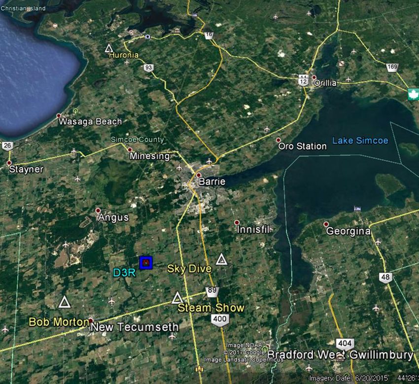
(Skofronick-Jackson et al., 2015). The field experiment ure 6 displays the 850 hPa geopotential heights (m), tem-
Atmos. Meas. Tech., 12, 1409–1427, 2019 www.atmos-meas-tech.net/12/1409/2019/G.-J. Huang et al.: Dual-wavelength radar technique development for snow rate estimation 1415
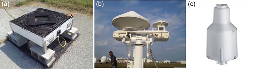
Figure 5. Instruments used in this study: (a) 2DVD (SN37), (b) D3R (dual-wavelength dual-polarized doppler radar), and (c) OTT
Pluvio2 400 precipitation gauge.
perature (K), relative humidity (%), and winds (m s−1 ) at
00:00 UTC, 31 January, during the middle of the accumu-
lating snowfall. A trough axis is apparent just to the west of
the GCPEx domain (green star in Fig. 6). Low-level warm-
air advection forcing upward motion is coincident with high
relative humidity on the leading edge of the trough, over
the GCPEx domain (Fig. 6). Temperatures in this layer were
around −10 to −15 ◦ C throughout the event, supporting effi-
cient crystal growth, aggregation, and potentially less dense
snowfall as this is in the dendritic crystal temperature zone
(e.g., Magono and Lee, 1966). Aircraft probe data during a
descent over the CARE site between 23:15 and 23:43 UTC
showed the median volume diameter (D0 ) of 3 mm, with
particles up to a maximum of 8 mm (aggregates of den-
drites) at 2.2 km m.s.l. with a large concentration of smaller
sizes < 0.5 mm (dendritic and irregular shapes; Skofronick-
Jackson et al., 2015). At the surface, photographs of the pre-
cipitation types by the University of Manitoba showed small Figure 6. The 00:00 UTC, 31 January 2012, 850 hPa geopotential
irregular particles and aggregates (< 3 mm) at 23:30 UTC on heights (m, black solid contours), temperature (K, red: above freez-
30 January. ing, blue: below freezing), relative humidity (%, green shaded con-
tours), and wind (m s−1 , wind barbs). The red dot in the center right
3.2 D3R radar data portion of the figure denotes the general location of the GCPEx field
instruments.
The D3R is a Ku- and Ka-band dual-wavelength polarimet-
ric scanning radar. It was designed for ground validation of
rain and falling snow from GPM satellite-borne DPR (dual-
frequency precipitation radar). The two frequencies used in
the D3R are 13.91 GHz (Ku) and 35.56 GHz (Ka). These two of detecting “meteo” vs. “nonmeteo” echoes) being the tex-
frequencies were used for scattering computations in this re- ture of the standard deviation (SD) of the differential propa-
search as well. Some parameters of the D3R radar relevant gation phase (ϕdp ). We randomly selected 20 out of 85 RHI
for this paper are shown in Table 2. The range resolution of sweeps from 31 January 2012 and computed the SD of Ku-
the radar is adjustable but usually set to 150 m and the near- band ϕdp for each beam over 10 consecutive gates where
field distance is ∼ 300 m; the practical minimum operational SNR ≥ 10 dB. According to the histogram of the SD of ϕdp ,
range is around 450 m. The minimum detectable signal of 90 % of the values were less than around 8◦ . Radar data at
the D3R is −10 dBZ at 15 km. This means that when Zh is a range gate m are identified as “good” data (i.e., meteoro-
−10 dBZ at 15 km, the signal-to-noise ratio (SNR) is 0 dB. logical echoes) only if the standard deviation of ϕdp from
Therefore, the SNR at any range, r, can be computed as fol- the (m − 5)th gate to the (m + 4)th gate is less than 8◦ . This
lows: criterion sets a good data mask for each beam at Ku-band.
15 On the other hand, the ϕdp at Ka-band was determined to be
SNR (r) = Zh (r) + 10 + 20log10 [dB]. (1) too noisy and hence not used herein. The good data mask
r for the Ka-band beam is set by the mask determined by the
The SNR is a very important indicator for radar data quality Ku-band criteria, with the additional requirement that the Ka-
control (QC), the other important parameter for QC (in terms band SNR > 3 dB for the range gate to be considered good.
www.atmos-meas-tech.net/12/1409/2019/ Atmos. Meas. Tech., 12, 1409–1427, 20191416 G.-J. Huang et al.: Dual-wavelength radar technique development for snow rate estimation
Table 2. Some D3R parameters relevant for this study. Full D3R
specifications can be found in Vega et al. (2014).
Ku Ka
Frequency (GHz) 13.91 35.56
Min detectable signal −10 dBZ at 15 km
Range (km) 0.45–30
Range resolution (m) 150
Anterior beam width ∼ 1◦
Note that both radars are mounted on a common pedestal so
that the Ku and Ka-band beams are perfectly aligned.
There are four scan types that can be performed by
the D3R, namely PPI (plan position indicator), RHI (range
height indicator), surveillance, and vertical pointing. Figure 7
shows the scan strategies of the D3R on 31 January 2012, Figure 7. D3R scan strategies on 31 January 2012. The y axis is
azimuth angle (RHI; red x) or elevation angle (PPI; blue o). The
which consisted of a fast PPI scan (surveillance scan; 10◦ per
scan rate of RHI was 1◦ s−1 and 10◦ s−1 for PPI.
second) followed by four RHI scans (1◦ per second), except
from 01:00 to 02:00 UTC. The RHI scans with an azimuth
angle of 139.9◦ point to the Steam Show site and those at
87.8◦ point to the Sky Dive site. There were no RHI scans
pointing to the Bob Morton site, and Huronia (52 km) was
beyond the operational range (maximum 30 km) of the D3R.
During the most intense snowfall the D3R scans did not cover
the instrument clusters at the Sky Dive and Steam Show sites.
So we were left with the analysis of the D3R radar data at
close proximity to the 2DVD or effectively vertical-pointing
equivalent using RHI data from 75 to 90◦ at the nearest prac-
tical range of 600 m. PPI scan data at low elevation angle (3◦ )
were also used from range gate at 600 m. The assumption
is that there is little evolution of particle microphysics from
about 600 m height to the surface and that the synoptic-scale
snowfall was uniform in azimuth (confirmed by Skofronick-
Jackson et al., 2015). The snowfall was spatially uniform
around the CARE site so we selected data at 600 m range
to be compared with the 2DVD and Pluvio observations (this Figure 8. The time series of averaged raw Zh at the CARE site.
range was selected based on the minimum operational range There are two problems indicated in this figure: (i) the Ku-band Zh
of 450 m; see Table 2) to which 150 m was added based on is smaller than the Ka-band Zh on average. (ii) Compared with the
close examination of data quality. For RHI scans, the Zh at Ka-band, there are many too small values of the Ku-band Zh .
each band was averaged over the beams from 75 to 90◦ . The
75◦ is obtained from 600·cos(75◦ ) ≈ 155 m which is close to
the range resolution. For the fast PPI scan, Zh was averaged evation angle is smaller than 78◦ , the unreasonably low Zh
over all azimuthal beams at 600 m range. disappears. Therefore, the RHI scans with azimuth angles
Figure 8 shows the time profile of the averaged Ze at Ku- larger than 300◦ were averaged over the 75 to 78◦ elevation
and Ka-bands. There are two problems indicated in this fig- angles. To compute the DWR, we need to know the Z off-
ure. First, theoretically, the Ku-band Ze should be greater set between the two bands. The measured Zh includes three
than or equal to the Ka-band Ze . The smaller Ku-band Zh components (neglecting attenuation):
indicates that a Z offset exists at both bands. The other prob-
lem is that, compared with the Ka-band, there are many dips Zhmeas = Zhtrue ± error (Zh ) + Zoffset , (2)
in the Ku-band Zh . By comparing Fig. 8 with Fig. 7, we
found that these dips occur only at RHI scans with azimuth where “error” refers to measurement fluctuations (typically
angle larger than 300◦ . We examined those RHI scans beam with standard deviation of ∼ 1 dB). The DWR is obtained as
by beam from 90 to 75◦ . We further found that when the el- the difference between Ku-band Zh and Ka-band Zh , with Zh
Atmos. Meas. Tech., 12, 1409–1427, 2019 www.atmos-meas-tech.net/12/1409/2019/G.-J. Huang et al.: Dual-wavelength radar technique development for snow rate estimation 1417
al. (2015) as well as 1 min averaged N (Dapp ) is calcu-
lated. Note that the scattering model is based on the soft
spheroid model with fixed axis ratio = 0.8 and appar-
ent density ρ. The results obtained by this method are
denoted HB in the figures and in the rest of the paper.
2. Use the manufacturer’s (Joanneum Research, Graz,
Austria) matching algorithm and filter-mismatched
snowflakes as described in Sect. 2.2. The mass is com-
puted from Böhm’s equations. The PSD adjustment fac-
tor is based on using the Pluvio gauge accumulation
as a constraint. Following Liao et al. (2013) as far as
the scattering model is concerned, the density is fixed
at 0.2 g cc−1 and the volume is computed from mass =
density · volume. The effective equal-volume diameter
is Deff and the corresponding PSD is denoted N (Deff ),
which is different from N (Dapp ) in (1) above. Hence-
Figure 9. The averaged raw Zh for Ku- and Ka-bands. The Zh was forth, this method is denoted LM.
randomly selected from 20 of 85 RHI scans with Ku-band Zh <
0 dBZ, range < 1 km, and Ka-band SNR > 3 dB. 3. Use Joanneum matching and filtering method as in (2)
but compute mass using Heymsfield–Westbrook equa-
tions as well as the revised Deff and N (Deff ). This
being in units of dBZ. The measured DWR is as follows: method is denoted HW. Thus, the only difference with
(2) is in the estimation of mass and the difference in Deff
DWRmeas = DWRtrue ∓ error (DWR) + 1Zoffset , (3) and N (Deff ). The PSD adjustment factor is based on us-
ing the Pluvio gauge accumulation as a constraint. The
where error (DWR) is now increased, since the Ku- and Ka- scattering model follows Liao et al. (2013).
band measurement fluctuations are uncorrelated (standard
deviation of around 1.4 dB). The 1Zoffset is determined by The 2DVD measured liquid equivalent snow rate (SR) can be
selecting data where the scatterers (snow particles) are suffi- computed directly from mass as follows:
ciently small in size so that Rayleigh scattering is satisfied at N X M
both bands, i.e., DWRtrue = 0 dB. The criteria are used here 3600 X Vj h i
SR = ; mm h−1 , (4)
to select gates where Ku-band Zh < 0 dBZ along with spa- 1t i=1 j =1 Aj
tial averaging, which reduces the measurement fluctuations
in DWR to estimate 1Zoffset in Eq. (3). Figure 9 shows the where 1t is the integral time (typically 60 s), N is the number
averaged Zh for the two bands from 20 RHI scans which sat- of size bins (typically 101 for the 2DVD), M is the number
isfy the conditions above. After removing three extreme val- of snowflakes in the ith size bin, and Aj is the measured area
ues (outliers) from Fig. 9, 1Zoffset was estimated as −1.5 dB, of the j th snowflake. Further, Vj is the liquid equivalent vol-
which is used in the subsequent data processing. ume of the j th snowflake, so it is directly related to the mass.
Figure 10 compares the liquid equivalent accumulation com-
3.3 2DVD data analysis puted using the three methods above based on 2DVD mea-
surements with the accumulation directly measured by the
The 2DVD used in this study was also located at the CARE collocated Pluvio snow gauge. The Pluvio-based accumula-
site. The particle-by-particle mass estimation is based on tion at the end of the event (03:30 Z) was 1.9 mm while the
three methods as follows: 2DVD-measured accumulations using the three methods are
1.27 mm (HB), 1.45 mm (LM), and 1.24 mm (HW). It is ex-
1. Following the procedure in Huang et al. (2015) we pected that the PSDs of LM and HW should be underesti-
use 2DVD single-camera data and apply the weighted mated because of eliminating mismatched particles which,
Hanesch-matching algorithm (Hanesch, 1999) to re- in principle, could be rematched. Rematching mismatched
match snowflakes. A PSD adjustment factor is com- particles is a research topic on its own and is beyond the
puted as in Huang et al. (2015) without using the Plu- scope of this paper. We used a simple way to adjust the PSD
vio gauge as a constraint. Mass is computed from fall for methods 2 and 3 by scaling the PSD by a constant so
speed, Dapp and environmental conditions using Böhm that the final accumulation matches the Pluvio gauge accu-
(1989). The apparent density of the snow (ρ) is defined mulation. Specifically, the PSD adjustment factors are 1.3
3 . A mean power-law relation of the form
as 6m/π Dapp for LM and 1.52 for HW. Note that PSD adjustment of HB
β
ρ = αDapp is derived for the entire event as in Huang et (method 1) is not done by forcing 2DVD accumulation to
www.atmos-meas-tech.net/12/1409/2019/ Atmos. Meas. Tech., 12, 1409–1427, 20191418 G.-J. Huang et al.: Dual-wavelength radar technique development for snow rate estimation
Figure 10. Comparison of liquid equivalent accumulations com-
puted using HB, LM, and HW methods based on 2DVD measure-
ments and that were directly measured by the collocated Pluvio
snow gauge. We used the total accumulation to estimate the PSD
adjustment factor for the LM and HW methods.
agree with Pluvio, rather the method described in Huang et
al. (2015) is used giving the adjustment factor of 1.54 for
00:00–00:45 UTC and 1.11 for 00:45–04:00 UTC. From the
Pluvio accumulation data in Fig. 10 the SR is nearly constant
at 0.7 mm h−1 between relative times of 1.5 and 3 h (or actual
time from 01:00 on 30 January to 02:30 UTC).
The radar reflectivities at the two bands are simulated by
using the T-matrix method assuming a spheroid shape with
an axis ratio of 0.8, consistently with Falconi et al. (2018).
The PSD is adjusted for methods 1, 2, and 3 as described
above. The orientation angle distribution is assumed to be
quasi-random with Gaussian distribution for the zenith angle Figure 11. Comparison of the 2DVD-derived Zh with D3R mea-
[mean = 0◦ , σ = 45◦ ] and uniform distribution for the az- surements for the entire event, Ku-band (a), and Ka-band (b). This
imuth angle. However, other studies have assumed σ = 10◦ synoptic system started at around 21:00 Z on 30 January and ended
(Falconi et al., 2018). The recent observations of snowflake at around 03:30 Z on 31 January 2012. Ze by LM is close to HW
orientation by Garrett et al. (2015) indicate that substantial and slightly higher, whereas the HB method gives the lowest Ze .
Ze results computed by all methods generally agree with D3R mea-
broadening of the snow orientation distribution can occur due
sured Zh .
to turbulence. Figure 11 compares the time series of D3R-
measured Zh with the 2DVD-derived Ze for the entire event
(20:00–03:30 UTC at (a) Ku- and (b) Ka-band). The Ze for
both bands computed by the three methods generally agree From 00:45 to 01:30 UTC on 31 January 2012, the three
with the D3R measurements to within 3–4 dB. Overall, LM 2DVD-derived Ze simulations deviate systematically from
gives the highest Ze and HB gives the lowest, which is espe- the D3R results for both bands. The other period is from
cially evident at Ka-band. This is consistent with scattering 23:00 to 23:30 UTC on 30 January 2012, when the Ku-band
calculations by Kuo et al. (2016) of single spherical snow Ze has significant deviation from the D3R observations but
aggregates using constant density (0.3 g cc−1 ) giving higher the Ka-band Ze generally agrees with the D3R. Note that
radar cross sections and size-dependent density, i.e., density this synoptic event started at around 21:00 UTC on 30 Jan-
falls off as inverse size (giving lower cross sections). This uary and stopped at 03:30 UTC. We checked the D3R data
feature is consistent with the scattering models referred to and found that, before 22:30 UTC, the RHI scans were from
herein as LM and HB. 0 to 60◦ , so there were no usable data available for com-
parison with the 2DVD and Pluvio at the CARE site. We
note that at 00:30 UTC the King City C-band radar recorded
Atmos. Meas. Tech., 12, 1409–1427, 2019 www.atmos-meas-tech.net/12/1409/2019/G.-J. Huang et al.: Dual-wavelength radar technique development for snow rate estimation 1419
Zh in the range 15–20 dBZ around the CARE site, which
is in reasonable agreement with the D3R radar observations
(Skofronick-Jackson et al., 2015).
Figure 12a compares the time series of DWR simu-
lated from 2DVD observations with the D3R measurements,
whereas Fig. 12b shows the scatterplot In general, HB ap-
pears in qualitatively better agreement (better correlated and
with significantly less bias) with D3R measurements rela-
tive to both LM and HW (significant underestimation rel-
ative to D3R). The scatterplot in Fig. 12b is an important
result since in the HB method the soft spheroid scattering
model is used with density varying approximately inverse
with Dapp (density-Dapp power law where the larger snow
particles have lower density). Hence for a given mass the
Dapp is larger (relative to Ka-band wavelength) and enters
the Mie regime, which lowers the radar cross section at Ka-
band (relative to same mass but constant density radar cross
section in LM and HW). Whereas at Ku-band the differ-
ence in radar cross sections is less between the two methods
(Rayleigh regime). The significant DWR bias in LM and HW
relative to DWR observations is somewhat puzzling in that
the Liao et al. (2013) scattering model radar cross sections
agree with the synthetic complex shaped snow aggregates
of the same mass at Ka-band, whereas the HB model un-
derestimates the radar cross section relative to the synthetic
complex shaped aggregates. On the other hand, Falconi et
al. (2018) demonstrate that the soft spheroid model is ade-
quate at X (close to Ku-band) and Ka-band and by inference
adequate for DWR calculations with the caveat that different
effective axis ratios may need to be used at Ka- and W-bands.
We also refer to airborne (Ku, Ka) band radar data at
00:30 UTC which showed DWR measurements of 3–6 dB
about 1 km height MSL around the CARE site but nearly
0 dB above that all the way to the echo top (Skofronick-
Figure 12. Comparison of the 2DVD-derived DWR using HB, LM,
Jackson et al., 2015). The latter is not consistent with aircraft
and HW methods with the D3R-measured DWR. Panel (a) shows
spirals over the CARE site about an hour earlier where max-
the time profile of the D3R, and (b) shows the scatterplot.
imum snow sizes reach ∼ 8 mm. In spite of the difficulty in
reconciling the observations from the different sensors, the
appropriate scattering model in this particular event appears More case studies are clearly needed to understand the appli-
to favor the soft spheroid model used in HB based on better cability of the LM and HW methods of simulating DWR.
agreement with DWR observations. The other factor to be
considered is the PSD adjustment factor, which is assumed 3.4 Snow rate estimation
constant and independent of size, which may not be the case,
especially for the LM and HW methods as considerable filter- To obtain radar–SR relationships, we use the 2DVD data and
ing is involved due to mismatch (as discussed in Sect. 2.2). simulations. Since we employ a constant PSD adjustment
Note that a constant PSD adjustment factor will not affect factor, it will scale both Ze and SR similarly. Figure 13 shows
DWR but it will affect Ze . For the HB method Huang et the scatterplot of the 2DVD-derived Ze vs. 2DVD-measured
al. (2015) determined the PSD adjustment factor for four SR along with a power-law fit as Z = aSRb . The fitting
events by comparing the 2DVD PSD to that measured by a method used is based on weighted total least square (WTLS)
collocated SVI (snow video imager which was assumed to so the power law can be inverted without any change. The
be the “truth”) for each size bin. The PSD adjustment was coefficients and exponents of the power-law Z–SR relation-
found to not be size dependent for the HB method. On the ship for both bands and three methods are given in Table 3.
other hand, because of the filtering of mismatched particles It is obvious from Fig. 13 that there is considerable scatter
by the LM and HW methods, the PSD adjustment factor may at Ku-band for all three methods with the normalized stan-
be size dependent in which case the DWR will also change. dard deviation (NSD), ranging from 55 % to 70 %. Whereas
www.atmos-meas-tech.net/12/1409/2019/ Atmos. Meas. Tech., 12, 1409–1427, 20191420 G.-J. Huang et al.: Dual-wavelength radar technique development for snow rate estimation
Table 3. Coefficients and exponents of the power-law Z–SR rela-
tionship for HB, LM, and HW methods and Ku- and Ka-bands, re-
spectively.
Method Band a b SD (mm h−1 ) NSD (%)
Ku 140.52 1.48 0.2156 70.99
HB
Ka 60.17 1.18 0.1366 44.97
Ku 129.27 1.64 0.2235 55.89
LM
Ka 99.85 1.25 0.1614 40.35
Ku 106.25 1.58 0.1889 55.30
HW
Ka 66.96 1.42 0.1473 43.11
at Ka-band the scatter is significantly lower with NSD from
40 % to 45 %. The errors in Table 3 are generally termed pa-
rameterization errors.
By using dual-wavelength radar, we can estimate SR using
Ze at two bands as follows:
b0
(
SRKu = a10 · ZKu1
b0 , (5)
SRKa = a20 · ZKa2
0
where a 0 = (1/a)b and b0 = 1/b. To reduce error, we may
take the geometric mean of these two estimators as follows:
SR = (SRKu · SRKa )1/2 = c · ZKu
d
· DWRe , (6)
where c = (a10 a20 )1/2 , d = (b10 + b20 )/2, and e = −b20 /2. Note
that the DWR in Eq. (6) is on a linear scale, i.e., expressed as
a ratio of reflectivity in units of mm6 m−3 . Using Table 3 to
set the initial guess of (c, d, e), nonlinear least squares fitting
was used to determine the optimized (c, d, e) with the cost
function being the squared difference between the 2DVD-
based measurements of SR and cZKu d DWRe , where Z
Ku and
DWR are from 2DVD simulations. Figure 14 shows the SR
computed from the 2DVD simulations of Ku-band Ze and the
DWR using Eq. (6) vs. the 2DVD-measured SR. The (c, d, e)
values for the three methods are given in Table 4. As can also
be seen from Fig. 14 and Table 4, the SR(ZKu , DWR) using
the LM method results in the lowest NSD of 28.49 %, but the
other two methods have similar values of NSD (≈ 30 %) and,
as such, these differences are not statistically significant. Al-
though SR(ZKu , DWR) has a smaller parameterization error
than Ze –SR, the SR(ZKu , DWR) estimation is biased high
when SR < 0.2 mm h−1 (see Fig. 14). When SR is small,
the size of snowflakes is usually also small and falls in the
Rayleigh region at both frequencies, resulting in DWR very
close to 1 (when expressed as a ratio). This implies that there
is no information content in the DWR so including it just
adds to the measurement error. Hence, for small SR or when
DWR ≈ 1, we use the Ze –SR power law.
So far the single-frequency SR retrieval algorithms were Figure 13. 2DVD-derived Zh vs. 2DVD-measured SR scatterplots,
based on 2DVD-based simulations with a PSD adjustment with Z–SR power-law fits, for Ku- and Ka-bands and the HB
factor using the total accumulation from Pluvio as a con- method (a), LM method (b), and HW method (c).
straint. The algorithm we propose for radar-based estimation
Atmos. Meas. Tech., 12, 1409–1427, 2019 www.atmos-meas-tech.net/12/1409/2019/G.-J. Huang et al.: Dual-wavelength radar technique development for snow rate estimation 1421
Table 4. Coefficients and exponents of the SR(ZKu ,DWR) relation
(see Eq. 10) for three methods.
Method c d e SD NSD
(mm h−1 ) (%)
HB 0.0632 0.6537 −0.9155 0.0986 32.45
LM 0.0995 0.5648 −1.3415 0.1139 28.49
HW 0.1017 0.5426 −1.1772 0.1076 31.52
of SR is to use Eq. (6) when DWR > 1 and SR > 0.2 mm h−1 ,
else we use the ZKa –SR power law (note that we do not use
the ZKu -SR power law as the measurement errors of ZKu
seem to be on the high side, Fig. 9). The precise thresholds
used herein are ad hoc and may need to be optimized using
a much larger data set. Figure 15a shows the radar-derived
accumulation using ZKa –SR vs. the Pluvio accumulation vs.
time. The total accumulation from the Pluvio is 2.5 mm and
the three radar-based total accumulations, for HB, LM, and
HW methods amount to [2.6, 1.8, 2.6 mm]. Except for the
underestimation in the LM method (−28 %), the other two
methods agree with the Pluvio accumulation in this event.
Figure 15b is the same as Fig. 15a, except the combination
algorithm mentioned above is used. For this case, ∼ 33 % of
data used the ZKa –SR power law due to threshold constraints
given above. The event accumulations for HB, LM, and HW
methods amount to [2.4, 1.9, 2.2 mm], which are consistent
with the algorithm that uses only the ZKa –SR power law.
However, the criteria of relative bias error in the total ac-
cumulation (in events with low accumulations such as this
one) are not necessarily an indication that the DWR-based
algorithm is not adding value. Rather, the criteria should be
snow rate intercomparison, which could not be done due to
the low resolution (0.01 mm min−1 ) of the Pluvio2 400 gauge
along with the low event total accumulation of only 2.5 mm.
A close qualitative examination of Fig. 15b shows that the
HB method more closely “follows” the gauge accumulation
relative to HB in time in Fig. 15a. In Fig. 15, the time grid
is different for the radar-based data and the gauge data. It is
common to linearly interpolate the gauge data to the radar
sampling time and if this is done, the rms error for the HB
method reduces from 0.1 mm (when using only the ZKa –SR
power law) to 0.045 mm for the DWR algorithm, which con-
stitutes a significant reduction by a factor of 2.
The total error in the radar estimate of SR is composed
of both parameterization errors as well as measurement er-
rors with measurement errors dominating, since the DWR in-
volves the ratio of two uncorrelated variables. From Sect. 8.3
of Bringi and Chandrasekar (2001), the total error of SR in
Eq. (6) is around 50 % (ratio of standard deviation to the
mean). The assumptions are (a) the standard deviation of the
Figure 14. Estimated SR using Ze and DWR of the 2DVD and
measurement of Ze is 0.8 dB, (b) the standard deviation of the
Eq. (10) vs. 2DVD SR scatterplot for the HB method (a), LM
method (b), and HW method (c). DWR (in dB) measurement is 1.13 dB, and (c) the parameter-
ization error is 30 % from Table 4. However, considering the
www.atmos-meas-tech.net/12/1409/2019/ Atmos. Meas. Tech., 12, 1409–1427, 20191422 G.-J. Huang et al.: Dual-wavelength radar technique development for snow rate estimation
and snow gage measurements are unbiased based on accu-
rate calibration. A more elaborate approach of quantifying
uncertainty in precipitation rates is described by Kirstetter et
al. (2015).
4 Summary and conclusions
The main objective of this paper is to develop a technique for
snow estimation using scanning dual-wavelength radar oper-
ating at Ku- and Ka-bands (D3R radar operated by NASA).
We use the 2-D video disdrometer and collocated Pluvio
gauge to derive an algorithm to retrieve snow rate from re-
flectivity measurements at the two frequencies compared to
the conventional single-frequency Ze –SR power laws. The
important microphysical information needed is provided by
the 2DVD to estimate the mass of each particle knowing the
fall speed, apparent volume, area ratio, and environmental
factors from which an average density-size relation is de-
rived (e.g., Huang et al., 2015; von Lerber et al., 2017; Böhm,
1989; Heymsfield and Westbrook, 2010).
We describe in detail the data processing of 2DVD cam-
era images (in two orthogonal planes) and the role of par-
ticle mismatches that give erroneous fall speeds. We use
the Huang et al. (2015) method of rematching using single-
camera data but also use the manufacturer’s matching code
with substantial filtering of the mismatched particles since
the apparent volume and diameter (Dapp ) are more accurate.
To account for the filtering of the mismatched particles, the
particle size distribution (in methods 2 and 3 in Sect. 3.3)
is adjusted by a constant factor using the total accumulation
from the Pluvio as a constraint.
Two scattering models are used to compute the ZKu and
ZKa , termed the soft spheroid model (Huang et al., 2015;
Figure 15. Comparison of the radar-derived accumulated SR us-
HB method) and the Liao–Meneghini (LM) model, which
ing HB, LM, and HW methods with Pluvio gauge measurement.
(a) The radar SR is computed by ZKa –SR relationships. The Pluvio- uses the concept of effective density. In these two methods
accumulated SR on 03:18 UTC is 2.48 mm. The radar-accumulated the particle mass is based on Böhm (1989). The method of
SRs for HB, LM, and HW are 2.64, 1.81, and 2.66 mm. (b) The Heymsfield and Westbrook (2010) is also used to estimate
radar SR is computed by combining SR(ZKu ,DWR) and ZKa –SR mass which is similar to Böhm (1989) but is expected to be
as described in the text. The accumulated SR derived from the radar more accurate (Westbrook and Sephton, 2017); along with
using HB method is 2.38 mm, using LM it is 1.94 mm and using the LM model for scattering, this method is termed HW.
HW it is 2.24 mm. The case study chosen is a large-scale synoptic snow event
that occurred over the instrumented site of CARE during
GCPEx. The ZKu and ZKa were simulated based on 2DVD
Ze fluctuations in Fig. 9, the measurement standard deviation data and the three methods, i.e., HB, LM, and HW yielded
probably exceeds 0.8 dB, especially at Ku-band. Thus, suffi- similar values within ±3 dB. When compared with D3R
cient smoothing of DWR is needed to minimize the measure- radar measurements extracted as a time series over the in-
ment error as much as possible while maintaining sufficient strumented site, the LM and HW methods were closer to
spatial resolution. the radar measurements with the HB method being lower by
Note that the error model used here is additive with the ≈ 3 dB. Some systematic deviations of simulated reflectivi-
parameterization, and measurement errors modeled as zero ties by the three methods from the radar measurements were
mean and uncorrelated with the corresponding error vari- explained by a possible size dependence of the PSD adjust-
ances estimated either from data or via simulations (as de- ment factor.
scribed in Sect. 7 of Bringi and Chandrasekar, 2001). This The direct comparison of DWR (ratio of ZKu to ZKa ) from
is a simplified error model since it assumes that radar Z simulations with DWR measured by radar showed that the
Atmos. Meas. Tech., 12, 1409–1427, 2019 www.atmos-meas-tech.net/12/1409/2019/G.-J. Huang et al.: Dual-wavelength radar technique development for snow rate estimation 1423 HB method gave the lowest bias with the data points more The snow rate estimation algorithms developed here are or less evenly distributed along the 1 : 1 line. The simulation expected to be applicable to similar synoptic-forced snow- of DWR by LM and HW methods underestimated the radar fall under similar environmental conditions (e.g., tempera- measurements of DWR quite substantially, even though the ture and relative humidity) but not, for example, to lake effect correlation appeared to be reasonable. The reason for this dis- snowfall as the microphysics are quite different. However, crepancy is difficult to explain since a constant PSD adjust- analyses of more events are needed before any firm conclu- ment factor (different for method 1 relative to methods 2 and sions can be drawn as to applicability to other regions or en- 3 in Sect. 3.3) would not affect the DWR. From the scatter- vironmental conditions. ing model viewpoint, the LM method takes into account the complex shapes of snow aggregates via an effective density approach, whereas the HB method uses soft spheroid model Data availability. The data used in this study can be made available with density varying approximately inversely with size. We upon request to the corresponding author. did not attempt to classify the particle types in this study. The retrieval of SR was formulated as SR = c·ZKu d ·DWRe , where [c, d, e] were obtained via nonlinear least squares for the three methods. The total accumulation from the three methods using radar-measured ZKu and DWR were com- pared with the total accumulation from the Pluvio (2.5 mm) to demonstrate closure. The closest to Pluvio was the HB method (2.4 mm), next was the HW method (2.24 mm) and then there was LM (1.94 mm). At such low total accumu- lations, the three methods show good agreement with each other as well as with the Pluvio gauge. The poor resolution of the gauge combined with the relatively low total accu- mulation in this event precluded direct comparison of snow rates. The combined estimate of parameterization and mea- surement errors for snow rate estimation was around 50 %. From variance decomposition, the measurement error vari- ance as a fraction of the total error variance was 58 %, and the parameterization error variance fraction was 42 %. Further, the DWR was responsible for 90 % of the measurement error variance, which is not surprising since it is the ratio of two uncorrelated reflectivities. Thus, the DWR radar data have to be smoothed spatially (in range and azimuth) to reduce this error, which will degrade the spatial resolution but is not ex- pected to pose a problem in large-scale synoptic snow events. www.atmos-meas-tech.net/12/1409/2019/ Atmos. Meas. Tech., 12, 1409–1427, 2019
You can also read