Multiscale fractal dimension analysis of a reduced order model of coupled ocean-atmosphere dynamics
←
→
Page content transcription
If your browser does not render page correctly, please read the page content below
Research article
Earth Syst. Dynam., 12, 837–855, 2021
https://doi.org/10.5194/esd-12-837-2021
© Author(s) 2021. This work is distributed under
the Creative Commons Attribution 4.0 License.

        Multiscale fractal dimension analysis of a reduced order
            model of coupled ocean–atmosphere dynamics
                            Tommaso Alberti1 , Reik V. Donner2,3 , and Stéphane Vannitsem4
                             1 INAF-IAPS, via del Fosso del Cavaliere 100, 00133 Rome, Italy
          2 Department of Water, Environment, Construction and Safety, Magdeburg–Stendal University of Applied
                                  Sciences, Breitscheidstraße 2, 39114 Magdeburg, Germany
           3 Research Department IV – Complexity Science and Research Department I – Earth System Analysis,

                 Potsdam Institute for Climate Impact Research (PIK) – Member of the Leibniz Association,
                                       Telegrafenberg A31, 14473 Potsdam, Germany
                               4 Royal Meteorological Institute of Belgium, Brussels, Belgium

                              Correspondence: Tommaso Alberti (tommaso.alberti@inaf.it)

                               Received: 30 December 2020 – Discussion started: 13 January 2021
                            Revised: 21 June 2021 – Accepted: 5 July 2021 – Published: 6 August 2021

      Abstract. Atmosphere and ocean dynamics display many complex features and are characterized by a wide
      variety of processes and couplings across different timescales. Here we demonstrate the application of multi-
      variate empirical mode decomposition (MEMD) to investigate the multivariate and multiscale properties of a
      reduced order model of the ocean–atmosphere coupled dynamics. MEMD provides a decomposition of the orig-
      inal multivariate time series into a series of oscillating patterns with time-dependent amplitude and phase by
      exploiting the local features of the data and without any a priori assumptions on the decomposition basis. More-
      over, each oscillating pattern, usually named multivariate intrinsic mode function (MIMF), represents a local
      source of information that can be used to explore the behavior of fractal features at different scales by defining
      a sort of multiscale and multivariate generalized fractal dimensions. With these two complementary approaches,
      we show that the ocean–atmosphere dynamics presents a rich variety of features, with different multifractal
      properties for the ocean and the atmosphere at different timescales. For weak ocean–atmosphere coupling, the
      resulting dimensions of the two model components are very different, while for strong coupling for which cou-
      pled modes develop, the scaling properties are more similar especially at longer timescales. The latter result
      reflects the presence of a coherent coupled dynamics. Finally, we also compare our model results with those
      obtained from reanalysis data demonstrating that the latter exhibit a similar qualitative behavior in terms of mul-
      tiscale dimensions and the existence of a scale dependency of the statistics of the phase-space density of points
      for different regions, which is related to the different drivers and processes occurring at different timescales in
      the coupled atmosphere–ocean system. Our approach can therefore be used to diagnose the strength of coupling
      in real applications.

1   Introduction                                                  while the North Atlantic Oscillation (NAO) affects extrat-
                                                                  ropical northern hemispheric regions at seasonal and decadal
The atmosphere and the ocean form a complex system whose          timescales (Ambaum et al., 2001). The sources of these pro-
dynamical variability extends over a wide range of spatial        cesses have been widely investigated by means of multi-
and temporal scales (Liu, 2012; Xue et al., 2020). As an          ple data analysis methods and various types of modeling
example, the tropical regions are markedly characterized by       (e.g., Philander, 1990; Czaja and Frankignoul, 2002; Van der
inter-/multi-annual processes like the El Niño–Southern Os-       Avoird et al., 2002; Mosedale et al., 2006; Kravtsov et al.,
cillation (ENSO) (Neelin et al., 1994; Meehl et al., 2003),

Published by Copernicus Publications on behalf of the European Geosciences Union.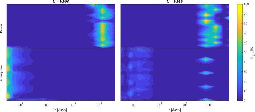
838                                      T. Alberti et al.: Multivariate analysis of a reduced order ocean–atmosphere model

2007; Feliks et al., 2011; Liu, 2012; L’Hévéder et al., 2014;
Farneti, 2017; Vannitsem and Ghil, 2017; Wang, 2019; Xue                            PM(`)
                                                                                           pk log pk
                                                                     .                 k=1
et al., 2020, and references therein), highlighting how the at-   D1 = lim lim                       ,                          (2)
                                                                         `→0N→∞           log `
mospheric low-frequency variability (LFV) is related to the
ocean. The latter develops thanks to the interaction with the     and the correlation dimension
ocean mixed layer (OML) driven by a mixing process due
                                                                                    1 P

to the development of an instability within the water col-            .              2  i6 = j 2  ` − |x i − xj |
umn (Czaja and Frankignoul, 2002; D’Andrea et al., 2005;          D2 = lim lim N                                   ,            (3)
                                                                        `→0N→∞                  log `
Wunsch and Ferrari, 2004; Gastineau et al., 2012) that also
shows a strong seasonal variability. The relation between the     with 2(· · ·) being the Heaviside function. More specifically,
OML and the LFV can be investigated from a dynamical              D0 is a measure of the sparseness of the phase space by the
system point of view by developing suitable reduced order         studied system’s dynamics, D1 is a measure of the informa-
ocean–atmosphere models dealing with the modeling of the          tion gained on the phase space with a given accuracy, while
coupling between the atmosphere and the underlying surface        D2 is a measure of correlations, i.e., mutual dependence, be-
layer of the ocean. Recently, by means of a 36-variable model     tween phase-space points. All these fractal dimension mea-
displaying marked LFV Vannitsem et al. (2015) demon-              sures, as well as their higher order extensions Dq measur-
strated that the LFV in the atmosphere could be a natural         ing qth order correlations between points in the phase space,
outcome of the ocean–atmosphere coupling. Other sources           have been used to characterize the statistics of the phase-
could be invoked to explain and to contribute to the devel-       space scaling of a given system (Hentschel and Procaccia,
opment of LFV in the atmosphere, such as the long-range           1983). More details on the estimation of generalized frac-
system memory as a consequence of the heat storage mech-          tal dimensions are provided in the Supplement. However, the
anism of the land–ocean–atmosphere system (e.g., Lovejoy,         above concepts only give us a global view on the phase-space
2021; Lovejoy et al., 2021), the internal dynamics of the at-     system’s properties, without exploring how these evolve at
mosphere itself (e.g., Legras and Ghil, 1985), or even the in-    different scales in the real space (Alberti et al., 2020a). More
teraction between the tropical and extratropical regions (e.g.,   recently, by means of a suitable combination between a state-
Alexander et al., 2002; Vannitsem et al., 2021), just to quote    of-the-art time series decomposition method (the empirical
a few.                                                            mode decomposition) and the concept of generalized fractal
   The current work presents an investigation on how a re-        dimensions, Alberti et al. (2020a) introduced a multiscale ap-
cently introduced concept of multiscale generalized fractal       proach to deal with the investigation of the evolution of the
dimensions can be used to analyze the statistics of attrac-       statistics of the phase-space scaling in dynamical systems.
tors in coupled ocean–atmosphere systems (Alberti et al.,            Here, we extend for the first time the concept of multiscale
2020a). This demonstration is done by means of the re-            generalized fractal dimensions in a multivariate framework
duced order model developed in Vannitsem et al. (2015). In-       by means of the multivariate empirical mode decomposition
deed, the dynamical properties of physical systems can be         (MEMD), allowing us to investigate the multiscale and mul-
related to their support fractal dimension as well as its sin-    tivariate properties of a reduced order model of the ocean–
gularities by means of different established concepts like the    atmosphere coupled dynamics. By using the oscillating pat-
box-counting dimension (e.g., Steinhaus, 1954; Mandelbrot,        terns forming the decomposition basis of the MEMD algo-
1967; Ott, 2002), generalized correlation integrals (Grass-       rithm, usually named multivariate intrinsic mode functions
berger, 1983; Hentschel and Procaccia, 1983; Pawelzik and         (MIMFs), we define the new concept of multiscale and mul-
Schuster, 1987), the pointwise dimension method (Farmer           tivariate generalized fractal dimensions. The MEMD results
et al., 1983; Donner et al., 2011), and related characteris-      allow us to capture the essential dynamics of the phase-space
tics (Badii and Politi, 1984; Primavera and Florio, 2020).        trajectory that can be used for reconstructing the skeleton of
These methods are based on partitioning the phase space           the phase-space dynamics, while the evaluation of the frac-
into hypercubes of size ` to define a suitable invariant mea-     tal dimensions at different timescales provides a quantitative
sure through the filling probability of the ith hypercube by      characterization of the intrinsic complexity of oscillating pat-
Nk points as pk = Nk /N , with N being the total number of        terns that can be related to the attractor properties. Our results
points. With M(`) denoting the number of filled hypercubes,       also allow for associating the statistics of the phase-space
we can define some useful dynamical invariants such as the        scaling to the dynamical regimes at different timescales of
box-counting (or capacity or simply fractal) dimension            the coupled ocean–atmosphere system. Finally, our findings
                                                                  for the reduced order model well reconcile with correspond-
   .           log M(`)                                           ing results for reanalysis data, thus supporting and encour-
D0 = − lim lim          ,                                  (1)
      `→0N→∞ log `                                                aging the use of reduced order models for investigating the
                                                                  essential aspects of the coupled ocean–atmosphere system in
the information dimension                                         terms of the statistics of the phase-space scaling.

Earth Syst. Dynam., 12, 837–855, 2021                                                 https://doi.org/10.5194/esd-12-837-2021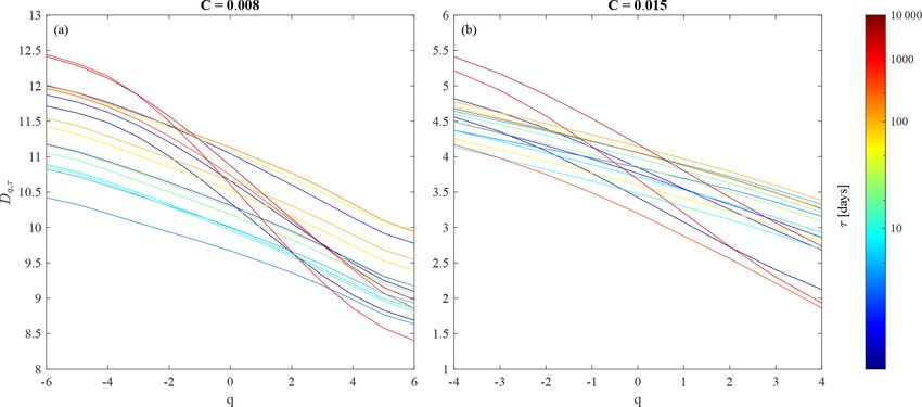
T. Alberti et al.: Multivariate analysis of a reduced order ocean–atmosphere model                                              839

2   The reduced order ocean–atmosphere model                           dynamics with stronger LFV in both the ocean and the atmo-
                                                                       sphere (related to the development of a coupled mode) for
                                                                       larger values of C.
Reduced order coupled ocean–atmosphere models are key
tools in the hierarchy of climate models, allowing for an ex-
tensive analysis of the features of the coupled dynamics that          3   Methods
would otherwise be impossible to evaluate (Lorenz, 1984;
Nese and Dutton, 1993; Roebber, 1995; Jin, 1996; Timmer-               Traditional multivariate and/or spatiotemporal data analysis
mann et al., 2003; Van Veen, 2003; De Cruz et al., 2016;               methods are commonly based on fixing an orthogonal de-
Vannitsem, 2017). These models allow for obtaining key in-             composition basis, satisfying certain mathematical properties
sights into the role of coupling for the development of LFV            such as linearity and/or stationarity (Chatfield, 2016). How-
in the atmosphere associated with the presence of the ocean.           ever, these conditions are not usually met when real-world
   Recently, dynamical analysis has been conducted by                  geophysical data are analyzed, which calls for more adap-
means of the development of a suitable reduced order model             tive methods (Huang et al., 1998). Indeed, adaptive meth-
of the coupled ocean–atmosphere system. This model has                 ods can be helpful for overcoming some limitations of fixed-
been developed starting from the quasi-geostrophic equa-               basis methods, which implicitly assume that a given nat-
tions describing the interaction between a two-layer at-               ural phenomenon or a superposition of physical processes
mosphere and a one-layer ocean over an infinitely deep                 can be represented in terms of a priori defined mathemati-
quiescent ocean layer (Vannitsem et al., 2015; Vannitsem,              cal functions like sine and/or cosine or some other kinds of
2015, 2017; De Cruz et al., 2016, 2018). The ocean flow                wave functions (Chatfield, 2016). Since this cannot be as-
passively advects the temperature within the ocean, while              sured, adaptive methods (as the MEMD) could be more suit-
momentum, radiative, and heat transfer mechanisms realize              able for reducing some mathematical assumptions and a pri-
the coupling between the atmosphere and the ocean. By ex-              ori constraints (Huang et al., 1998; Huang and Wu, 2008;
panding the solutions of these equations into Fourier series,          Rehman and Mandic, 2010). Moreover, geophysical data are
by truncating them at low wavenumbers, and by projecting               usually also characterized by scale-invariant features over a
onto the Fourier modes retained, a set of ordinary differen-           wide range of scales with different complexity and show a
tial equations is derived. The fields are defined over a rect-         scale-dependent behavior due to several factors like forcings,
angular domain with 0 ≤ x ≤ 2π L/n and 0 ≤ y ≤ π L, with               coupling, intrinsic variability, and so on (e.g., Lovejoy and
n denoting the aspect ratio between the meridional and the             Schertzer, 2013; Franzke et al., 2020). For the above rea-
zonal extents of the domain and L the characteristic spatial           sons, in this work we put forward a novel approach based on
scale. Moreover, periodic boundaries along the zonal direc-            combining two different data analysis methods for investi-
tion and free slip along the meridional direction are chosen           gating the multiscale fractal behavior of the coupled ocean–
for the atmosphere, while a closed basin with no flux through          atmosphere system: multivariate empirical mode decompo-
the boundaries is imposed for the ocean.                               sition (MEMD; Rehman and Mandic, 2010) and generalized
   In the reduced order coupled model version proposed in              fractal dimensions (Hentschel and Procaccia, 1983). One of
Vannitsem et al. (2015), a long-periodic attracting orbit com-         the main advantages of combining the MEMD with general-
bining atmospheric and oceanic variables emerges from a                ized fractal dimensions instead of classical approaches deals
Hopf bifurcation for large values of the meridional gradient           with the limited number of intrinsic components that can
of radiative input and frictional coupling. Beyond a certain           be also visually inspected. Indeed, if we, for example, use
value of the meridional gradient for the radiative input, a            Fourier decomposition we will have a large number of (har-
chaotic behavior appears, which is still dominated by LFV              monic) oscillating components at different fixed frequencies
on decadal and multi-decadal timescales.                               that should be summed up for exploiting our proposed proce-
   Here we use the original version of the model (Vannit-              dure. Furthermore, if we, for example, use wavelets we will
sem et al., 2015) where the four relevant fields, i.e., the            deal with some a priori assumptions on the decomposition
barotropic and baroclinic atmospheric streamfunctions, the             basis onto which we are projecting our data that could pro-
ocean streamfunction        and the
                                  Pocean    temperature,
                                                       P8are given     duce misleading results in our procedure of evaluating frac-
by ψa = 10                          10
           P
                 ψ a,i Fi ,  θa =       θa,i Fi , 9o =   i=1 9o,i φi   tal measures on a priori fixed scales. Another advantage is
           Pi=1                     i=1
and To = 8i=1 To,i φi , where Fi and φi are simplified nota-           that MEMD allows to preserve some intrinsic properties of
tions for the sets of modes used, compatible with the bound-           signals related to the nonlinear and/or non-stationary nature
ary conditions of both the atmosphere and the ocean. The               of processes they are associated with, since the decompo-
parameter values used are the ones given in Figs. 8 and 9              sition is based on the local characteristic scale of the data
of Vannitsem (2017). Depending on the choice of the sur-               in deriving intrinsic components with time-dependent ampli-
face friction coefficient C, different solutions are found with        tudes and phases (Huang et al., 1998; Huang and Wu, 2008;
a highly chaotic dynamics without marked LFV in the atmo-              Rehman and Mandic, 2010). However, we do not question
sphere for small values of C, but a more moderately chaotic            the appropriateness of conventional analysis techniques but

https://doi.org/10.5194/esd-12-837-2021                                                   Earth Syst. Dynam., 12, 837–855, 2021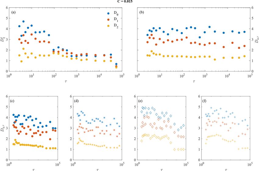
840                                       T. Alberti et al.: Multivariate analysis of a reduced order ocean–atmosphere model

rather acknowledge that other approaches can provide a new                  component-wise to yield multidimensional envelopes
perspective on what we can learn from the respective system                 that are then averaged to obtain the multivariate mean.
under study (Alberti et al., 2020a).
                                                                   This means that the quasi-Monte Carlo method is needed
                                                                   only for selecting a uniform sampling of direction vectors,
3.1   Multivariate empirical mode decomposition (MEMD)
                                                                   thus avoiding implicitly preferred directions that could be
The multivariate empirical mode decomposition (MEMD) is            more dominant with respect to the others, which could in-
the “natural” multivariate extension of the univariate em-         troduce a source of errors in evaluating signal projections
pirical mode decomposition (EMD) (Huang et al., 1998;              (Rehman and Mandic, 2010).
Rehman and Mandic, 2010). MEMD directly works on the                  Having now defined the procedure needed to compute en-
data domain, instead of defining a conjugate space as for          velopes over each direction, the main steps of the sifting pro-
Fourier or wavelet transforms, with the aim of being as            cess acting on a k-variate signal s(t) = [s1 (t), s2 (t), . . ., sk (t)]
adaptive as possible to minimize mathematical assumptions          can be summarized as below:
and definitions (Huang et al., 1998) in extracting embed-
ded structures in the form of so-called multivariate intrin-         1. identify local extremes (i.e., data points where abrupt
sic mode functions (MIMFs) (Rehman and Mandic, 2010).                   changes in the local tendency of the series under study
Each MIMF is an oscillatory pattern of the multivariate co-             are observed);
ordinates having the same number (or differing at most by            2. interpolate local extremes separately by cubic splines
one) of local extremes and zero crossings, and whose up-                (i.e., produce continuous functions with smaller error
per and lower envelopes are symmetric (Huang et al., 1998;              than other polynomial interpolation);
Rehman and Mandic, 2010). MIMFs are derived through the
sifting process (Huang et al., 1998). This process is easily         3. derive the upper and lower envelopes u(t) and l(t), re-
realized for univariate signals (Huang et al., 1998), while             spectively;
it needs to be carefully implemented for multivariate pro-                                                                 u(t)+l(t)
cesses (Rehman and Mandic, 2010), since it is based on               4. derive the mean envelope m(t) as m(t) =                2     ;
the cubic spline interpolation of local extremes that cannot         5. evaluate the resulting candidate MIMF as h(t) = s(t) −
easily be defined on a k-dimensional space (Rehman and                  m(t).
Mandic, 2010). Rehman and Mandic (2010) proposed an
alternative definition of local extremes for multivariate sig-     The previous steps are iteratively repeated until the obtained
nals by considering the k-variate data as composed by k-           candidate MIMF h(t) can be identified as a multivariate
dimensional signals projected onto appropriate directions in       intrinsic mode function (also called multivariate empirical
this k-dimensional space. This allows us to perform cubic          mode) (Huang et al., 1998; Rehman and Mandic, 2010),
spline interpolation in each direction, with the suitable direc-   while the full sifting process ends when no more MIMFs
tions chosen by means of a combination of a quasi-Monte            cj (t) can be filtered out from the data. Hence, we can write
Carlo-based low-discrepancy sequences and a uniform an-
                                                                             Nj
gular sampling method (Rehman and Mandic, 2010). These                       X
allow providing a more uniform set of direction vectors over       s(t) =           cj (t) + r(t).                                       (4)
                                                                             j =1
which to compute the local mean of envelopes, without intro-
ducing any smoother dynamics in the data, via the following        In this way a multivariate signal is decomposed into Nj k-
procedure:                                                         dimensional functions, each containing the same frequency
 1. Given a k-dimensional space we need to find the direc-         distribution, e.g., into a set of k-dimensional embedded os-
    tion vectors by considering that these reduce to points        cillating patterns cj (t) which form the multivariate decom-
    in a (k − 1)-dimensional space.                                position basis, plus a multivariate residue r(t).
                                                                      For each MIMF we can define a k ? -variate mean timescale
 2. The simplest choice is to employ uniform angular sam-          as
    pling on a k-dimensional hypersphere, but this will lead
    to a non-uniform filling of the k-dimensional space (a                          ZT
                                                                              1
    higher density of points would be observed near the            τj,k ?   =            t 0 cj,k ? (t 0 )dt 0 ,                         (5)
    poles).                                                                   T
                                                                                    0

 3. A quasi-Monte Carlo method is used to provide a more           representing the typical oscillation scale of the j th mode for
    uniform distribution of direction vectors.                     the k ? th univariate component cj,k ? extracted from the mul-
 4. Once the direction vectors are chosen, the signal is           tivariate signal sk ? (t) for k ? ∈ [1, k]. Similarly, by ensemble
    projected onto these vectors, the extrema of the re-           averaging over the k-dimensional space we can introduce the
    sulting projected signals are evaluated and interpolated       concept of a multivariate mean timescale as

Earth Syst. Dynam., 12, 837–855, 2021                                                            https://doi.org/10.5194/esd-12-837-2021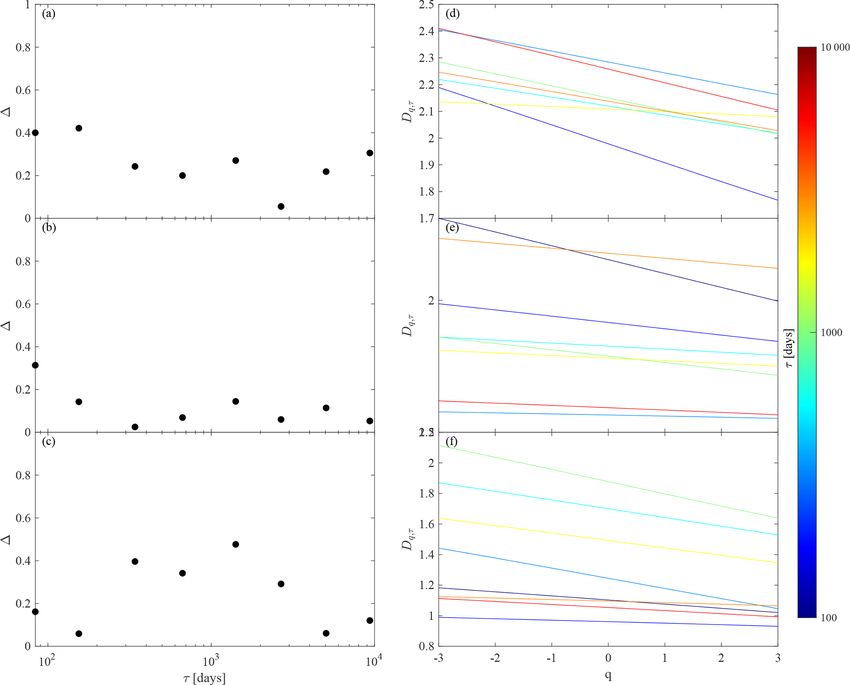
T. Alberti et al.: Multivariate analysis of a reduced order ocean–atmosphere model                                                                         841

                                                                                             with h· · ·i representing a steady-state average operation and δ
           ZT                                                                                indicating a fluctuation at scale τ . For any given τ we can in-
       1                                                                                     troduce a local natural probability measure dµτ such that the
τj =            t 0 hcj (t 0 )ik dt 0 ,                                               (6)
       T                                                                                     probability pi of visiting the ith hypercube Bs ∗ ,τ (`) of size
           0
                                                                                             ` centered at the point s ∗ on the considered (d-dimensional)
with h· · ·ik denoting an ensemble average over the k-                                       phase space of s 1 (t) can be defined as
dimensional space. Thus, the k ? -variate timescale τj,k ? is                                           Z
                                                                                                 .
evaluated for each mode and for each k ? -dimensional data,                                  pi =              dµτ .                                     (10)
while the multivariate mean timescale τj is the mean over all                                     s 1 ∈Bs ∗ ,τ (`)
k ? ∈ (1, k]. Moreover, as for univariate EMD (Huang et al.,
1998), we can introduce the concepts of instantaneous am-                                    By defining a qth order partition function
plitudes a j (t) and phases φj (t) of each MEMD mode via
                                                                                                                     X q Z
the Hilbert transform along the different directions of the k-                               0q (µτ , Bs ∗ ,τ (`)) =  pi = dµτ (s)µτ (Bs ∗ ,τ (`))q        (11)
dimensional space. The instantaneous energy content is then                                                            i
derived as Ej (t) = a j (t)2 . Thereby, we can characterize the
spectral content by introducing an alternative yet equivalent                                and taking the limit ` → 0, the multiscale generalized fractal
definition of the power spectral density (PSD) as                                            dimensions are derived as
                                                                                                         1       log 0q (µτ , Bs ∗ ,τ (`))
                 ZT                         ZT                                               Dq,τ =          lim                           .               (12)
        1                                                              .                               q − 1 `→0         log `
S(τ ) = 2             hEj (t 0 )ik dt 0 ·        t 0 hcj (t 0 )ik dt 0 = σ 2 (τ ) · τ, (7)
       T
                 0                          0                                                Here we identify the intrinsic oscillations by using the
                                                                                             MEMD, and then we investigate the phase-space properties
with σ 2 (τ ) being the k-variate variance of MIMFs and τ the                                at different scales by deriving the generalized dimensions
mean timescale defined as in Eq. (6). Moreover, from the in-                                 (Alberti et al., 2020a). We summarize this process as follows:
stantaneous energy content Ej (t) the relative contribution ej
can be derived as                                                                             1. We extract multiscale components from s(t) by using
                                                                                                 the MEMD.
           1 T        0     0
             R
          T 0 hEj (t )ik dt                                                                   2. We evaluate the intrinsic scale τj of each MIMF.
e j = PN                          .                        (8)
           j 1 T
                R
                         0      0
         j =1 T 0 hEj (t )ik dt                                                               3. We evaluate reconstructions of modes by means of
Finally, as for the univariate decomposition (Huang et al.,                                      Eq. (4):
1998), also the MIMFs are empirically and locally orthogo-                                                               j      ?
nal with respect to each other, the decomposition basis is a
                                                                                                  X                      X
                                                                                                   δs τ (t) → Fj ? (t) =   cj (t),                         (13)
complete set (Rehman and Mandic, 2010), and partial sums                                           τ                          j =1
of Eq. (4) can be obtained (Alberti, 2018; Alberti et al.,
2020b).                                                                                           with j ? = 1, . . ., Nj (by construction, MIMFs are or-
                                                                                                  dered from short to long scales, i.e., τj < τj 0 if j < j 0 ).
3.2    Multivariate and multiscale generalized fractal                                        4. We evaluate the generalized dimensions Dq,τ from
       dimensions                                                                                Fj ? (t) for each j ? (i.e., for each scale τj ? ).
The dynamics of complex systems is usually characterized                                      5. We evaluate the singularities and singularity spectrum:
by a multitude of scales whose dynamical features determine
their collective behavior. Nevertheless, vast efforts have been                                         d
                                                                                                  ατ =      (q − 1)Dq,τ                                    (14)
made to determine collective properties of systems (e.g.,                                              dq
Hentschel and Procaccia, 1983), instead of considering to
                                                                                                  fτ = f (ατ ) = qατ − (q − 1)Dq,τ .                       (15)
measure scale-dependent features. Recently, Alberti et al.
(2020a) introduced a new formalism allowing measuring in-
                                                                                                From Eq. (13) we can inspect the local properties of fluc-
formation at different scales by combining a data-adaptive
                                                                                             tuations in terms of the geometry of the phase space, thus
decomposition method and the classical concept of general-
                                                                                             providing a characterization of dynamical features of differ-
ized fractal dimensions. The starting point is that a multivari-
                                                                                             ent regimes and disentangling the different dynamical com-
ate signal manifesting a multiscale behavior can be written
                                                                                             ponents of (possibly) different origin.
as
                                                                                                Our proposed formalism provides a novel way to inves-
              X                                                                              tigate how phase-space properties (geometry, correlations)
s(t) = hsi +      δs τ (t) = s 0 + s 1 (t),                 (9)
                      τ
                                                                                             change when dynamical components at different mean scales

https://doi.org/10.5194/esd-12-837-2021                                                                              Earth Syst. Dynam., 12, 837–855, 2021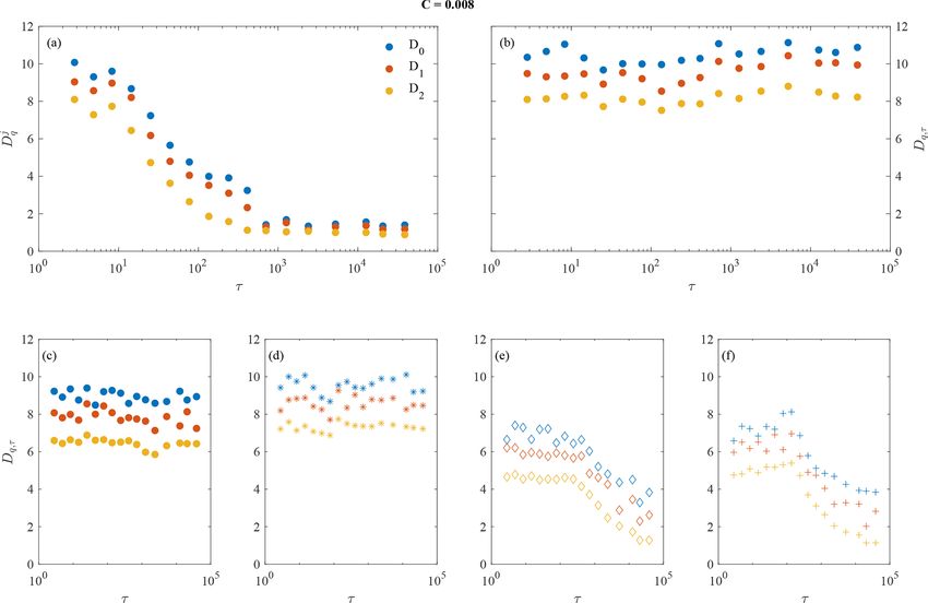
842                                          T. Alberti et al.: Multivariate analysis of a reduced order ocean–atmosphere model

Figure 1. 3-D projection of the full system attractor in the subspace (To,2 , 9o,2 , ψa,1 ) for C = 0.008 (red) and C = 0.015 (black), respec-
tively.

with different dynamics are considered. In other words, we               4     Results
can highlight the role of scale-dependent phenomena in
defining the global properties of a system. Indeed, global               4.1    Multivariate empirical mode decomposition
measures proposed in the past (e.g., Grassberger, 1983;
                                                                         Figure 1 reports the 3-D projection of the full system attractor
Hentschel and Procaccia, 1983) only allow us to investi-
                                                                         in the subspace (To,2 , 9o,2 , ψa,1 ) for two representative val-
gate the statistics of the phase-space scaling properties of the
                                                                         ues of the friction coefficient C (0.008 and 0.015 kg m−2 s−1
whole system; conversely, our proposed approach allows us
                                                                         as indicated by red and black points, respectively). In the fol-
to investigate how the different scales contribute to the global
                                                                         lowing, we will omit the physical units of this parameter for
properties of a system (Alberti et al., 2020a). Moreover, our
                                                                         the sake of brevity. The considered subspace characterizes
framework also provides consistency with established mea-
                                                                         the dynamics of the system as represented by the dominant
sures for characterizing time series from an integral (not
                                                                         mode of the meridional temperature gradient in the ocean
scale-resolved) perspective, since the scale-dependent mea-
                                                                         (To,2 ), by the double-gyre transport within the ocean (9o,2 ),
sures we evaluate converge to the associated global measures
                                                                         and by the vertically averaged zonal flow within the atmo-
as all scales are considered, i.e., when the full system dynam-
                                                                         sphere (ψa,1 ), respectively.
ics, composed by all accessible scales, is reached (Hentschel
                                                                            The behavior of the system is clearly dependent on the
and Procaccia, 1983). Within this framework, our approach
                                                                         friction coefficient, with both the location and the topology
is promising for investigating scale-dependent properties, as
                                                                         of the attractor changing as C is increased from 0.008 (red
measured by fractal dimensions, of the system. Furthermore,
                                                                         points in Fig. 1) to 0.015 (black points in Fig. 1). This be-
since we are indeed interested in nonlinear variability char-
                                                                         havior has also been previously reported by Vannitsem et al.
acteristics at different timescales, employing perfectly linear
                                                                         (2015) and Vannitsem (2015), indicating a drastic qualita-
and/or stationary (harmonic) functions as components would
                                                                         tive change of the nature of the dynamics at about C = 0.011
leave out any information on nonlinear dynamics. Moreover,
                                                                         above which substantial LFV emerges (Vannitsem et al.,
simply looking at the behavior of spectral densities would
                                                                         2015; Vannitsem, 2015, 2017). However, all model com-
leave out any higher-order statistical properties, only focus-
                                                                         ponents are clearly characterized by multiscale variability,
ing on the autocorrelation function (i.e., the second-order
                                                                         spanning a wide range of timescales that can contribute to
moment). By looking at the behavior of fractal dimensions
                                                                         the dynamics in different ways, depending on the values of
we can explore how the different scales contribute to change
                                                                         the friction coefficient and the intrinsic variability of the cou-
the phase-space properties for higher-order statistics (i.e., for
                                                                         pled ocean–atmosphere system.
different values of q).
                                                                            Figure 2 displays the behavior of the spectral energy
                                                                         content S(τ ) of the different MIMFs as a function of
                                                                         their mean timescales τ as in Eq. (7) for the full system
                                                                         (atmosphere+ocean) and for the two subsystems separately
                                                                         (i.e., the atmosphere and the ocean, respectively).

Earth Syst. Dynam., 12, 837–855, 2021                                                         https://doi.org/10.5194/esd-12-837-2021
T. Alberti et al.: Multivariate analysis of a reduced order ocean–atmosphere model 843
Figure 2. Spectral energy content S(τ ) of the different MIMFs as a function of their mean timescales τ as in Eq. (7) for the full system
(atmosphere+ocean, blue circles), only for the atmosphere (orange asterisks), and only for the ocean (yellow diamonds). Panel (a, b) refer
to the two values of the friction coefficient, C = 0.008 and C = 0.015, respectively.
First of all, it is important to underline that a different behaviors can be related to the existence of multiscale vari-
number of MIMFs has been identified for the two different ability of the full system that can be linked to the different
cases: Nj = 17 for C = 0.008 and Nj = 22 for C = 0.015. components operating at different timescales and to the dif-
This underlines that the respective dynamical behavior of the ferent dynamics of the system as the friction coefficient C is
system is different, being characterized by different sets of changed.
empirical modes and consequently by a different number of To further clarify the latter aspect, we evaluate the rel-
relevant timescales. Moreover, by keeping in mind that for ative contribution (in percentage) Eχ,τ of the different
pure noise the expected number of MIMFs is log2 N with N MIMFs (i.e., at different timescales τ ) for each variable
being the number of data points, both situations cannot be χ = {ψa,i , θa,i , 9o,i , To,i } as reported in Fig. 3. It can be
related to a purely stochastic dynamics. Indeed, in both cases clearly noted that the oceanic variability mainly contributes
we have used N = 105 data points; thus the expected num- to the low-frequency dynamics (Eχ,τ > 95 % for χ = {9o,i ,
ber of MIMFs is Njnoise = 16 (Flandrin et al., 2004). How- To,i } and τ &104 d), while the atmosphere is mainly charac-
ever, an interesting feature is that for the lower C value a terized by short-term variability for C = 0.008 (Eχ,τ > 95 %
number of MIMFs closer to that expected for noisy data are for χ = {ψa,i , θa,i } and τ .10 d) and by both short- and long-
found, possibly related to the more irregular dynamics in this term dynamics for C = 0.015. This points towards the C-
low-friction coefficient case. Conversely, a marked departure dependent behavior of the atmospheric dynamics, with the
from Nj = 16 is found for the higher C case, corresponding ocean multiscale variability being less affected by changes
to a more regular dynamics characterized by significant LFV. in the values of the friction coefficient, and to the role of the
Furthermore, from Fig. 2 it is easy to note that the behav- ocean in developing LFV in the atmosphere as C increases.
ior of S(τ ) depends on both the friction coefficient C and the Thanks to the completeness property of the MEMD we
different components of the model. For the full system (i.e., can explore the dynamics of the system as reproduced by the
atmosphere+ocean) S(τ ) decreases as τ increases for both most energetic empirical modes via partial sums of Eq. (4).
values of C, while it is characterized by increasing spectral By using the information coming from the energy percentage
energy content at larger scales (i.e., at lower frequencies). By distribution across the different timescales for each variable
discriminating between the atmospheric and the oceanic con- χ , we can provide MIMF reconstructions accounting for a
tribution we are able to see that (as expected), the short-term certain percentage of energy with respect to the total spec-
variability of the full system can be attributed to the atmo- tral energy content. By ordering the empirical modes with
sphere, while the long-term one is a reflection of the ocean decreasing relative contribution ej and summing up those
dynamics. Moreover, when C increases we note an increase contributing at least 95 % of the total spectral content, we
of the spectral energy content at all timescales, together with are able to investigate the 3-D projection of the full system
a flattening of the atmospheric spectral behavior, while the attractor onto the subspace (To,2 , 9o,2 , ψa,1 ) and compare it
ocean dynamics seems to preserve its spectral features. These with the projection obtained by considering all timescales (as
https://doi.org/10.5194/esd-12-837-2021 Earth Syst. Dynam., 12, 837–855, 2021844 T. Alberti et al.: Multivariate analysis of a reduced order ocean–atmosphere model
Figure 3. Relative contribution (in percentage) Eχ,τ of each variable χ = {ψa,i , θa,i , 9o,i , To,i } in dependence on the mean timescale τ .
Panels (a) and (b) refer to the two values of the friction coefficient C = 0.008 and C = 0.015, respectively. The white line separates the
atmospheric variables from the oceanic ones.
Figure 4. 3-D projection of the full system attractor in the subspace (To,2 , 9o,2 , ψa,1 ) for C = 0.008 (red) and C = 0.015 (black), respec-
tively, as obtained from reconstructions based on the multivariate empirical modes Rχ,95 % (t) accounting for 95 % of the total variance of
the model dynamics.
in Fig. 1). Thus, for each variable χ = {ψa,i , θa,i , 9o,i , To,i }, Table 1. Mode indices j 0 and corresponding k ? -variate timescales
we can define a reconstruction based on empirical modes, τj 0 ,k ? (see Eq. 5) used for the reconstruction based on empirical
Rχ,95 % , as modes Rχ,95 % .
. X
Rχ,95 % (t) = cχ,j 0 (t), (16) C χ j0 τj 0 ,k ? [d]
j 0 |ej 0 ≥95 %
ψa,1 1, 2 3, 5
with cχ,j 0 (t) being the j 0 th
multivariate empirical mode ex- 0.008 9o,2 14, 15, 16 631, 1333, 2086
To,2 14, 15, 16 599, 1132, 1913
tracted via the MEMD of the variables χ. The 3-D projec-
tion onto the subspace (To,2 , 9o,2 , ψa,1 ) of Rχ,95 % is shown ψa,1 21 2690
in Fig. 4, while Table 1 summarizes the mode indices j 0 and 0.015 9o,2 19, 20, 21 829, 1469, 2449
corresponding k ? -variate timescales τj 0 ,k ? (see Eq. 5) used To,2 19, 20, 21 735, 1506, 2598
for the reconstruction.
Earth Syst. Dynam., 12, 837–855, 2021 https://doi.org/10.5194/esd-12-837-2021T. Alberti et al.: Multivariate analysis of a reduced order ocean–atmosphere model 845
Figure 5. Multiscale correlation dimension D2,τ for C = 0.008 at different timescales τj for different cases: (a) for each MIMF individually
j
(D2 ), (b) for reconstructions of MIMFs as in Eq. (12) (D2,τ ), and (c) for reconstructions of MIMFs separately for each variable (barotropic
modes – blue circles, baroclinic modes – orange asterisks, transport modes – yellow diamonds, and temperature modes – violet symbol).
Each panel also shows the 95 % confidence intervals as error bars.
By comparing Figs. 1 and 4 it can be easily noted that the attractor is to compute its spectrum of generalized fractal di-
underlying structure of the 3-D projection of the full attrac- mensions, allowing us to statistically characterize important
tor is essentially the same, thus suggesting that the subspace properties of the dynamics as reflected by its phase-space ge-
statistics of the phase-space scaling information can be re- ometry, including its information content, complexity, and
covered by a subset of multivariate empirical modes. This underlying fractal structure (Grassberger, 1983; Hentschel
underlines that the dynamics of the full system can be re- and Procaccia, 1983; Donner et al., 2011). However, clas-
produced by only few relevant timescales without too much sical approaches can only provide global information on the
loss of information, thus reducing the complexity of the low- phase-space topology (Hentschel and Procaccia, 1983; Ott,
order model itself. These results appear relevant if put into 2002), while multiscale dynamical systems can be charac-
the wider context of coupled ocean–atmosphere dynamics, terized by the statistics of the phase-space scaling changing
allowing us to recover the main features by only considering as different real-space scales are considered (Alberti et al.,
the most relevant (in terms of energy) timescale dynamical 2020a). For this purpose, we investigate the statistics of the
components. phase-space scaling of the coupled ocean–atmosphere model
by evaluating the multiscale generalized fractal dimensions
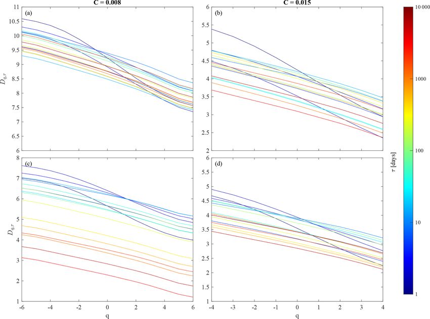
4.2 Multiscale generalized fractal dimensions described in Section 3.2. Figures 5 and 6 report the behavior
of the correlation dimension D2 for both values of the friction
Under general conditions, the complexity of a dynamical sys- coefficient and for three different cases: (a) for each MIMF
tem can be conveniently investigated by means of the nonlin- j
individually (D2 ), (b) for reconstructions of MIMFs (D2,τ ),
ear properties of its phase-space trajectory (e.g., its attractor and (c) for reconstructions of MIMFs performed separately
or repeller in case of dissipative dynamics) (Ott, 2002). One for each variable χ = {ψa,i , θa,i , 9o,i , To,i }.
of the most common ways to characterize the topology of an
https://doi.org/10.5194/esd-12-837-2021 Earth Syst. Dynam., 12, 837–855, 2021846 T. Alberti et al.: Multivariate analysis of a reduced order ocean–atmosphere model Figure 6. Same as in Fig. 5, but for C = 0.015. As expected, the multiscale correlation dimension for each chaotic nature of the system as C increases, together with a MIMF decreases with increasing timescale, being repre- reduced number of degrees of freedom. This points towards sentative of a more regular, less stochastic/chaotic, behav- the possibility of recovering the main features of the model ior of large-scale MIMFs as compared with the short-term with a reduced number of variables and scales. However, the ones (Alberti et al., 2020a). Particularly, when approach- most interesting features emerge when the different variables ing the largest timescales, D2,τ → 1 suggesting the exis- of both atmosphere and ocean are separately investigated by tence of fixed-scale MIMFs, i.e., with the instantaneous fre- means of the multiscale generalized fractal dimensions. It is quencies being almost constant (as expected, e.g., Rehman indeed evident that a scale-independent behavior is found for and Mandic, 2010). Conversely, when the multiscale corre- the atmosphere for both values of C, while a scale-dependent lation dimensions are evaluated by summing up the differ- behavior is observed for the ocean. The former can be easily ent MIMFs, starting from the shortest up to the largest scale, related to the dominant role of the short-term variability for a clearly scale-independent behavior of D2,τ is highlighted the atmosphere, while the latter is a reflection of the long- for both values of the friction coefficient C. This suggests term dynamics of the ocean. Moreover, it is also particularly that the short-term variability mostly defines the correlations interesting to note that higher (lower) D2,τ values are found between pairs of points in the phase space, thus setting the for the atmosphere with respect to the ocean for C = 0.008 minimum number of variables needed to describe the dy- (C = 0.015). This reflects the role of the ocean in developing namics of the system, i.e., its degrees of freedom. However, LFV in the atmosphere as C increases, although the com- the role of C clearly emerges in determining the values of plexity of the full system seems to be determined by the at- D2,τ , being lower for the larger C value. Indeed, D2,τ ∼ 8 mosphere for both C values, being indeed characterized by a for C = 0.008, while D2,τ ∼ 1.5 for C = 0.015. This reflects scale-independent behavior of D2,τ . the different statistics of the attractor scaling of the full sys- The described findings are not only valid for the multiscale tem associated with a different dynamical behavior of the correlation dimension D2,τ but are also observed for both the model variables (Faranda et al., 2019), also suggesting a less multiscale capacity dimension D0,τ and the multiscale infor- Earth Syst. Dynam., 12, 837–855, 2021 https://doi.org/10.5194/esd-12-837-2021
T. Alberti et al.: Multivariate analysis of a reduced order ocean–atmosphere model                                                     847

Figure 7. Multiscale capacity dimension D0,τ , multiscale information dimension D1,τ , and multiscale correlation dimension D2,τ for
                                                                                               j
C = 0.008 at different timescales τj for different cases: (a) for each MIMF individually (Dq ), (b) for reconstructions of MIMFs as in
Eq. (12) (Dq,τ ), and (c–f) for reconstructions of MIMFs separately for each variable (barotropic modes – c, baroclinic modes – d, transport
modes – e, and temperature modes – f).

mation dimension D1,τ as reported in Figs. 7 and 8, together            ocean–atmosphere coupling (i.e., C = 0.015). Although C
with the multiscale correlation dimension D2,τ , for both val-          acts as a control parameter for the dimensionality of the sys-
ues of C.                                                               tem, it is not able to change the underlying fractal nature of
     Our formalism reveals the expected property that for q <           the full system. Indeed, for both C values we clearly observe
q 0 , Dq,τ > Dq 0 ,τ ∀τ (Hentschel and Procaccia, 1983; Alberti         different Dq,τ for different q, thus suggesting the existence
et al., 2020a). Moreover, when evaluating the multiscale gen-           of a multifractal nature of the ocean–atmosphere dynamics
eralized fractal dimensions for each MIMF separately (e.g.,             at all timescales. Furthermore, by separately looking at the
                                             j
Figs. 7a and 8a) a decreasing value for Dq is found as τ in-            two subsystems (i.e., the ocean and the atmosphere) a com-
                       j                                                pletely different behavior emerges (e.g., Figs. 7c–f and 8c–
creases, with all Dq converging towards the same value of
                                   j
1 at large timescales. As for D2 this behavior can be easily            f). In this case, the atmospheric variables are characterized
interpreted in terms of more chaotic vs. more regular MIMFs             by scale-independent Dq,τ , being representative of a high-
when moving from short to large scales. This indeed reflects            dimensional system whose prime dynamics occurs at short
the existence of large-scale MIMFs that are characterized by            timescales and with little effects of large-scale processes on
a linear phase, i.e., a constant timescale (e.g., Rehman and            the collective dynamics of the atmosphere. By contrast, a
Mandic, 2010). Thus, this is a trivial result. Conversely, when         clearly scale-dependent behavior is found for the oceanic
the Dq,τ are evaluated for reconstructions based on MIMFs               variables, with the multiscale generalized dimensions de-
a scale-independent behavior is found for the full system for           creasing at larger timescales, reflecting the effects of large-
both values of C (e.g., Figs. 7b and 8b). However, the key              scale dynamics dominating with respect to the short-term
role of the friction coefficient clearly emerges by looking at          one for the ocean variability. Again the friction coefficient C
the larger values of Dq,τ for C = 0.008 with respect to the             controls the values of Dq,τ , decreasing as C increases, while
lower values found for C = 0.015. This clearly indicates the            both the atmosphere and the ocean are clearly characterized
existence of a completely different dynamics between the                by multifractal features at all timescales.
two values of C, where the coupled ocean–atmosphere dy-                    By estimating the Lyapunov spectra (cf. Fig. S11 in the
namics can be interpreted as a higher-dimensional chaotic               Supplement) separately for the ocean and the atmosphere,
system for reduced ocean–atmosphere coupling (i.e., C =                 we obtained that for C = 0.008 the instability is large for the
0.008) as opposed to a lower-dimensional one for a strong               atmosphere with a Lyapunov dimension DL ∼ 10, while for

https://doi.org/10.5194/esd-12-837-2021                                                      Earth Syst. Dynam., 12, 837–855, 2021
848 T. Alberti et al.: Multivariate analysis of a reduced order ocean–atmosphere model
Figure 8. Same as in Fig. 7, but for C = 0.015.
C = 0.015 the instability is weaker for the atmosphere, and properties of the system evolve with the timescale τ . In-
the Lyapunov dimension is slightly larger than 4. Follow- deed, there are ongoing discussions on the fractal structure
ing the Kaplan–Yorke conjecture (Kaplan and Yorke, 1979), of both the atmosphere and the ocean, especially dealing with
the Lyapunov dimension can be used as a proxy of D0 . the short-term variability and in terms of scaling-law behav-
Hence, our results are clearly consistent with the dimension ior and statistics of increments (e.g., Lovejoy and Schertzer,
estimates for the atmosphere. For the ocean, however, there 2013; Franzke et al., 2020).
seems to be a less good agreement, with DL ≈ 2 while we The Dq,τ spectrum is reported in Fig. 9, where colored
found that D0,τ ≈ 4. This quantitative disagreement could be lines correspond to different timescales. It can be observed
related to the fact that the ocean can be viewed as a relatively that for both values of the friction coefficient C, different
stable system perturbed by high-frequency “noise” due to the values of Dq,τ are obtained for different q, with being Dq,τ
atmosphere. Deeper investigations will be devoted to clarify a nonlinear decreasing function of q. This means that the full
this point in future research. system exhibits signatures of multifractality at all timescales,
As a further step, we evaluate the full spectrum of gen- especially at very short and very long timescales. A sim-
eralized fractal dimensions for each MIMF by considering a ple and direct measure of the degree of multifractality1 is
.
wide range of statistical moments q. As suggested in Lovejoy the so-called multifractal width 1 = Dqmin ,τ − Dqmax ,τ . We
and Schertzer (2013) the range of significant moments can be observe (see Fig. 10a, b, black circles) that 1 ≈ 2 for τ ∈
evaluated by means of the tail of the cumulative distribution [τS , τL ] days, while 1 > 2 for both τ < τS and τ > τL , with
function of the data. Indeed, the effect of sample size and its τS ∼ 20 d and τL ∼ 1 year. This behavior could be the reflec-
implications for spurious scaling may be due either to first- tion of processes operating at different timescales for both
or second-order multifractal phase transitions (Lovejoy and the atmosphere (at short timescales) and the ocean (at long
Schertzer, 2013). To mitigate these effects (e.g. Supplement) timescales). In order to further disentangle those processes,
since we deal with the investigation of scale-dependent frac- we also evaluated the full spectra of the generalized multi-
tal dimensions, we evaluate the cumulative statistics at differ- fractal dimensions for each subsystem (i.e., atmosphere and
ent scales and we observe that extreme fluctuations follow a
power law decay leading to the divergence of the sixth-order 1 Another direct measure is the so-called co-dimension of the
and the fourth-order moment for C = 0.008 and C = 0.015,
mean c = d − D0 where d is the dimension of the phase space (e.g.,
respectively. Thus we fix our range of moments −6 < q < 6
Lovejoy and Schertzer, 2013). For the sake of simplicity we prefer
and −4 < q < 4 for C = 0.008 and C = 0.015, respectively. to use here only the multifractal width since it can be easily derived
This analysis allows characterizing how the (multi)fractal from Dq,τ and not to introduce an additional alternative concept.
Earth Syst. Dynam., 12, 837–855, 2021 https://doi.org/10.5194/esd-12-837-2021T. Alberti et al.: Multivariate analysis of a reduced order ocean–atmosphere model 849 Figure 9. Dq,τ spectra for the coupled ocean–atmosphere dynamics at different timescales τj (indicated by different line colors) for recon- structions of MIMFs as in Eq. (12) (Dq,τ ) for (a) C = 0.008 and (b) C = 0.015. Figure 10. Multifractal width 1 at different timescales τj for reconstructions of MIMFs as in Eq. (12) (Dq,τ ) for (a) C = 0.008 and (b) C = 0.015. The different colors refer to the full system (atmosphere+ocean, black circles), only the atmosphere (red circles), and only the ocean (green circles), respectively. ocean) individually. For both values of C, the corresponding suggests that the presence of strong multifractality in the full results are shown in Fig. 11. system can be essentially attributed to the atmosphere, with We clearly see that for the atmosphere, there is a scale- only a marginal role of the ocean variability in determining independent behavior of Dq,τ for all q, rendering the differ- the fractal structure of the full system. By evaluating the dif- ent curves almost invariant with respect to the scale. By con- ference between Dqmin ,τ and Dqmax ,τ , we can clearly see that trast, a scale-dependent behavior emerges for the ocean for larger values, of the order of 3, are found for the atmosphere, the lower value of C. Indeed, it is evident that as the timescale at almost all timescales (and especially at shorter timescales), increases the multiscale generalized dimensions tend to de- for both values of C. Conversely, larger values are found at crease for all values of q, moving from Dq,τ1 ∈ [5, 8] to shorter timescales for both values of C for the ocean. As Dq,τ17 ∈ [2, 3] for C = 0.008. Conversely, although there is the timescale increases, this difference tends to be reduced an overall reduction in the Dq,τ values for C = 0.0015 with to values close to 1, suggesting a reduced multifractality of respect to those evaluated for C = 0.008, the decrease with the ocean with respect to the atmosphere, especially for the the timescale is less evident for this higher C value, although lower value of C at larger timescales when the role of the it is still present for τ > 1 year (see orange and red curves ocean becomes dominant as compared to the atmosphere (see in comparison with the blue ones in Fig. 11d). This clearly Fig. 2). https://doi.org/10.5194/esd-12-837-2021 Earth Syst. Dynam., 12, 837–855, 2021
850                                          T. Alberti et al.: Multivariate analysis of a reduced order ocean–atmosphere model

Figure 11. Dq,τ spectra for the dynamics of atmosphere and ocean individually at different timescales τj (indicated by different line colors)
for reconstructions of MIMFs as in Eq. (12) (Dq,τ ) for (a, c) C = 0.008 and (b, d) C = 0.015. Panels (a, b) refer to the atmosphere, (c, d) to
the ocean.

4.3   Comparison with regional averages from reanalysis                   225◦ E] and φ ∈ [25, 60◦ N], and the tropical Pacific re-
      data                                                                gion, corresponding to λ ∈ [165, 225◦ E] and φ ∈ [25◦ S,
                                                                          25◦ N] (Vannitsem and Ekelmans, 2018). The individual
As a final step we compare our previous results for the re-               series for the two extratropical regions have been de-
duced order coupled ocean–atmosphere model with those                     rived by projecting the reanalysis  √ fields on two dom-
obtained from reanalysis data (Poli, 2015). More specif-                  inant Fourier modes: (i) F1 =      2 cos πy/Ly and (ii)
ically, we use three different sets of regional time se-                  φ2 = 2 sin (π x/Lx ) sin 2πy/Ly (Vannitsem and Ekelmans,
ries based on the European Centre for Medium-range                        2018). For the tropical Pacific region, the series are formed
Weather Forecasts (ECMWF) ORA-20C project (De Bois-                       by spatial averages. In this way, we obtain two sets of three
séson and Balmaseda, 2016; De Boisséson et al., 2017)                     time series each for both the North Atlantic and the North
that is a 10-member ensemble of ocean reanalyses cover-                   Pacific (i.e., one for the atmosphere and two for the ocean),
ing the complete 20th century using atmospheric forcing                   as well as a third set of three time series for the tropical Pa-
from the ERA-20C reanalysis (https://www.ecmwf.int/en/                    cific (two for the atmosphere at two different pressure levels
forecasts/datasets/reanalysis-datasets/era-20c). Here, we fo-             and one for the ocean). This allows us to build a 3-D pro-
cus on data from January 1958 to December 2009 at monthly                 jection of the local atmosphere–ocean coupled dynamics for
resolution in terms of different monthly averaged time series,            each region (see Vannitsem and Ekelmans, 2018, for more
the set of data also used previously in Vannitsem and Ekel-               details).
mans (2018). This period has been chosen in the latter study                 By using the MEMD analysis to investigate the multivari-
because of the ocean reanalysis dataset showing here smaller              ate patterns of reanalysis data, we found the same number
uncertainties than during the first half of the 20th century              of Nj = 9 MIMFs for each region, whose mean timescales
(De Boisséson and Balmaseda, 2016).                                       range from ∼ 2 months up to ∼ 20 years, suggesting the ex-
   Three different representative regions are chosen: the                 istence of multiscale variability over a wide range of scales.
North Atlantic region, corresponding to the domain de-                    As for the reduced order model, we first investigate the
fined by λ ∈ [55, 15◦ W] and φ ∈ [25, 60◦ N], the North Pa-               behavior of the spectral energy content S(τ ) of the differ-
cific region, i.e., a spherical–rectangle domain with λ ∈ [165,

Earth Syst. Dynam., 12, 837–855, 2021                                                         https://doi.org/10.5194/esd-12-837-2021
T. Alberti et al.: Multivariate analysis of a reduced order ocean–atmosphere model 851
Figure 12. Spectral energy content S(τ ) of the different MIMFs as a function of their mean timescales τ as in Eq. (7) for the North Atlantic
(blue circles), the North Pacific (orange asterisks), and the tropical Pacific (yellow diamonds).
ent MIMFs as a function of their mean timescales τ as in On one hand, both the North Atlantic and the North Pa-
Eq. (7) for the three different regions as shown in Fig. 12. We cific regions (see Fig. 13d, e) are characterized by a scale-
clearly observe an increase of the spectral energy content up dependent behavior, with decreasing Dq,τ as τ increases.
to a timescale τ ∼ 1 year for all regions, then declining for Moreover, by looking at the multifractal width as a function
both the North Atlantic and the North Pacific. Conversely, of the scale (Fig. 13a, b) we find evidence for a decreasing
the tropical Pacific is characterized by larger spectral con- 1 as τ increases, being representative of a transition from
tent also for timescales larger than 1 year, up to τ ∼ 5 years, a short-term multifractal nature to a long-term monofractal
which coincide with the typical timescales of the El Niño– one. These features can be interpreted in terms of the differ-
Southern Oscillation (ENSO). Furthermore, for all regions ent multiscale dynamical processes affecting the atmosphere
a decreasing spectral energy content is found at the largest on short scales and the ocean on larger scales.
timescales (i.e., τ > 5 years). On the other hand, by looking at the tropical Pacific region
To further compare our above model results with those we clearly see an enhancement of 1, i.e., the emergence of
obtained for the reanalysis data, we evaluate the multiscale multifractal features (see Fig. 13c), at annual/multi-annual
generalized fractal dimensions for the three different regions. timescales (i.e., τ ∼ 1–8 years), being also characterized by
.
For each region, we derive both the multifractal width 1 = the largest values of the multiscale generalized fractal dimen-
Dqmin ,τ − Dqmax ,τ and the full multiscale multifractal spec- sions (see Fig. 13f). This could be related to the role of the
trum at different timescales τj for reconstructions of MIMFs El Niño–Southern Oscillation (ENSO) cycle manifesting at
as in Eq. (12) (Dq,τ ). Figure 13 shows the corresponding re- these timescales (between 2 and 7 years), which is likely re-
sults for the North Atlantic region, the North Pacific region, sponsible for the different scale-dependent behavior of Dq,τ
and the tropical Pacific region. as compared to the two other extratropical regions.
First of all, it is important to underline that the multiscale In summary, by means of the reanalysis data, we have been
generalized fractal dimensions are clearly different with re- able to demonstrate that (i) the reduced order coupled ocean–
spect to those obtained from the ocean–atmosphere model. atmosphere model and the reanalysis data show some quali-
This directly follows from the different numbers of variables tatively similar behavior of the multiscale generalized fractal
(time series) in the model, being a 36-dimensional dynam- dimensions, although they are characterized by different ab-
ical system, with respect to the reanalysis data, being a 3- solute values due to the different numbers of variables con-
dimensional projection of the regional ocean–atmosphere dy- sidered in the model and the projections on a few modes of
namics. Nevertheless, although different in terms of absolute the reanalysis data, and that (ii) interesting features emerge
values, both the model and the reanalysis data show a simi- when looking at the scale dependency of the statistics of the
lar qualitative behavior with varying scale τ , although some phase-space scaling for different regions, being the reflec-
differences are found between the different regions. tion of different driving mechanisms and processes operat-
https://doi.org/10.5194/esd-12-837-2021 Earth Syst. Dynam., 12, 837–855, 2021You can also read