Atmospheric Erosion by Giant Impacts onto Terrestrial Planets
←
→
Page content transcription
If your browser does not render page correctly, please read the page content below
Draft version July 22, 2020
                                                 Typeset using LATEX twocolumn style in AASTeX63

                                                      Atmospheric Erosion by Giant Impacts onto Terrestrial Planets
                                                                       J. A. Kegerreis,1 V. R. Eke,1 R. J. Massey,1 and L. F. A. Teodoro2, 3
                                                                      1 Institutefor Computational Cosmology, Durham University, Durham, DH1 3LE, UK
                                                                                  2 BAERI/NASA Ames Research Center, Moffett Field, CA, USA
                                                                       3 School of Physics and Astronomy, University of Glasgow, G12 8QQ, Scotland, UK
arXiv:2002.02977v3 [astro-ph.EP] 20 Jul 2020

                                                                         (Received 20202 February 7; Revised 2020 May 27; Accepted 2020 May 28)

                                                                                                       ABSTRACT
                                                         We examine the mechanisms by which atmosphere can be eroded by giant impacts onto Earth-like
                                                       planets with thin atmospheres, using 3D smoothed particle hydrodynamics simulations with sufficient
                                                       resolution to directly model the fate of low-mass atmospheres. We present a simple scaling law to es-
                                                       timate the fraction lost for any impact angle and speed in this regime. In the canonical Moon-forming
                                                       impact, only around 10% of the atmosphere would have been lost from the immediate effects of the
                                                       collision. There is a gradual transition from removing almost none to almost all of the atmosphere for
                                                       a grazing impact as it becomes more head-on or increases in speed, including complex, non-monotonic
                                                       behaviour at low impact angles. In contrast, for head-on impacts, a slightly greater speed can sud-
                                                       denly remove much more atmosphere. Our results broadly agree with the application of 1D models
                                                       of local atmosphere loss to the ground speeds measured directly from our simulations. However, pre-
                                                       vious analytical models of shock-wave propagation from an idealised point-mass impact significantly
                                                       underestimate the ground speeds and hence the total erosion. The strong dependence on impact angle
                                                       and the interplay of multiple non-linear and asymmetrical loss mechanisms highlight the need for 3D
                                                       simulations in order to make realistic predictions.

                                                       Keywords: Impact phenomena (779); Planetary atmospheres (1244); Earth atmosphere (437); Hydro-
                                                                 dynamical simulations (767).

                                                                 1. INTRODUCTION                                 consequences of giant impacts onto planets like the early
                                                 Terrestrial planets are thought to form from tens of            Earth.
                                               roughly Mars-sized embryos that crash into each other               Our own planet is a compelling example, since we can
                                               after accreting from a proto-planetary disk (Chambers             both observe an atmosphere that has survived to the
                                               2001). At the same time, planets grow their atmo-                 present day and be confident that a giant impact took
                                               spheres by accreting gas from their surrounding neb-              place late in its evolution – creating the Moon in the pro-
                                               ula, degassing impacting volatiles directly into the at-          cess. Several different Moon-formation scenarios have
                                               mosphere, and outgassing volatiles from their interior            been proposed and revised, but no simulations have yet
                                               (Massol et al. 2016).                                             resolved a crust, ocean, or atmosphere for the proto-
                                                 For a young atmosphere to survive it must withstand             Earth (e.g. Lock et al. 2018; Ćuk & Stewart 2012).
                                               radiation pressure of its host star, frequent impacts of            Focusing on the atmosphere, the Earth’s volatile
                                               small and medium impactors, and typically at least one            abundances are remarkably different from those of chon-
                                               late giant impact that could remove an entire atmo-               drites (Halliday 2013), which act as a record of the con-
                                               sphere in a single blow (Schlichting & Mukhopadhyay               densable components of the early Solar System. Specif-
                                               2018). In this paper, we focus on the direct, dynamical           ically, nitrogen and carbon are depleted compared with
                                                                                                                 hydrogen, which could be explained by the loss of N2
                                                                                                                 and CO2 with an eroded atmosphere while retaining
                                               Corresponding author: Jacob Kegerreis                             H2 O in an ocean (Sakuraba et al. 2019). Unlike the
                                               jacob.kegerreis@durham.ac.uk                                      abundances, the isotope ratios match those of primor-
                                                                                                                 dial chondrites. Hydrodynamic escape – driven by XUV
2                                                  Kegerreis et al.

radiation from the star or heat from the planet below –      of head-on collisions of large super-Earths targeted at
preferentially removes lighter isotopes, while impacts re-   explaining a specific exoplanet system (Liu et al. 2015),
move bulk volumes of atmosphere. This suggests that          and another with highly grazing impacts that do not
impacts (not necessarily giant ones) are the primary         interact the solid layers of the planets (Hwang et al.
loss mechanism, driving fractionation by removing more       2018). This leaves serious gaps in our understanding
atmosphere than ocean while preserving isotope ratios        of the formation and atmospheric evolution of planets
(Schlichting & Mukhopadhyay 2018).                           in and outside the Solar System, both in terms of both
   Furthermore, the relative abundances of helium and        lower atmosphere masses and the effect of the impact
neon in different-aged mantle reservoirs suggest that        angle.
the Earth lost its atmosphere on at least two occa-            The aim of this study is thus to begin the exploration
sions (Tucker & Mukhopadhyay 2014). Fractionation            of this almost uncharted parameter space, starting in
of xenon also indicates a complicated history of atmo-       the regime of thin atmospheres. For example: what
spheric loss and the importance of ionic escape in addi-     does the impactor actually do to remove atmosphere in
tion to impact erosion and hydrodynamic escape (Zahnle       different scenarios? How easy it is to partially erode
et al. 2019).                                                some atmosphere as opposed to all or none? And how
   Looking further afield, we have recently learnt not       do these answers change for head-on, grazing, slow, or
only that Earth- to Neptune-mass exoplanets are com-         fast impacts?
mon, but that they host a remarkable diversity of atmo-        Giant impacts are most commonly studied using
spheric masses (Fressin et al. 2013; Petigura et al. 2013;   smoothed particle hydrodynamics (SPH) simulations,
Lopez & Fortney 2014). The stochastic nature of giant        where planets are modelled with particles that evolve
impacts makes them a strong candidate for explaining         under gravity and material pressure. It was recently
some of the differences between planets that would oth-      shown that at least 107 (equal-mass) SPH particles can
erwise be expected to have evolved similarly (Liu et al.     be required to converge on even the large-scale results
2015; Bonomo et al. 2019). Irradiation and photoevap-        from simulations of giant impacts, and that the resolu-
oration from stellar winds can significantly erode an at-    tion requirements for reliable results depend strongly on
mosphere (Lopez et al. 2012; Zahnle & Catling 2017),         the specific scenario and question (Kegerreis et al. 2019;
but not enough to explain the diversity of planets around    Hosono et al. 2017).
dim stars, where it should be much less effective.             Computational advances enable us for the first time
   Previous studies of giant-impact erosion have primar-     to study the erosion of thin atmospheres with full, 3D
ily used analytical approaches and 1D simulations to es-     simulations. In this paper, we present high-resolution
timate atmospheric loss from a range of impact energies      simulations of giant impacts with a variety of impact
(e.g. Genda & Abe 2003; Inamdar & Schlichting 2015).         angles and speeds onto the proto-Earth, hosting a range
The one-dimensional nature of these studies also means       of low atmosphere masses. We study the detailed mech-
that little work has been done on grazing collisions, in     anisms of erosion, compare with previous analytical and
spite of the fact that these are far more likely to oc-      1D estimates, and present a simple scaling law for the
cur. Some studies have investigated oblique impacts for      fraction of lost atmosphere in this regime.
much smaller (of order 10 km) objects (Shuvalov 2009),
in which case the erosion is only ever in the local region                         2. METHODS
and the planet’s curvature is negligible. Their results        In this section we describe the initial conditions for the
showed a strong increase in local loss for more-oblique      model planets, the range of impact scenarios, and the
impacts, which is the opposite of the trend for giant        previous models to which we compare our results. The
impacts (Kegerreis et al. 2018). The typical approach        SPH simulations are run using the hydrodynamics and
for giant impacts is to estimate the ground velocities in-   gravity code SWIFT 1 (Kegerreis et al. 2019; Schaller
duced by the impact to study how much atmosphere is          et al. 2016).
blown away. This misses out the complex details of a
collision that can mix, deform, and remake both an at-                         2.1. Initial Conditions
mosphere and the rest of the planet. Any precise study         As a recognisable starting point, we consider an im-
of the consequences of a giant impact therefore requires     pact similar to a canonical Moon-forming scenario, with
full 3D modelling of the planet and atmosphere at the        a target proto-Earth of mass 0.887 M⊕ and impactor of
same time.
   Recent progress has been made in the regime of thick
                                                               1   SWIFT is in open development and publicly available at
atmospheres by two studies: one with 3D simulations
                                                                   www.swiftsim.com.
Atmospheric Erosion by Giant Impacts                                                         3

mass 0.133 M⊕ . Both are differentiated into an iron core                            vc
and rocky mantle, constituting 30% and 70% of the to-                                                                               i
                                                                           t                                            v
tal mass, respectively, and have no pre-impact rotation.
The radii of the outer edge of the core and mantle are                                    β                                     y
0.49 and 0.96 R⊕ for the target and 0.29 and 0.57 R⊕
for the impactor. We use the simple Tillotson (1962)                                                      x
iron and granite equations of state (EoS) (Melosh 2007,
Table AII.3) to model these materials (Kegerreis et al.
2019) 2 .
                                                                         Figure 1. The initial conditions for an impact scenario,
  For the atmospheres, we use Hubbard & MacFar-                          with the target (t) on the left and the impactor (i) on the
lane (1980)’s hydrogen–helium EoS, as described in                       right, in the target’s rest frame. The angle of first contact,
Kegerreis et al. (2018). This includes a temperature-                    β, is set ignoring the atmosphere and neglecting any tidal
and density-dependent specific heat capacity and an adi-                 distortion before the collision. The initial separation is set
abatic temperature–density relation. An ideal gas would                  by the time to impact, as described in Appx. A.
probably be sufficient for the smaller atmospheres, but
larger ones stray into the more-dense regime that this                      To produce the radial density and temperature pro-
EoS is designed to include.                                              files for each atmosphere mass, the surface temperature
  The Tillotson EoS does not treat phase boundaries                      is kept fixed at 500 K for simplicity while the surface
nor mixed phases correctly but is widely used for SPH                    pressure is varied until the desired atmospheric mass is
impact simulations owing to its computationally conve-                   obtained. In other words, the inner two layer profiles
nient analytical form (Stewart et al. 2019). These limi-                 are integrated inwards from the surface (see Kegerreis
tations could be important for studies that require accu-                et al. 2019, Appx. A), then the atmosphere layer profile
rate modelling of, for example, the thermodynamic state                  is integrated outwards, until reaching a negligible mini-
of low-density material in orbit. However, for the focus                 mum density of 10 kg m−3 . Separately, the total radius
in this paper on the large-scale shock-wave propagation                  is also iterated to obtain the 30:70 mass ratio of iron to
and overall erosion caused by impacts, the details of the                rock.
EoS are not expected to significantly affect the results.                   Particles are then placed to precisely match these pro-
  The atmosphere is adiabatic above a 500 K surface,                     files using the stretched equal-area (SEA) method 3 de-
while the iron and silicate layers are given a simple                    scribed in Kegerreis et al. (2019). This results in a re-
temperature–density relation of T ∝ ρ2 , chosen some-                    laxed arrangement of particles that have SPH densities
what arbitrarily to produce a central temperature of                     within 1% of the desired profile values, mitigating the
∼5000 K similar to the Earth today. Our surface tem-                     need for extra computation that is otherwise required to
perature is lower than the 1500 K of Genda & Abe                         produce initial conditions that are settled and ready for
(2003), but the fact that their erosion results are similar              a simulation.
to those of Inamdar & Schlichting (2015) that used many
thousands of Kelvin suggests that the loss is not highly                                      2.2. Impact Simulations
sensitive to this choice, as we test directly ourselves in                  We specify each impact scenario by the impact pa-
§3.3.                                                                    rameter, b = sin(β), and the speed, vc , at first contact
  We test a range of atmosphere masses on the proto-                     of the impactor with the target’s surface, as illustrated
Earth, namely 10−1 , 10−1.5 , 10−2 , and 10−2.5 M⊕ , as                  in Fig. 1. The initial position of the impactor is set such
the lowest mass that we might expect to resolve ade-                     that contact occurs 1 hour after the start of the simula-
quately with 107 equal-mass SPH particles. The cor-                      tion, to allow for some natural tidal distortion and to not
responding pressure at the base of the atmosphere is                     disrupt the system by suddenly introducing the large im-
5.5, 2.4, 0.92, and 0.32 GPa, respectively. They extend                  pactor right next to the no-longer-in-equilibrium target,
out to a pressure of ∼0.1 MPa at 1.55, 1.27, 1.13, and                   as described in Appx. A. Note that the speed at contact
1.06 R⊕ , respectively. The Earth’s atmosphere today                     is always chosen in units
                                                                                               p of the mutual escape speed of
has a mass of ∼10−6 M⊕ , though it may have been                         the system, vesc = 2G (Mt + Mi ) / (Rt + Ri ), where
much thicker in the past.                                                Rt neglects the thickness of any atmosphere, which is

  2   Note that Appx. B of Kegerreis et al. (2019) has a typo in the       3   The     SEAGen        code     is   publicly available at
      sign of du = T dS − P dV = T dS + (P/ρ2 ) dρ just after Eqn. B1.         github.com/jkeger/seagen and the python module seagen
                                                                               can be installed directly with pip.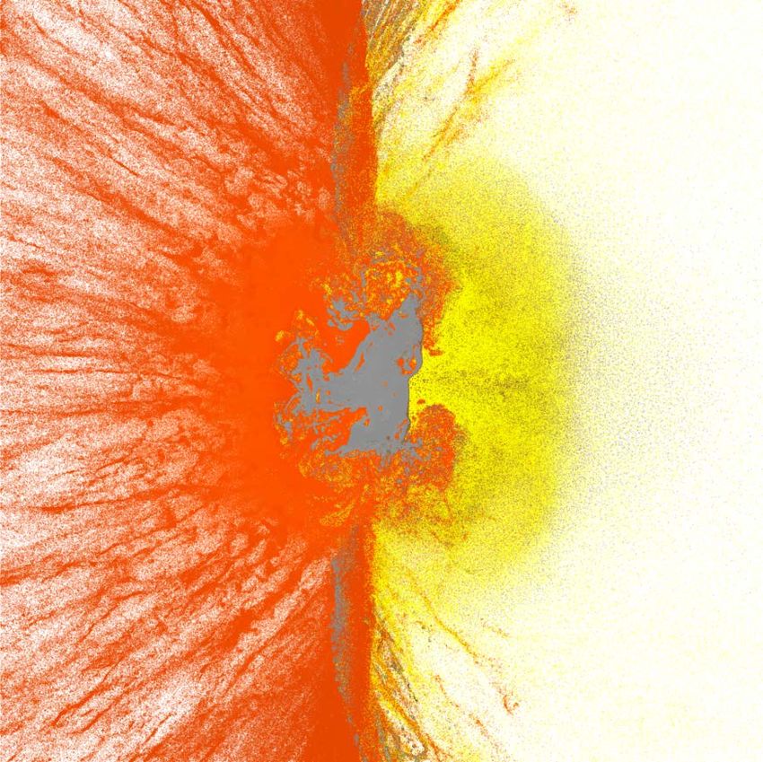
4 Kegerreis et al.
1.0 90
parameter space and is a regime that could be more
60 common in other planetary systems, for example with a
0.8 more massive star or a target planet deeper in the star’s
Impact Parameter, b
Impact Angle, β (◦)
45 potential well. Furthermore, in studies like that by In-
0.6 amdar & Schlichting (2015) where erosion is estimated
Matm N as a function of the impactor’s momentum, using very
30
0 106 high velocities will allow us to test the degeneracy be-
0.4 10−2.5 106.5 tween impactor mass and speed across a wide range of
10−2 107 momenta in future suites with different impactor masses.
10−1.5 107.5
15
0.2 For the relatively small impactor mass used here, even
10−1 108
8 vesc is not predicted by Inamdar & Schlichting (2015)
0.0 0 to remove more than 3/4 of the atmosphere.
0 1 2 3 4 5 6 7 8 The simulations are run using SWIFT with a sim-
Speed at Contact, vc (vesc) ple ‘vanilla’ form of SPH plus the Balsara (1995) switch
for the artificial viscosity as described in Kegerreis
Figure 2. The suite of simulation scenarios, arranged by
their speed and impact parameter at contact (see Fig. 1 and
et al. (2019) to a simulation time of 100,000 s (roughly
Appx. A). As shown in the legend, the nested marker colours 28 hours) in a cubic box of side 80 R⊕ to allow the
indicate the mass of the atmosphere (in Earth masses) for tracking of ejecta. Any particles that leave the box
each simulation, while the line angles indicate the number of are removed from the simulation. Throughout the first
particles per Earth mass. 10 hours we record snapshots every 100 s, for high time
resolution during the impact and its immediate after-
slightly faster for the planets with more massive atmo- math. To reduce data storage requirements, we then
spheres (9.1 up to 9.6 km s−1 ). output snapshots every 1000 s for the remainder.
We run a primary suite of 74 simulations with ∼107
SPH particles, plus 10 of these scenarios re-simulated 2.3. Analytical and 1D Models
additionally with 106 , 106.5 , 107.5 , and 108 particles
We use two previous erosion studies for comparison
for convergence tests, plus 12 miscellaneous tests with
with our 3D simulations, both for the resulting loss of
107 particles detailed in §3.3. To be precise, these
atmosphere and for the shock waves caused by the im-
stated particle numbers refer to the number of parti-
pact. Genda & Abe (2003) used 1D models to simulate
cles per Earth mass (the bare target plus impactor mass
the reaction of the atmosphere to a shock from vertical
is 1.02 M⊕ ). Thus, the numerical resolution stays the
ground motion. Their results for the local fraction of
same for simulations with different-mass planets. For
lost atmosphere, Xlocal , are fitted well by a simple lin-
example, a ‘107 ’ simulation that includes a 0.1 M⊕ at-
ear function of the ground speed, vgnd , in units of the
mosphere actually contains a total of ∼1.12×10⁷ parti-
escape velocity: Xlocal = −1/3 + 4/3 (vgnd /vesc ) capped
cles. For most of the suite we focus on the 10−2 M⊕
at zero and one (their Eqn. 17), which they conclude is
atmosphere.
largely insensitive to the initial conditions of the atmo-
Fig. 2 summarises the parameters for each simula-
sphere.
tion. Note that the vc = 0.75 vesc scenarios would re-
Inamdar & Schlichting (2015) performed similar 1D,
quire some third body to have slowed down the impactor
Lagrangian, vertical-shock simulations, but extended
during its approach to below the mutual escape speed.
them to include thicker atmospheres up to 10% of the
This is unlikely in the case of primary impactors falling
solid mass of the planet. They agree with Genda & Abe
in to the Earth in our solar system, but is a useful test
(2003) for thin atmospheres. Schlichting et al. (2015)
for the consequences of a highly grazing impact result-
also created a model for predicting the ground speeds
ing in a large bound fragment that will re-impact at a
caused by a giant impact, by treating the collision as
later time. It also lets us compare with other models,
a point-mass explosion on a spherical planet of con-
which predict little erosion in this regime.
stant density. They assumed momentum conservation
At the high-speed end, given the Earth’s position in
with a uniform speed in the spherical region traversed
the Solar System, 5 vesc is around the highest typical
by the shock front, which leads to the vertical ground
velocity that might be expected for an impact (Ray-
speed as a function of distance, l, from the impact point:
mond et al. 2009). For context, the Earth’s orbital speed
vgnd = vimp (Mi /Mt )[(l/(2Rt ))2 (4 − 3l/(2Rt ))]−1 (their
around the Sun is about 3 vesc . The suite’s extension
Eqn. 28), where vimp is the speed of the impactor and
to 8 vesc both allows us to test the extreme end of the
Rt and Mt are the radius and mass of the target planet.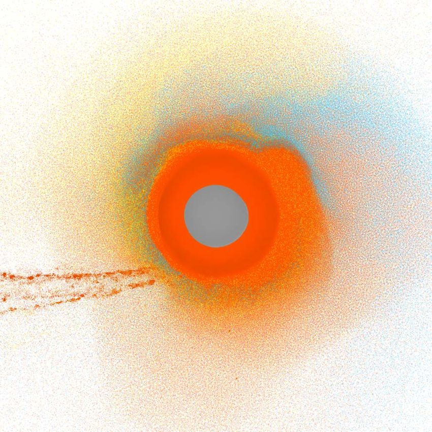
Atmospheric Erosion by Giant Impacts                                          5

                         b = 0, vc = 1        0.1 h                       0.7 h                    3.9 h                    9.5 h
                     2
   y Position (R⊕)

                     0

              −2

                         b =−2
                            0.7, vc = 01     20.1 h      −2       0      21.5 h   −2       0      25.6 h   −2       0      2 h
                                                                                                                          10.9
                              x Position (R⊕)             x Position (R⊕)          x Position (R⊕)          x Position (R⊕)
                     2
   y Position (R⊕)

                     0

              −2

                         b =−2
                            0, vc = 3 0      20.1 h      −2       0      20.3 h   −2       0      23.0 h   −2       0      2 h
                                                                                                                          10.1
                              x Position (R⊕)             x Position (R⊕)          x Position (R⊕)          x Position (R⊕)
                     2
   y Position (R⊕)

                     0

              −2

                         b =−2
                            0.7, vc = 03     20.1 h      −2       0      20.4 h   −2       0      23.0 h   −2       0      27.1 h
                              x Position (R⊕)             x Position (R⊕)          x Position (R⊕)          x Position (R⊕)
                     2
   y Position (R⊕)

                     0

              −2

                            −2       0      2            −2       0      2        −2       0      2        −2       0      2
                             x Position (R⊕)              x Position (R⊕)          x Position (R⊕)          x Position (R⊕)
Figure 3. Illustrative early snapshot cross-sections from the four fiducial impact simulations – head-on and slow, grazing
and slow, head-on and fast, grazing and fast – with b = 0 or 0.7, and vc = 1 or 3 (labelled throughout in units of vesc ), with
the 1% M⊕ atmosphere and ∼108 SPH particles. Grey and orange show the target’s core and mantle material respectively,
and brown and yellow show the same for the impactor. Blue is the target’s atmosphere. The colour luminosity varies slightly
with the internal energy. Note that the snapshots are at different times for each simulation to show the evolution in each case.
The impactors are travelling in the −x direction at the moment they contact the target (see Fig. 1). Animations of the early
evolution of these impacts are available at icc.dur.ac.uk/giant impacts.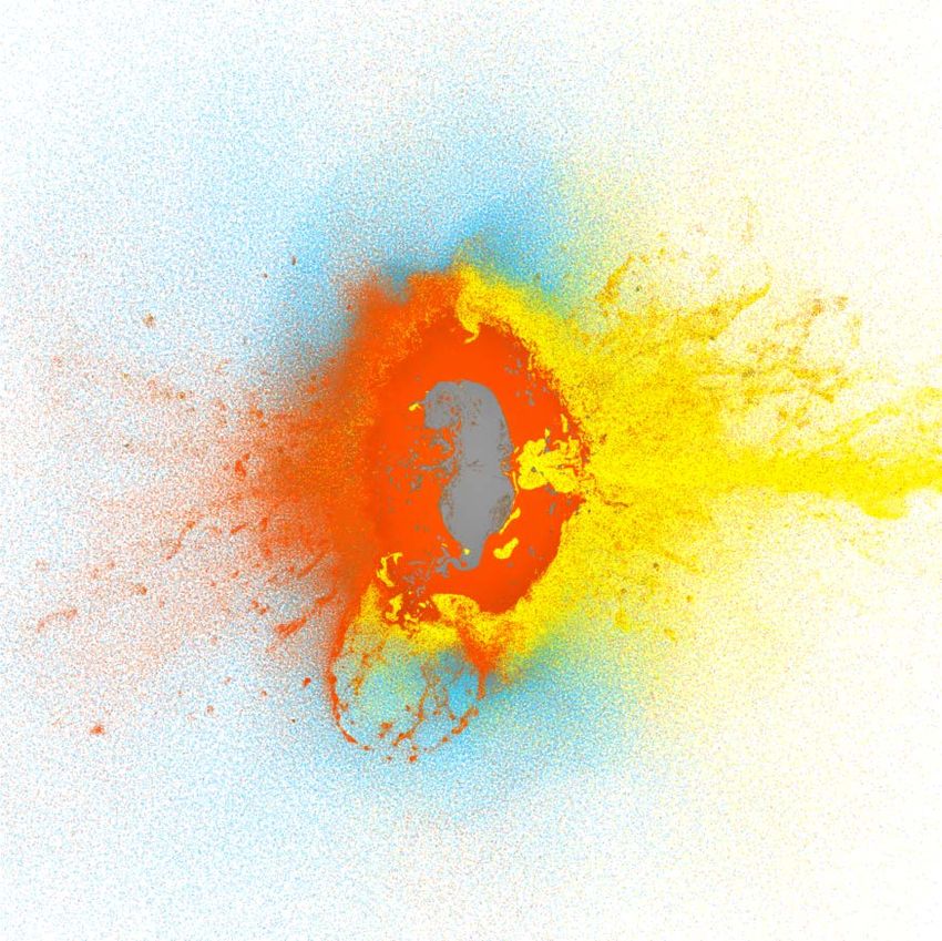
6                                                              Kegerreis et al.

                      b = 0, vc = 1          b = 0.7, vc = 1              b = 0, vc = 3               b = 0.7, vc = 3
               2
    y Position (R⊕)

               0

                      X = 0.150              X = 0.084                    X = 0.997                   X = 0.346
                              0          2           0          2                 0          2                0          2
                           x Position (R⊕)        x Position (R⊕)              x Position (R⊕)             x Position (R⊕)
Figure 4. The particles that will become unbound and escape the system, highlighted in purple on a pre-impact snapshot,
for the four fiducial impacts and our standard ∼107 SPH particles. The other particle colours are muted versions of those in
Fig. 3 as a background for the highlighted ones. Only a thin cross-section of the particles that are within one SPH smoothing
length of z = 0 are shown for clarity. For grazing impacts, higher latitudes may suffer less erosion (see §3.4). The X values give
the total mass fraction of the atmosphere that is lost.

By combining their speed estimates with the 1D lo-                             demonstrated in the high-speed, grazing case (4th
cal erosion model, they presented predictions for the                          row);
global atmospheric mass-loss fraction as a function of
the impactor speed and velocity for different atmosphere                     • The shock wave travelling through the planet from
masses (their Fig. 5).                                                         the impact point, which even erodes some mantle
                                                                               as well in the high-speed, head-on case (3rd row);
                      3. RESULTS AND DISCUSSION
   We begin investigating the simulations with an                            • Subsequent oscillations of the planet, such as the
overview of the general features and consequences of                           plume of impactor mantle in the 3rd snapshot of
these classes of impacts. Then, we focus on the isolated                       the low-speed, head-on case (1st row) – much like
effects of changing the impact parameter, speed, or at-                        the large splash created after dropping a stone into
mosphere mass, and examine the time at which material                          a pond;
is ejected. We consider the ground speeds and localised
loss to compare our results with previous estimates, then                    • The secondary impact of the impactor following
collate all the simulation results to find a simple scaling                    an initial grazing collision, as in the 3rd snapshot
law for the total atmospheric erosion from any scenario                        of the low-speed, grazing case (2nd row).
in this regime.
                                                                         All of these mechanisms may contribute to the total loss
     3.1. General Features of Impacts and Erosion                        in a given scenario. This provides some context with
                                                                         which to consider the rest of the suite and some appre-
  We choose four simulations to act as fiducial compar-
                                                                         ciation for the complexity created by all these processes
isons for the rest of the suite, demonstrating head-on
                                                                         intermingling.
and grazing, slow and fast scenarios. They stand out
                                                                           The particles that are eroded by these four impacts
in Fig. 2 as the impacts for which we simulate multiple
                                                                         are highlighted in Fig. 4, selected by being gravitation-
atmosphere masses and with multiple resolutions. Snap-
                                                                         ally unbound and remaining so until the end of the 105 s
shots from these fiducial simulations are shown in Fig. 3,
                                                                         simulation or until the time the particle exits the 80 R⊕ -
for a target with a 1% M⊕ atmosphere, using ∼108 SPH
                                                                         wide simulation box. The resulting mass fractions of
particles.
                                                                         lost atmosphere are 0.15, 0.08, 1.0, and 0.39, respec-
  In general, the impactor merges with the target for
                                                                         tively. We revisit these final loss results in the context
head-on or slow cases, but may not for fast, grazing
                                                                         of the whole suite after presenting the rest of the simu-
impacts. In addition to any differences in the result-
                                                                         lations and introducing the previous analytical and 1D
ing fraction of lost atmosphere, the timing and cause
                                                                         estimates for comparison. For now, Fig. 4 demonstrates
of loss can also vary significantly with the impact sce-
                                                                         the expected qualitative results following the above dis-
nario. For example, atmosphere may be eroded by – in
                                                                         cussion of Fig. 3: the head-on, slow case loses atmo-
approximately chronological order:
                                                                         sphere around the impact point and the antipode; the
    • Direct encounter with the very-much-not-a-point-                   grazing, slow case shows little antipode erosion, suggest-
      mass impactor passing through, most dramatically                   ing a weaker shock, and primarily loses atmosphere in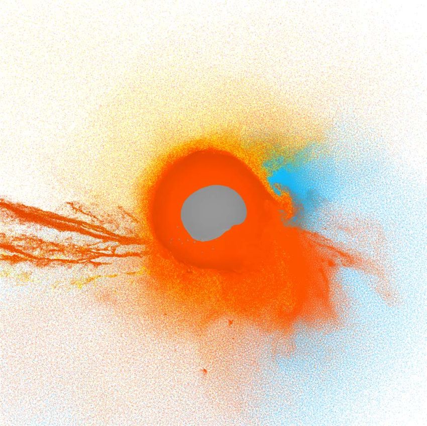
Atmospheric Erosion by Giant Impacts                                           7

                  b = 0, vc = 1         b = 0.3                b = 0.5                b = 0.7                b = 0.9
y Position (R⊕)

           2

           0

                  vc = 3 0       2           0         2            0         2            0         2             0         2
                    x Position (R⊕)       x Position (R⊕)        x Position (R⊕)        x Position (R⊕)         x Position (R⊕)
y Position (R⊕)

           2

           0

                  b = 0, 0vc = 0.75 2   vc = 2 0       2       vc = 3 0       2       vc = 5 0       2       vc = 8 0        2
                    x Position (R⊕)       x Position (R⊕)        x Position (R⊕)        x Position (R⊕)         x Position (R⊕)
y Position (R⊕)

           2

           0

                  b = 0.70       2           0         2            0         2            0         2             0         2
                    x Position (R⊕)       x Position (R⊕)        x Position (R⊕)        x Position (R⊕)         x Position (R⊕)
y Position (R⊕)

           2

           0

                       0         2           0         2            0         2            0         2             0         2
                    x Position (R⊕)       x Position (R⊕)        x Position (R⊕)        x Position (R⊕)         x Position (R⊕)
Figure 5. The particles that will become unbound and escape the system, as in Fig. 4, for example subsets of (top two rows)
different impact parameters and (bottom two rows) different speeds at contact.

the direct path of the impactor; the head-on, fast im-                    core, it gets rapidly forced back out in a random di-
pactor has blasted off almost all the atmosphere and                      rection determined by the arrangement of the discrete
some mantle from the strong shock wave; and the graz-                     particles. In our simulations of the same impact scenario
ing, fast case is similar to the grazing, slow one, but the               using different numbers of particles, the same eruption
impactor has taken some of the mantle in its path along                   of material is produced at the same time, but with dif-
with the atmosphere and blasted away some atmosphere                      ferent random orientations in the y–z plane. On the
around the antipode. The grazing, fast impactor itself                    one hand, this highlights the imperfect symmetry of our
also remains unbound in this hit-and-run collision.                       SPH planets, which prevents the modelling of perfectly
   Note that even head-on collisions are not perfectly ro-                idealised head-on collisions. On the other hand, this also
tationally symmetric in our simulations, because the sys-                 demonstrates the importance of using fully 3D hydrody-
tem is represented using a finite number of particles.                    namical simulations to study realistically chaotic giant
For example, in addition to the large plume of material                   impacts, where we should expect some level of asymme-
ejected during the low-speed, head-on impact, a small                     try and precisely head-on impacts have a probability of
blast occurs on the −y side (1st row in Fig. 3). This                     zero. At any rate, this feature ejects negligible unbound
is impactor material that initially plunges deep into the                 material, so does not affect the overall results of this
target’s centre. Being much less dense than the iron                      specific study.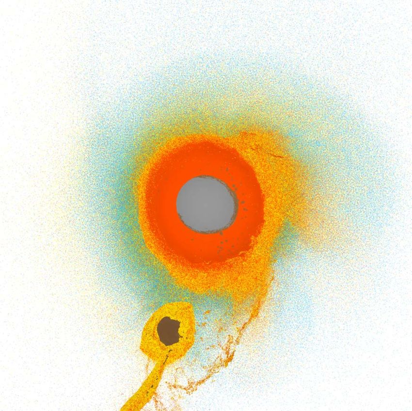
8                                                                                            Kegerreis et al.
                                                                                                           1.0
                                                               vc = 1                           b                vc = 3                         b
                                            0.20
                                                                                                     0                                               0
            Atmosphere Mass Loss Fraction                                                            0.3   0.8                                       0.3
                                                                                                     0.5                                             0.5
                                            0.15                                                     0.7                                             0.7
                                                                                                     0.9   0.6                                       0.9

                                            0.10
                                                                                                           0.4

                                            0.05                                                           0.2

                                                         1.0                                               1.0
                                                                                                    b=0                                        b = 0.7
                         Atmosphere Mass Loss Fraction

                                                         0.8                                               0.8
                                                                                                                                               vc
                                                                                               vc
                                                                                                                                                    0.75
                                                         0.6                                        0.75   0.6                                      1
                                                                                                    1
                                                                                                                                                    2
                                                                                                    2
                                                                                                                                                    3
                                                         0.4                                        3      0.4
                                                                                                                                                    5
                                                                                                    5
                                                                                                                                                    8
                                                         0.2                                               0.2

                                                         0.0                                               0.0
                                                                 0      2        4       6           8             0      2        4       6         8
                                                                            Time (hours)                                      Time (hours)
Figure 6. The early time evolution of the mass fraction of unbound atmosphere for different subsets of impact parameters
and speeds (labelled in units of vesc ) with the 1% M⊕ atmosphere and ∼107 particles. i.e. the times at which the highlighted
atmosphere particles in Fig. 5 become unbound. Note that the vertical axis in the top-left panel does not reach 1. Time = 0 is
set to be the time of contact from Appx. A, 1 hour after the start of the simulation.

  We now turn to the rest of the suite in a similar                                                        For head-on impacts, by vc = 2 vesc , already almost all
manner, continuing this initial overview of general be-                                                    of the atmosphere is eroded. At higher speeds, more
haviour. The top two rows of Fig. 5 highlight the parti-                                                   mantle is also lost, and vc = 8 vesc disintegrates the
cles that become lost from subsets of changing-impact-                                                     planet entirely. The faster grazing impacts can still de-
parameter scenarios, with either the low or high fiducial                                                  liver enough energy to drive some antipodal loss but re-
speeds and the same atmosphere and number of parti-                                                        move systematically less atmosphere than head-on col-
cles. Filling in the gaps between the fiducial examples,                                                   lisions, and even by vc = 5 vesc with b = 0.7 almost half
there is a trend from more global, shock-driven erosion                                                    of the atmosphere still survives.
for low impact parameters, to direct, localised erosion                                                       We find broadly similar behaviour for different masses
for high impact parameters.                                                                                of atmosphere, in simulations with the same fiducial im-
  Fig. 5’s bottom two rows show the eroded particles                                                       pact parameters and speeds. For slow, head-on impacts
from subsets of changing-speed scenarios, with either                                                      onto targets with atmospheres at and below ∼10−2 M⊕ ,
the head-on or grazing fiducial impact parameters. Even                                                    the mantle erosion is similar to the case with zero at-
though the slowest impactors make contact at below the                                                     mosphere. Thicker atmospheres begin to significantly
escape speed, they still erode some atmosphere locally.                                                    cushion the mantle from erosion. The low- and zero-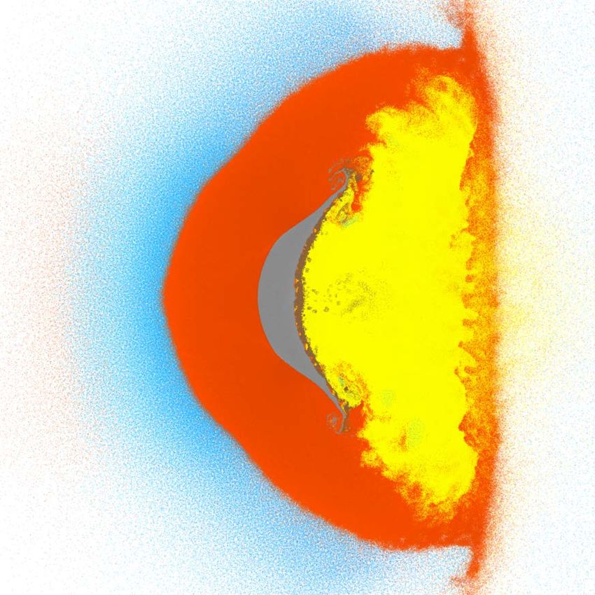
Atmospheric Erosion by Giant Impacts                                                 9

                                                                                                             10−1             106
                                            0.20
                                                                                                             10−1.5           106.5
            Atmosphere Mass Loss Fraction                                                                    10−2             107
                                                                                                             10−2.5           107.5
                                            0.15                                                                              108

                                            0.10

                                            0.05

                                                                                    b = 0, vc = 1                                     b = 0.7, vc = 1
                                                         1.0
                         Atmosphere Mass Loss Fraction

                                                         0.8

                                                         0.6

                                                         0.4

                                                         0.2

                                                                                    b = 0, vc = 3                                     b = 0.7, vc = 3
                                                         0.0
                                                               0   2        4       6       8           0        2         4       6            8
                                                                       Time (hours)                                   Time (hours)
Figure 7. The early time evolution of the mass fraction of unbound atmosphere for the four fiducial impact scenarios with
different atmosphere masses (labelled in units of M⊕ ). Note that the vertical axes in the top panels do not reach 1. The dotted
and dashed lines show the loss evolution for different numbers of particles, as given in the legend.

mass atmosphere cases are also similar in the other three                                           of the planet, shocking away surviving shells of atmo-
fiducial scenarios, although for slow, grazing collisions                                           sphere or even ejecting plumes of material, as seen in
the thicker atmospheres can affect the path of the im-                                              the slow, head-on fiducial example (Fig. 3). For high im-
pactor as it passes through, making the comparison less                                             pact parameters, delayed erosion can also be caused by
direct. At higher speeds, the atmosphere mass makes                                                 the secondary collision of grazing impactor fragments.
less difference, especially in the head-on case, because                                            However, given the low speeds required for a grazing
both any gravitational acceleration and hydrodynami-                                                fragment to return and the likely reduced mass of the
cal deceleration will have smaller effects.                                                         fragment, this has a smaller effect.
                                                                                                      The majority of loss has finished by 4–8 hours after
                          3.2. Erosion Time Evolution                                               contact in all cases, and the eroded mass remains con-
  The time at which the lost atmosphere becomes un-                                                 stant to within a few percent up to the end of the 28 hour
bound is shown in Fig. 6, for subsets of changing-impact-                                           simulations. For impact speeds of & 2 vesc , the erosion is
parameter and changing-speed scenarios. Significant at-                                             completed almost immediately, with little change after
mosphere can be eroded after the initial impact, espe-                                              only the first couple of hours. For low impact param-
cially for slower collisions with low impact parameters.                                            eters, this is simply because the entire atmosphere is
This corresponds to the potentially violent oscillations                                            blown away by the initial shock. For grazing collisions,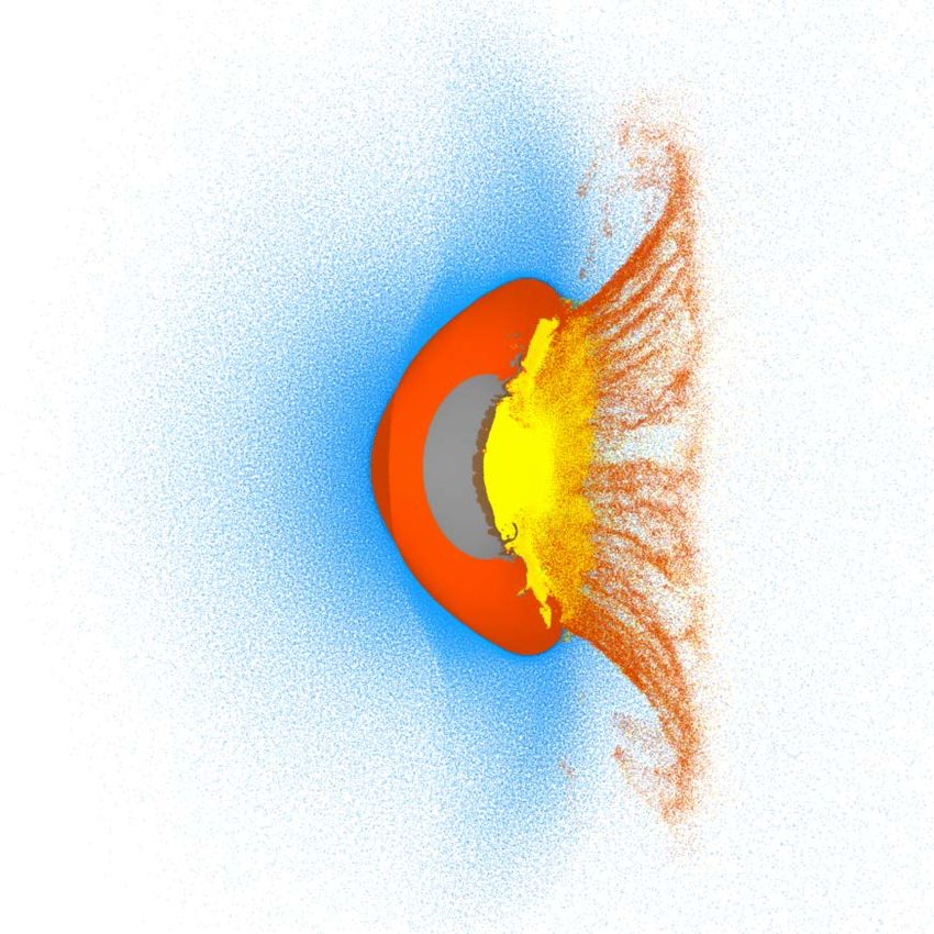
10                                                            Kegerreis et al.

                      b = 0, vc = 1            b = 0.7, vc = 1              b = 0, vc = 3                b = 0.7, vc = 3
                  2
y Position (R⊕)

                  0

           −2
                       vesc

                         −2       0      2        −2       0      2            −2       0      2            −2       0      2
                          x Position (R⊕)          x Position (R⊕)              x Position (R⊕)              x Position (R⊕)
Figure 8. Example positions and velocities of the outermost ‘ground’ particles of the target’s mantle, for the four fiducial
simulations at 0.4, 0.6, 0.2, and 0.2 h after contact, respectively. The colours show the particles’ original longitudes in bins of
10◦ , from 0◦ (pale green) at the point of contact, to 180◦ (red) and −180◦ (blue) at the antipode, here within ±5◦ latitude of
the 0◦ impact plane. The maximum speeds in Fig. 10 are taken from across all snapshot times, whereas only single snapshots
are shown here.
it is the lack of re-impacting fragments that reduces any                 the discrepancies manifest primarily after the initial im-
later erosion.                                                            pact, when debris falls back in and other smaller-scale
   Fig. 7 shows the time evolution for the loss of the                    processes can affect the overall results. Furthermore, re-
different-mass atmospheres. The qualitative evolution                     gions where the atmosphere is only partially lost require
is similar in most cases, especially for the 10−2 and                     many layers of particles to resolve, which is exacerbated
10−2.5 M⊕ atmospheres, and the total loss fraction is                     when additional atmosphere is eroded multiple times af-
systematically lower for the thicker atmospheres. The                     ter the initial shock. While this lack of perfect conver-
drag of the atmosphere as the impactor passes through                     gence is important to note, we can constrain the result-
can reduce the erosion both immediately and by mitigat-                   ing systematic uncertainty for the loss fraction across
ing subsequent oscillations and secondary impacts. For                    the suite of 10−2 M⊕ atmospheres to around 2% in slow
the faster collisions, as before, the behaviour remains                   scenarios and much smaller in more violent cases.
comparatively simple with more immediate erosion and                        In order to further test the dependence of our results
the results are less affected by the atmosphere’s mass in                 on the type of finite-particle issues discussed in relation
terms of timing.                                                          to the slow, head-on collision in the 1st row of Fig. 3,
                                                                          we ran ten duplicate simulations with the target rotated
                        3.3. Convergence and Other Tests
                                                                          to different orientations. Most of the resulting loss frac-
  To study the results of using different particle num-                   tions agree to within a few percent of the mean of 0.47.
bers, we duplicated each of the two slower fiducial simu-                 However, three produced ∼0.07 more fractional erosion
lations and the 10−2 M⊕ -atmosphere fast ones with 106 ,                  and one a remarkable 0.21 less, giving a standard devi-
106.5 , 107.5 , and 108 SPH particles (per Earth mass).                   ation of 0.08. The qualitative evolution appears much
For this initial project, we used 107 particles for the main              the same in all ten cases, but the details of the fall-back
suite to explore this new parameter space. Kegerreis                      and sloshing that follows the initial impact and rebound
et al. (2019) showed that 107 particles are approximately                 (see Fig. 7) can differ significantly in magnitude. This
the minimum number required to resolve all of the ma-                     chaotic behaviour also helps to explain the incomplete
jor processes in sufficient detail. That being said, for the              convergence of the slow, head-on collisions discussed
atmospheric-erosion tests specifically (for thicker atmo-                 above. In contrast, similar rotated re-simulations of fast,
spheres than here), lower particle numbers still yielded                  grazing impacts produced the same results consistently,
results within 10% of the converged value.                                indicating that these issues are restricted to the most
  Fig. 7 shows that the number of particles required for                  sensitive slow, head-on cases. Therefore, we warn that
convergence clearly depends on the scenario in addition                   significant care must be taken when interpreting the re-
to the atmosphere mass. The thicker atmospheres ap-                       sults from one-off simulations of slow, head-on impacts,
pear well converged by only 106.5 particles, as are the                   even at high resolution.
10−2 M⊕ atmospheres for the high-speed scenarios. For                       We ran two additional tests with higher surface tem-
the thinner atmospheres in the slower scenarios, the fi-                  peratures of 1000 and 2000 K on the target in an other-
nal results differ by a few percent even between 107.5                    wise unchanged fast, grazing impact. The resulting loss
and 108 particles. As found by Kegerreis et al. (2019),
Atmospheric Erosion by Giant Impacts 11
Peak Radial Ground Velocity (vesc) Peak Radial Ground Velocity (vesc)
Peak Radial Ground Velocity (vesc) Peak Radial Ground Velocity (vesc)
1.0 1.0 1.0 1.0
Time of Peak Velocity (hours)
Time of Peak Velocity (hours)
b =0 b = 0.7
vc = 1 vc = 1
0.8 0.8 0.8 0.8
0.6 0.6 0.6 0.6
0.4 0.4 0.4 0.4
0.2 0.2 0.2 0.2
0.0 0.0 0.0 0.0
Time of Peak Velocity (hours)
Time of Peak Velocity (hours)
b =0 b 2.5
= 0.7 2.5
vc = 3 vc = 3 0.8 0.8
2.0 2.0
0.6 0.6
1.5 1.5
0.4 0.4
1.0 1.0
0.5 0.2 0.5 0.2
0.0 0.0 0.0 0.0
Figure 9. The maximum outwards radial velocity of the outermost particles of the target’s mantle (top hemispheres) and the
times at which they occur (bottom hemispheres) for the four fiducial simulations, on a Mollweide projection with the point of
contact at (0◦ , 0◦ ) in the centre, as described in Fig. 8. The impacts are symmetric in latitude so only one hemisphere is shown
for each parameter. Note that the top, low-speed pair simulations share the same colour bars that have different limits to those
shared by the bottom, high-speed pair.
fractions were 0.04 and 0.07 higher than the original re- at each location are given in Fig. 9 for the four fiducial
sult of 0.52, respectively. While the warmer atmospheres simulations.
with their greater scale heights are indeed lost slightly The two head-on impacts are symmetric in longitude
more easily, this provides additional confidence that it and show high peak speeds near the impact point and
is only a minor effect. the antipode. For the slower of the two, the target re-
We also re-ran the same fast, grazing impact with a coils following the initial collision to shoot a plume of
target mantle made of basalt (Benz & Asphaug 1999, material back through the point of impact and a slightly
Table II), resulting in a slightly cooler, lower density less dramatic ejection at the antipode, causing the peak
body than the default granite. The resulting loss was velocities in Fig. 9 at those longitudes. Some earlier
only 0.02 greater than the standard case’s 0.52, with ero- erosion around the antipode is also caused by the initial
sion occurring in the same locations at the same times, shock wave, which is the origin of the maximum veloc-
as was also seen in the temperature tests. This sug- ities at most of the other longitudes and latitudes. As
gests that the atmospheric loss is not highly sensitive to shown in Fig. 9, this occurs a bit less than an hour before
mild changes in the target’s material and precise internal the peak recoil.
structure. For the faster head-on collision, the impact is more
destructive and no such bounce-back plume is seen. In-
3.4. Ground Speed stead, almost the entire surface is kicked immediately by
the shock wave to faster than the escape speed, explain-
The one-dimensional estimates of Genda & Abe (2003, ing the near-total erosion of atmosphere plus some lost
hereafter GA03) predict the local atmospheric loss for mantle that was highlighted in Fig. 4. In both head-on
a given vertical ground speed. By defining the ‘ground’ cases, the lower speeds at high latitudes simply reflect
simulation particles as those in the outermost shell of the rotational symmetry (as our planets are not spin-
the target’s mantle, we can track their movement as ning).
shock waves (and the impactor itself) perturb them, as The two grazing collisions show similar behaviour to
illustrated in Fig. 8. We define longitude = 0◦ to be each other with high speeds at positive longitudes, i.e. in
the point of contact with ±180◦ the antipode, and lati- the path of the impactor as it passes through the point of
tude = 0◦ is the impact (z = 0) plane. The maximum contact. The rest of the planet is hit by a shock wave,
outwards radial speed and the time at which it occurs12 Kegerreis et al.
b = 0, vc = 1 0–5◦ b = 0, vc = 3
2.5
Peak Radial Ground Velocity (vesc)
15–20◦
30–45◦
2.0 60–90◦
1.5
1.0
0.5
0.0
−180 −90 0 90 180 −90 0 90 180
Longitude (◦) Longitude (◦)
Figure 10. The maximum outwards radial velocity of the outermost particles of the target’s mantle as a function of longitude
away from the impact point, in separate, similar-area |latitude| bins – effectively showing horizontal slices across Fig. 9 – for
the two head-on fiducial simulations. The dashed lines show the estimated ground speeds at the same latitudes from Inamdar
& Schlichting (2015), based on conserving a point-mass impactor’s momentum in a spherical shock wave.
but not one nearly as strong as in the head-on cases, the peak speed everywhere else and cannot reproduce
and with only a mild peak at the antipode. Unlike the the increase in speed at the antipode. This is unsur-
head-on impacts, the grazing scenarios are not rotation- prising given their assumption that the entire volume
ally symmetric. Higher latitudes are less affected by the of material traversed by the shock is all travelling at
relatively small impactor and show little longitudinal the same speed. In reality and in our simulations, the
variation. shock front moves much faster than the material behind
In the slower grazing collision, the local loss around it. The overprediction near the impact site has little
the impact site happens quickly, but the peak speeds effect on the results as all atmosphere is removed there
everywhere else occur up to an hour later, correspond- regardless, but the low speeds elsewhere lead to signifi-
ing to the initial fall-back of some impactor fragments cant underestimates for the erosion.
and the recoiling oscillation of the planet. In the faster IS15’s model does not include the effects of gravity, the
grazing case, the shock wave quickly produces the peak density profile, rarefaction waves after the shock reaches
speeds across most of the surface, with little significant a surface, and the non-zero size and non-instant momen-
fall-back of fragments. The late times to the positive- tum transfer of the impactor. The internal structure of
longitude side of the impact site are less meaningful since the planet changes dramatically as the large impactor
most of this material is carried away at a roughly con- plunges messily through the mantle; at high speeds, the
stant speed with the surviving impactor, slightly slower impactor can even reach the core of the target well be-
than the impactor’s initial 3 vesc . The peak antipode fore the shock wave has reached the other side. It is
speeds are caused by the violent sloshing of the target possible that with additional modifications such models
as it begins to resettle following the shock. may be made useful, especially for fast, grazing impacts
Fig. 10 shows a subset of the same peak ground where the shock drives the majority of the loss in a sim-
speeds for comparison with those predicted by Inamdar pler manner, though in that case an estimate for the
& Schlichting (2015, hereafter IS15). These are indepen- fraction of the impactor’s momentum that is transferred
dent of the impact parameter so nominally correspond would also be required, dependent on the impact angle,
to head-on collisions. They assume that the impactor’s speed, and planets’ radii.
momentum is transferred at the point of contact and
is conserved with a constant speed of shocked material 3.5. Local and Global Atmospheric Loss
within the propagating spherical shock wave. While this
Now that we have examined the ground speeds across
inevitably overestimates the ground speed close to the
the planet for the fiducial impacts and introduced 1D
point-mass impact, it also significantly underestimates
and analytical estimates for comparison, we show inAtmospheric Erosion by Giant Impacts 13
1.0 1.0
Atmosphere Mass Loss Fraction
Atmosphere Mass Loss Fraction
b =0 b = 0.7
vc = 1 vc = 1
0.8 0.8
0.6 0.6
0.4 0.4
0.2 0.2
X = 0.15 X = 0.08
XGA03 = 0.24 X0.0
GA03 = 0.13 0.0
1.0 1.0
Atmosphere Mass Loss Fraction
Atmosphere Mass Loss Fraction
b =0 b = 0.7
vc = 3 vc = 3
0.8 0.8
0.6 0.6
0.4 0.4
0.2 0.2
X = 1.00 X = 0.35
XGA03 = 1.00 X0.0
GA03 = 0.38 0.0
Figure 11. The loss fraction of local atmosphere (top hemispheres) for the four fiducial simulations, on a Mollweide projection
as in Fig. 9. The bottom hemispheres show the corresponding loss estimates from Genda & Abe (2003, GA03) using the peak
ground speeds from our study that are shown in Fig. 9. The annotations give the total loss, X, from the simulations globally
for comparison with the total GA03 estimates.
Fig. 11 the local atmospheric mass loss in each region which, if used instead, produce slightly different qualita-
for the four fiducial impacts. tive results but very similar values for the total erosion.
The loss fractions broadly follow the distributions of Another important issue is the large size of the im-
peak ground speeds in Fig. 9, and the GA03 results pactor and its complicated interaction with the target,
based on our peak speeds also match well the simu- compared with a simple point-mass explosion that would
lated loss in many places. Encouragingly, this implies better produce loss just from ground shocks. Significant
that their 1D calculations and our SPH simulations re- amounts of material can thus be ejected directly by the
produce similar results for a ground shock wave eroding impactor ploughing through the atmosphere and man-
the atmosphere above it once it arrives at the surface. tle, especially in grazing impacts.
This is not always the case for the more complicated Finally, there are the underlying assumptions made
scenarios we are dealing with here. Perhaps the most and discussed by GA03, such as their use of an ideal
significant reason is that for these estimates we have gas EoS and ignoring lateral motion of the atmosphere,
taken a single value for the peak ground speed at each lo- both of which are likely to be more valid in their tar-
cation, whereas in reality the atmosphere can be ejected geted regime of even thinner atmospheres. However, the
at many points in time – as was shown in Fig. 9. We fact that our simulations agree with theirs in many cases
also cannot fix this simplification by applying GA03’s suggests that these simplifications are often not too im-
estimates at, for example, all local-in-time maximum portant.
ground speeds, simply because the atmosphere must still The overall results for the suite are presented in
be present above the ground for a shock to remove it. Fig. 12, showing how the fraction of lost atmosphere
After the initial impact, some parts of the atmosphere varies with atmosphere mass, impact parameter, and
could survive relatively undisturbed and be removed by speed. We find that, unsurprisingly, more atmosphere
subsequent shocks. However, other parts could be par- is usually lost from smaller atmospheres, more-head-on
tially shocked away to fall back down at a later time, collisions, and higher speeds. However, for slower col-
which may or may not coincide with later shocks. Thus, lisions, the loss is not a monotonic function of the im-
the assumption of a single ground speed could either pact parameter, and a head-on collision does not cause
over- or underestimate the actual local loss. We also the most erosion. By hitting slightly off-centre, the
used the radial ground speeds rather than the total, impactor can both deliver a strong shock through the
planet while also encountering and eroding more atmo-14 Kegerreis et al.
1.0
vc = 1
vc = 2
Atmosphere Mass Loss Fraction
vc = 3
0.8
0.6 b = 0, vc = 1
b = 0.7, vc = 1
b = 0, vc = 3
0.4 b = 0.7, vc = 3
0.2
b=0
b = 0.7
0.0
10−2 10−1 0.0 0.2 0.4 0.6 0.8 0 2 4 6 8
Atmosphere Mass (M⊕) Impact Parameter Speed at Contact (vesc)
Figure 12. The lost mass fraction of the atmosphere for different: (left) atmosphere masses, in each of the fiducial impact
scenarios; (middle) impact parameters, for three different speeds; and (right) speeds at contact, for each fiducial impact param-
eter; all with ∼107 particles. The error bars in the left panel show the approximate, conservative uncertainty due to incomplete
numerical convergence, which becomes significant for the lowest atmosphere mass. The circles show the corresponding Genda &
Abe (2003) estimates based on the peak ground speeds. For the head-on collisions, the crosses show the Inamdar & Schlichting
(2015) estimates based solely on the impactor’s mass and speed relative to the target (their Fig. 4).
sphere directly. Although more-grazing impacts can di- 100
rectly remove even more local material, they fail to de-
posit enough energy into the shock to erode as much
Atmosphere Mass Loss Fraction
atmosphere on the far side.
Apart from this, by following the same ground-speed
analysis as for the fiducial impacts, the GA03 estimates b
0
continue to reproduce the results well in most cases. As
0.1
indicated by the ground speeds in Fig. 10, the estimates
0.2
from IS15 predict far less loss than most head-on colli-
0.3
sions.
10−1 0.4
Bearing in mind that the results for the smallest at-
0.5
mospheres are not fully converged numerically, we find
0.6
a relatively mild dependence on the initial atmosphere
0.7
mass, partly depending on the specific scenario. This 0.8
is supported by the good agreement of the GA03 es- 0.9
timates, which assumed a much thinner atmosphere
than ours along the lines of the Earth’s present-day, 105 106 107 108
∼10−6 M⊕ atmosphere. Specific Impact Energy, Q (J kg−1)
In spite of the complicated details, including signif-
icant non-monotonic dependence on the angle at low Figure 13. The lost mass fraction of the atmosphere for
speeds, we find that a single parameter can be used to es- all the simulation scenarios as a function of their modified
specific impact energy (Eqn. 1), coloured by their impact
timate the erosion from any scenario. Fig. 13 shows the
parameter. The black line shows our power-law fit (Eqn. 2).
fraction of atmosphere lost, X, as a function of the mod- The lower black square corresponds to the canonical Moon-
ified specific impact energy, based on the specific energy forming impact (Canup & Asphaug 2001), and the other
used by Leinhardt & Stewart (2012) to predict disrup- two to more recent, higher energy scenarios (Ćuk & Stewart
tion. We find that an additional factor of (1−b)2 (1+2b) 2012; Lock et al. 2018). These results are also presented
broadly accounts for the variation across the full range numerically in Table 1.
of head-on to highly grazing collisions:
where vc is here the SI value not normalised by the es-
cape speed, and µr ≡ Mi Mt /Mtot is the reduced mass.
Q = (1 − b)2 (1 + 2b) 12 µr vc2 / Mtot , (1) The added term loosely accounts for the fractional vol-Atmospheric Erosion by Giant Impacts 15
ume of the two bodies that interacts: the volume of the where more atmosphere is lost. Low-speed head-on col-
target cap above the lowest point of the impactor at lisions are particularly chaotic even at high resolution,
contact, plus the volume of the impactor cap below the making convergence harder to achieve. We conclude
highest point of the target, divided by the total volume, that bespoke convergence tests continue to be crucial
is 41 [(Rt + Ri )3 /(Rt3 + Ri3 )](1 − b)2 (1 + 2b) (see Appx. B). for any project using planetary SPH simulations. That
In reality, this is not the exact volume of material that being said, our results provide the rough rule of thumb
actually interacts, especially for low-speed collisions or that about ten layers of SPH particles are required to
smaller impactors. Nonetheless, we find empirically that model the evolution of an atmosphere in these types of
it allows a simple power-law fit for the loss fraction to scenarios.
be made in this regime, as shown in Fig. 13: By tracking the ground movement throughout the
0.67 simulations, we compared these 3D results with Inam-
X ≈ 7.72×10⁻⁶ Q / J kg−1 , (2) dar & Schlichting (2015, IS15)’s analytical estimates for
the propagation of shocks from a giant impact, Genda
capped at one for total erosion. Note that the effects
& Abe (2003, GA03)’s 1D models for local shock-driven
of changing the impact angle may have an additional
erosion, and IS15’s combined predictions for the global
dependence on the impactor’s mass and radius, so from
loss in a given scenario. IS15’s ground velocities signif-
this initial study alone we can only be certain of this
icantly underestimate the maximum ground speeds in
scaling law’s applicability to bodies of this size. Its po-
head-on impacts owing to the dramatic deformation of
tential extrapolation to wider scenarios will be examined
the planet and violent post-impact oscillations. For the
in a future study (Kegerreis et al., in prep).
same reasons, their global predictions underestimate the
4. CONCLUSIONS total loss. Using our simulated ground speeds, GA03’s
estimates match the localised loss fractions well in most
We have presented 3D simulations of giant impacts
cases, especially when the direct encounter of the im-
onto terrestrial planets with thin atmospheres. We ex-
pactor with the atmosphere is not too important.
plored a wide variety of speeds and impact angles, as
In the context of the Earth and the canonical Moon-
well as a small range of atmosphere masses, and found
forming impact, only around 10% of the atmosphere
a simple scaling law to estimate the fraction of atmo-
would have been lost from the immediate effects of the
sphere lost in this regime of approximately Earth-mass
collision. This suggests that the canonical impact it-
targets and Mars-mass impactors.
self cannot single-handedly explain the discrepancies be-
Several different processes can dominate the atmo-
tween the volatile abundances of the Earth and chon-
spheric loss in different scenarios, depending on, for ex-
drites by eroding the early atmosphere, compared with
ample, whether the impactor can deliver a strong shock
alternative, more-violent Moon-forming scenarios. How-
wave to remove atmosphere on the far side, or whether
ever, the caveat of ‘immediate’ erosion is important,
impactor fragments fall back after the initial collision.
because we have here only considered the direct, dy-
The interplay of these and other processes affects the
namical consequences of a giant impact. As examined
total fraction of eroded atmosphere, the local distribu-
by Biersteker & Schlichting (2019), the thermal effects
tion of where atmosphere is lost, and the time at which
of a giant impact heating the planet might erode com-
it is removed.
parable atmosphere to that ejected by shocks, though
For head-on collisions, there is a rapid change with
the volatile loss may not be that efficient even from a
increasing impact speed from very little erosion to total
hot post-impact disk (Nakajima & Stevenson 2018). In
loss. However, for grazing impacts with changing speed
addition, we took the simple approach here of defining
– or for fixed speeds with changing impact angle – there
‘lost’ atmosphere by particles that become gravitation-
is a much more gradual transition of partial erosion that
ally unbound, ignoring the fact that significant material
also displays complex, non-monotonic behaviour at low-
can remain bound and still be ejected far away from the
to-medium impact parameters.
planet. In a real planetary system, whether by interac-
We find that numerical convergence can require many
tion with the solar wind or by leaving the target’s Hill
more than 106 SPH particles, with a strong dependence
sphere of gravitational influence, much of the eroded-
on the specific impact scenario and the measurement
but-bound atmosphere could still be lost. As a separate
in question, consistently with Kegerreis et al. (2019).
point, Genda & Abe (2005) showed that the presence
The majority of our simulations used ∼107 particles,
of an ocean can significantly enhance atmospheric loss,
which agree with simulations using 107.5 and 108 on
such that in the canonical Moon-forming scenario, closer
the fraction of atmosphere lost to within a few per-
to half the atmosphere could be immediately removed.
cent, with complete convergence in high-speed scenarios16 Kegerreis et al.
Their models combined with our results could be used ACKNOWLEDGMENTS
to estimate the amount of an ocean that would be re-
moved in different scenarios, to constrain the extent of We thank the anonymous reviewer for their con-
fractionation between volatiles. Future simulation stud- structive and insightful comments. The research in
ies could potentially resolve an ocean directly and test this paper made use of the SWIFT open-source sim-
such erosion in more realistic detail. ulation code (www.swiftsim.com, Schaller et al. 2018)
The details of atmospheric erosion by giant impacts version 0.8.5. This work was supported by the Sci-
are complicated. These simulations provide a simple ence and Technology Facilities Council (STFC) grant
scaling law in this regime and form a starting point ST/P000541/1, and used the DiRAC Data Centric
from which to explore the vast parameter space in detail. system at Durham University, operated by the Insti-
Promising targets for future study include: investiga- tute for Computational Cosmology on behalf of the
tions of different impactor and target masses; extensions STFC DiRAC HPC Facility (www.dirac.ac.uk). This
to both more massive and even thinner atmospheres; the equipment was funded by BIS National E-infrastructure
inclusion of an atmosphere on the impactor as well as capital grant ST/K00042X/1, STFC capital grants
the target; and testing the dependence on the planets’ ST/H008519/1 and ST/K00087X/1, STFC DiRAC Op-
materials, internal structures, and rotation rates. This erations grant ST/K003267/1 and Durham University.
way, robust scaling laws could be built up to cover the DiRAC is part of the National E-Infrastructure. JAK
full range of relevant scenarios in both our solar sys- is supported by the ICC PhD Scholarships Fund and
tem and exoplanet systems for the loss and delivery of STFC grants ST/N001494/1 and ST/T002565/1. RJM
volatiles by giant impacts. is supported by the Royal Society.
Software: SWIFT (www.swiftsim.com, Kegerreis
et al. (2019), Schaller et al. (2016), version 0.8.5);
SEAGen (pypi.org/project/seagen/).
APPENDIX
A. IMPACT INITIAL CONDITIONS is in the x direction.
For each scenario, we choose the impact parameter, −1
v2
b = sin(β), and the speed, vc , that the impactor would 2
a= − c (A4)
reach at first contact with the target, as illustrated in rc µ
s
Fig. 1. The distance between the body centres and the 2 1
y position at contact are v= µ − (A5)
r a
yc vc
y= , (A6)
rc = Ri + Rt (A1) v
yc = b rc . (A2) where a is the semi-major axis, which is negative for
hyperbolic orbits, and vc is the speed at contact.
The velocity at infinity, In order to rotate the coordinate system such that, at
contact, the velocity will be in the x direction (a purely
p aesthetic choice), we first find the periapsis, rp , and then
vinf = vc2 − 2µ/rc , (A3) the eccentricity, e. Taking the vis-viva equation at peri-
apsis and using Eqn. A6 to eliminate the speed gives
is zero for a parabolic orbit when vc = vesc , where
av 2 y 2
µ = G(Mt + Mi ) is the standard gravitational param- rp2 − a rp + 2µc c
=0 (A7)
eter and vesc is the two-body escape speed. Note that q
2av 2 y 2
for targets with atmospheres, we account for the mass a ± a2 − µc c
rp = (A8)
of the atmosphere but ignore its thickness. 2
For elliptical or hyperbolic orbits, the speed and y po- e = 1 − rp /a , (A9)
sition at any earlier time can be calculated using the
vis-viva equation and conservation of angular momen- which allows calculation of the true anomaly (in this
tum, where y is in the rotated reference frame where v case its complement, θ) and the angle of the velocityYou can also read