Comparison of source apportionment approaches and analysis of non-linearity in a real case model application - GMD
←
→
Page content transcription
If your browser does not render page correctly, please read the page content below
Geosci. Model Dev., 14, 4731–4750, 2021
https://doi.org/10.5194/gmd-14-4731-2021
© Author(s) 2021. This work is distributed under
the Creative Commons Attribution 4.0 License.

Comparison of source apportionment approaches and analysis of
non-linearity in a real case model application
Claudio A. Belis1 , Guido Pirovano2 , Maria Gabriella Villani3 , Giuseppe Calori4 , Nicola Pepe4 , and
Jean Philippe Putaud1
1 European Commission, Joint Research Centre, via Fermi 2748, 21027 Ispra (VA), Italy
2 RSE Spa, via Rubattino 54, 20134 Milan (MI), Italy
3 ENEA Laboratory of Atmospheric Pollution, via Fermi 2748, 21027 Ispra (VA), Italy
4 ARIANET s.r.l. via Gilino 9, 20128 Milan (MI), Italy

Correspondence: Claudio A. Belis (claudio.belis@ec.europa.eu)

Received: 5 December 2020 – Discussion started: 16 February 2021
Revised: 19 May 2021 – Accepted: 22 June 2021 – Published: 29 July 2021

Abstract. The response of particulate matter (PM) concen-          ever, in many situations the non-linearity in PM10 annual av-
trations to emission reductions was analysed by assessing the      erage source allocation was negligible, and the TS and BF
results obtained with two different source apportionment ap-       approaches provided comparable results. PM mass concen-
proaches. The brute force (BF) method source impacts, com-         trations attributed to the same sources by TS and BF were
puted at various emission reduction levels using two chem-         highly comparable in terms of spatial patterns and quantifi-
ical transport models (CAMx and FARM), were compared               cation of the source allocation for industry, transport and res-
with the contributions obtained with the tagged species (TS)       idential combustion. The conclusions obtained in this study
approach (CAMx with the PSAT module). The study fo-                for PM10 are also applicable to PM2.5 .
cused on the main sources of secondary inorganic aerosol
precursors in the Po Valley (northern Italy): agriculture, road
transport, industry and residential combustion. The interac-
tion terms between different sources obtained from a factor        1   Introduction
decomposition analysis were used as indicators of non-linear
PM10 concentration responses to individual source emission         Air pollution is the main environmental cause of premature
reductions. Moreover, such interaction terms were analysed         death. Ambient air pollution caused 4.2 million deaths world-
in light of the free ammonia / total nitrate gas ratio to deter-   wide in 2016, contributing together with indoor pollution
mine the relationships between the chemical regime and the         to 7.6 % of all deaths (WHO, 2018). Air pollution adverse
non-linearity at selected sites. The impacts of the different      health effects mainly occur as respiratory and cardiovascu-
sources were not proportional to the emission reductions, and      lar diseases (WHO, 2016; EEA 2019). A key element for the
such non-linearity was most relevant for 100 % emission re-        design of effective air quality control strategies is the knowl-
duction levels compared with smaller reduction levels (50 %        edge of the role of different emission sources in determin-
and 20 %). Such differences between emission reduction lev-        ing the ambient concentrations. This is usually referred to as
els were connected to the extent to which they modify the          source apportionment (SA) and involves the quantification of
chemical regime in the base case. Non-linearity was mainly         the influence of different human activities (e.g. transport, do-
associated with agriculture and the interaction of this source     mestic heating, industry, agriculture) and geographical areas
with road transport and, to a lesser extent, with industry. Ac-    (e.g. local, urban, metropolitan areas, countries) to air pollu-
tually, the mass concentrations of PM10 allocated to agri-         tion at a given location.
culture by the TS and BF approaches were significantly dif-           SA modelling studies involving secondary inorganic pol-
ferent when a 100 % emission reduction was applied. How-           lutants are generally based on chemistry transport models
                                                                   (Mircea et al., 2020). Two different SA approaches are com-

Published by Copernicus Publications on behalf of the European Geosciences Union.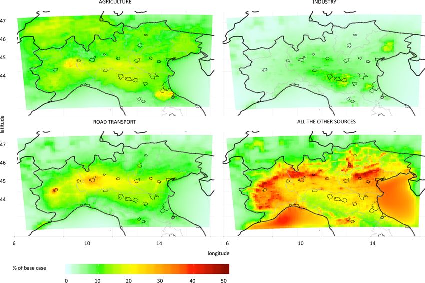
4732                     C. A. Belis et al.: Comparison of source apportionment approaches and analysis of non-linearity

monly used to allocate the mass of pollutants to the different     counting, chemical regime limited by one precursor, com-
sources by means of chemical transport models.                     petition between precursors, thermodynamic equilibrium be-
  – “Tagged species” (TS) quantifies the contribution of           tween the secondary pollutant and its precursors, and com-
    emission sources to the concentration of one pollutant         pensation. A detailed explanation of each of them is provided
    at one given location by implementing algorithms to            in Appendix A.
    trace reactive tracers. SA studies based on tagging meth-         In the analysis of a theoretical example with three sources
    ods have been carried out at both European scale (e.g.         (agriculture, industry and residential), Clappier et al. (2017)
    Karamchandani et al., 2017; Manders et al., 2017) and          observed that strong non-linearity is associated with sec-
    urban scale (e.g. Pepe et al., 2019; Pültz et al., 2019).      ondary inorganic aerosol (SIA, ammonium nitrate and am-
                                                                   monium sulfate) formation. However, this secondary aerosol
  – Brute force (BF or emission reduction impact) is a sen-        may behave linearly or non-linearly depending on the cir-
    sitivity analysis technique which estimates the change         cumstances, for instance, the intensity of the emission re-
    in pollutant concentration (impact) that results from          duction, which imposes the need to quantify it for different
    a change in one or more emission sources. Sensitiv-            emission reduction levels (ERLs) (see Sect. 3.2). Thunis et al.
    ity analysis techniques have been used to estimate the         (2015) showed that for yearly average relationships between
    impact of different sources on pollution levels (e.g.          emission and concentration changes, linearity is often a real-
    Kiesewetter et al., 2015; Thunis et al., 2016; Van Din-        istic assumption and, consequently, TS and BF methods are
    genen et al., 2018).                                           expected to provide comparable results, as reported by Belis
Even though these approaches are often considered as two           et al. (2020a). The abovementioned considerations suggest
alternative SA methods, they actually pursue different objec-      the need to monitor whether non-linearity is significant for a
tives: TS aims to account for the mass transferred from the        given study area and time window.
sources to the receptor in a specific area and time window,           The objective of this study is to identify and quantify the
while BF is a sensitivity analysis technique used to estimate      factors leading to non-linear response of PM concentrations
the response of the system to changes in emissions. For a de-      to source emission reductions in a real-world situation with
tailed discussion, refer to Belis et al. (2020a), Mircea et al.    significant PM concentrations. To that end, the influence on
(2020), and Thunis et al. (2019).                                  PM10 concentration of various sources with different chemi-
   Clappier et al. (2017) applied the concept of factor de-        cal profiles was calculated using both the BF approach with
composition developed by Stein and Alpert (1993) to inves-         two different chemical transport models (CAMx and FARM)
tigate the differences between TS and BF using a theoreti-         and the TS approach using one of these chemical-transport
cal example involving three sources. According to these au-        models (CAMx).
thors, the change in concentration of a given pollutant due           The results of the simulations were then used to
to the change in the emissions of three sources A, B and C
                                                                       – compare TS contributions with BF impacts,
(1CABC ) can be described as follows:
1CABC = 1CA +1CB +1CC +ĉAB +ĉAC +ĉBC +ĉABC , (1)                   – analyse the geographical patterns,
where 1CA , 1CB and 1CC are the variations of concentra-               – compute interaction terms (of the Stein and Alpert alge-
tion of the studied pollutant due to the reduction in the single         braic expression) for the studied sources, and
sources A, B and C, respectively, and those coming from the
interactions between these sources denoted by the terms ĉAB ,         – compare the behaviour of various areas (urban, rural,
ĉAC , ĉBC and ĉABC (see Appendix A for details). The inter-           etc.) with different chemical regimes.
action terms (ĉ) have the same units as the source impacts.
                                                                   In this study, the focus is on the non-linearity associated with
   In the TS approach, the sum of the contributions of the var-
                                                                   SIA formation, with particular reference to ammonium ni-
ious sources always matches the total pollutant concentration
                                                                   trate (NH4 NO3 ) and ammonium sulfate ((NH4 )2 SO4 ). The
by design (Mpoll = MA + MB + MC ), while this may be not
                                                                   possible non-linear behaviour of any other PM component
the case for the BF approach (1CABC 6 = 1CA +1CB +1CC )
                                                                   (e.g. organics) is beyond the scope of this exercise.
under certain circumstances (Belis et al., 2020a). The inter-
action terms in Eq. (1) measure the consistency between the
sum of single emission sources with respect to the contem-         2    Materials and methods
porary reduction in more than one source in BF, for three
sources 1CABC −(1CA +1CB +1CC ), which is an indica-               The Po Valley was selected for this study because of its high
tor of the non-linearity in the response of the pollutant con-     levels of particulate matter due to the high emissions of pri-
centration to single-source reductions (impacts).                  mary pollutants and precursors of SIA, whose high concen-
   There are different situations that may contribute to gener-    trations are also favoured by the stagnation of air masses dur-
ating non-linear responses when secondary pollutants’ pre-         ing the coldest months of the year (Belis et al., 2011; Larsen
cursors are emitted by different sources. They are double          et al., 2012).

Geosci. Model Dev., 14, 4731–4750, 2021                                             https://doi.org/10.5194/gmd-14-4731-2021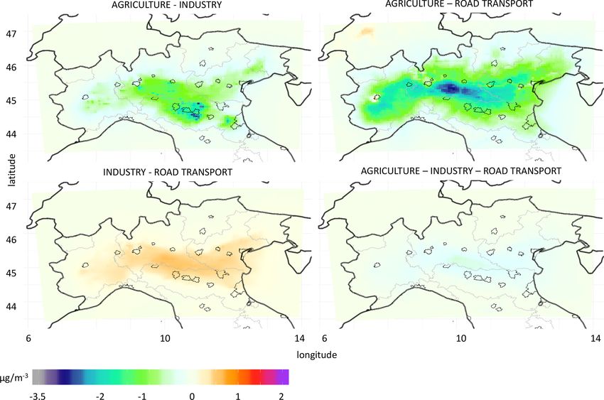
C. A. Belis et al.: Comparison of source apportionment approaches and analysis of non-linearity                            4733

   The air quality simulations were performed with the             computed using the O’Brien scheme (O’Brien, 1970) but
CAMx (ENVIRON, 2016) and FARM (ARIANET, 2019)                      adopting two different minimum Kv values for rural and ur-
chemical transport models (CTMs). Both are open-source             ban areas so as to consider heat island phenomena and in-
modelling systems for multi-scale integrated assessment of         creased roughness of built areas.
gaseous and particulate air pollution. Thanks to their variable       FARM simulations were performed using the SAPRC-99
spatial resolution, they are used for urban- to regional-scale     gas-phase chemical mechanism (Carter, 2000) and a three-
applications and, simulating the atmospheric chemical reac-        mode aerosol scheme (Binkowski and Roselle, 2003) includ-
tions of the emitted precursors, they allow reconstruction of      ing microphysics, ISORROPIA for thermodynamic equilib-
the formation of most of the secondary compounds, includ-          rium of inorganic species and SORGAM (Schell et al., 2001)
ing the constituents of particulate matter. CAMx is widely         for secondary organic aerosol formation. Meteorological in-
used to assess the influence of pollution sources on air quality   put from WRF was complemented by Kv computed using
in a particular domain. The PM source apportionment tech-          Lange (1989) parameterisation.
nology (PSAT; Yarwood et al., 2004) implemented in CAMx               Emissions were derived from inventory data
offers the choice between several SA approaches, which al-         at     three    different   levels:     European     Monitor-
lows users to easily compare e.g. TS versus BF methods for         ing     and    Evaluation      Programme       data   (EMEP,
the estimation of source contributions to pollutant concentra-     https://www.ceip.at/webdab-emission-database/
tions using the same model. In addition, the application of the    emissions-as-used-in-emep-models,            last      access:
BF method with FARM made it possible to show the struc-            13 July 2021) available over a regular grid of
tural behaviours that are less dependent on the specific model     50 × 50 km2 and ISPRA Italian national inventory data
formulation and consequently to obtain results of more gen-        (http://www.sinanet.isprambiente.it/it/sia-ispra/inventaria/
eral value.                                                        disaggregazione-dellinventario-nazionale-2015/view, last
   The application of such CTMs required the implementa-           access: 13 July 2021), which provide a disaggregation by
tion of a comprehensive modelling system (e.g. Pepe et al.,        province. Moreover, regional inventory data based on the
2019), including specific tools aiming at creating the three       INEMAR methodology (INEMAR – ARPA Lombardia,
main input categories: meteorological fields, emissions and        2015) provided detailed emission data at municipality level
boundary conditions.                                               for the four administrative regions of Lombardy, Piedmont,
   Both modelling systems were applied for the reference           Veneto and Emilia-Romagna.
year 2010 over northern Italy (Figs. S1 and S2 in the Sup-            Each emission inventory was processed to obtain the
plement) considering a computational domain that covers a          hourly time pattern of the emissions. For the CAMx simu-
580 × 400 km2 region, with a 5 km grid step. For the meteo-        lations this was accomplished using the Sparse Matrix Op-
rological model WRF (Skamarock et al., 2008) three nested          erator for Kernel Emissions model (SMOKE v3.5) (UNC,
grids were used, the largest one covering Europe and north-        2013). Temporal disaggregation was based on monthly, daily
ern Africa and the innermost one corresponding to Italy and        and hourly profiles deduced by CHIMERE (INERIS, 2006)
the Po Valley, respectively. The three meteorological do-          and EMEP models from the Institute of Energy Economics
mains have 45, 15, and 5 km grid resolution. For CTMs only         and the Rational Use of Energy (IER) project named GENE-
the innermost WRF nested grid was used. Both CTMs were             MIS (Pernigotti et al., 2013). Similar emission inventory pro-
set up using the same input meteorological data and horizon-       cessing was performed for FARM using the Emission Man-
tal grid structure of WRF. The CTM vertical grid was de-           ager pre-processing system (ARIA Technologies and ARI-
fined by collapsing the 27 vertical layers used by WRF into        ANET, 2013).
14 layers while keeping identical the layers up to 1 km above         Initial and boundary conditions were taken from a par-
ground level; in particular, the first layer thickness was up      ent CAMx simulation covering the whole of Italy and driven
to about 25 m from the ground like the corresponding WRF           by the MACC-II system (https://cordis.europa.eu/project/id/
layer.                                                             283576, last access: 14 July 2021) that provides 3D global
   In CAMx, homogenous gas-phase reactions of nitrogen             concentration fields.
compounds and organic species were reproduced through                 The CAMx modelling system was applied with the pre-
the CB05 mechanism (Yarwood et al., 2005). The aerosol             viously described setup in order to perform a TS run (with
scheme was based on two static modes (coarse and fine).            PSAT) and three sets of BF runs with 100 %, 50 % and 20 %
Secondary inorganic compound evolution was described               emission reduction levels (ERLs), while FARM was used to
by the thermodynamic model ISORROPIA (Nenes et al.,                produce two sets of BF runs with 50 % and 20 % ERLs. Due
1998), while SOAP (ENVIRON, 2011) was used to de-                  to the high number of runs needed to apply the Stein and
scribe secondary organic aerosol formation. Meteorological         Alpert decomposition, only a few sources were selected (Ta-
input data were provided by WRF and were completed by              ble 1). Originally, the study focused on the same system of
OMI satellite data (https://nasatoms.gsfc.nasa.gov, last ac-       three sources (AGR, IND, RES) as the study by Clappier et
cess: 13 July 2021), including ozone vertical content and          al. (2017). However, due to the small non-linearity associ-
aerosol turbidity. Vertical turbulence coefficients (Kv) were      ated with RES, the focus was then shifted to a ternary sys-

https://doi.org/10.5194/gmd-14-4731-2021                                             Geosci. Model Dev., 14, 4731–4750, 2021
4734 C. A. Belis et al.: Comparison of source apportionment approaches and analysis of non-linearity
Table 1. Macro-sectors according to the EEA SNAP classification for emission inventories used to define air pollution sources in this study.
Source: SNAP macro-sector SNAP macro-sector number Abbreviation used in this study
Energy industry 1 OTHER
Residential and commercial/institutional combustion 2 RES
Industry (combustion and processes) 3 and 4 IND
Fugitive emissions from fuels 5 OTHER
Product use including solvents 6 OTHER
Road transport 7 TRA
Non-road transport 8 OTHER
Waste treatment 9 OTHER
Agriculture 10 AGR
tem including AGR, TRA and IND. In total, 41 runs were between different ERLs is discussed in Sect. 3.2. To facil-
performed, keeping all inputs as the base case (BC), except itate the comparison between different models, impacts are
for emissions that were modified according to the scheme re- expressed as a percentage of the base case in these figures.
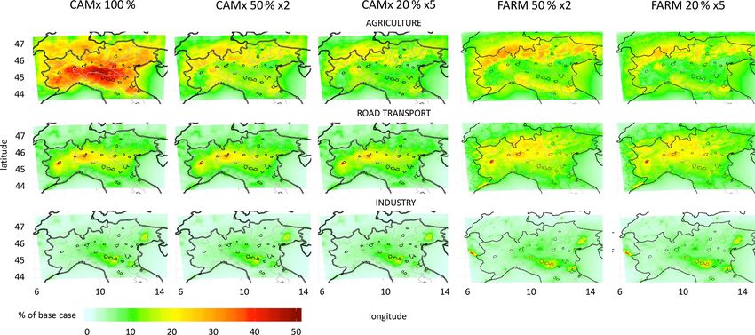
ported in Table 2. In Fig. 2, the highest impacts are those of AGR followed by
In this study, the interactions between sources AGR, TRA TRA and IND. The outputs resulting from CAMx and FARM
and IND are mainly analysed. Additional runs were executed for 50 % and 20 % ERLs present similar levels and geograph-
using FARM at 50 % and 20 % ERLs to test also the impacts ical patterns. Most of the highest impacts of AGR at 100 %
and interactions of RES with the previous ones. ERL are observed in or near the areas of high NH3 emis-
sions (Fig. S4 in the Supplement), in which TS also points
to high contributions of this source (Fig. 1). However, in
3 Results and discussion these areas the BF impacts are nearly twice the TS contri-
butions reported in Fig. 1 (see also Fig. 3, top left). Such
3.1 Comparison between source apportionment TS high levels could be attributed to a near-double-counting ef-
and BF approaches fect which is dominant only at this ERL because the effect
of a limited chemical regime cannot be observed at 100 %
The yearly average PM10 concentrations in the CAMx and reduction (see Appendix A Sect. A2.2). At 50 % and 20 %
FARM base case runs are shown in Figs. S1 and S2. Fig- ERLs the impacts are lower than 100 % ERL, because of
ure 1 shows the relative contributions of the modelled PM10 the limited regime, and the highest ones are located in the
sources using the TS approach (CAMx-PSAT). The contri- mountainous areas (Alps and Apennines). Such a pattern is
butions of AGR are distributed across the entire Po Val- likely due to the low emissions of the SIA precursors (NH3 ,
ley, with maximum levels in the centre and hotspots to the NOx and SO2 ) (Fig. S4) and the modest base case PM10 con-
NW and SE. The IND contributions are highest to the south, centrations in these areas. For IND and TRA, the geograph-
SE and NE of the study area. The TRA contributions to ical patterns of BF are comparable to those of TS (Figs. 1
PM10 are highest in the main urban areas, in particular Mi- and 3 left) and do not vary significantly between the differ-
lan and Turin, and along the main highways (e.g. A4 Turin– ent ERLs, as discussed in Sect. 3.2. The only remark is that
Venice). The highest contributions of all the other remaining FARM presents higher TRA impacts in the subalpine areas
sources (OTHER) are observed in the pre-Alpine area and in compared to CAMx, irrespective of the SA approach used.
the Alpine valleys (including some areas in the Apennines), As shown in Fig. 3, the single grid cell annual averages
where the average PM10 levels are lower than the Po Val- of BF impacts on PM10 by IND and TRA plotted versus the
ley (Figs. S1 and S2) and RES is an important source (see TS contributions are arranged on a line close to the identity,
below). indicating that BF and TS approaches lead to similar results
The annual average impacts of AGR, TRA and IND on for these two sources. A similar behaviour is observed in all
PM10 derived by the BF approach with CAMx and FARM the ERLs even though the BF impacts estimated with FARM
for different emission reduction levels (ERLs) are shown in present a higher dispersion than those obtained with CAMx.
Fig. 2, while those of RES are shown in Fig. S3 in the Sup- Such a closer relationship between TS (CAMx-PSAT) and
plement. In a linear situation the impacts allocated to each CAMx BF results is likely a consequence of both being re-
source decrease proportionally to the intensity of the emis- sults of the same model. By contrast, the impacts of AGR on
sion reduction (1C100 % = 21C50 % = 51C20 % ). For that PM10 at 100 % ERL are more than twice the TS contributions
reason, the impacts at 100 % ERL can be compared directly in most grid cells, which is due to the much greater AGR BF
with TS contributions, while those of 50 % and 20 % must impacts on sulfate and nitrate than TS contributions at this
be multiplied by factors 2 and 5, respectively. The linearity ERL (Figs. S5 and S6 in the Supplement, respectively). Such
Geosci. Model Dev., 14, 4731–4750, 2021 https://doi.org/10.5194/gmd-14-4731-2021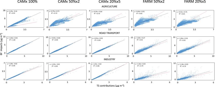
C. A. Belis et al.: Comparison of source apportionment approaches and analysis of non-linearity                                      4735

Table 2. Sets of simulations performed in this study to compute the factor decomposition (Stein and Alpert, 1993). Every set is named after
the used CTM and ERL.

                                                                        Simulation set
                     Reduced sources     CAMx 100 %       CAMx 50 %       CAMx 20 %       FARM 50 %       FARM20 %
                     No reduction                      Base case CAMx                          Base case FARM
                     AGR                       x                x              x               x               x
                     IND                       x                x              x               x               x
                     TRA                       x                x              x               x               x
                     RES                                                                       x               x
                     AGR–IND                   x                x              x               x               x
                     AGR–TRA                   x                x              x                               x
                     IND–TRA                   x                x              x               x               x
                     RES–IND                                                                   x               x
                     RES–TRA                                                                   x
                     RES–AGR                                                                   x
                     AGR–IND–TRA               x                x              x                               x
                     RES–IND–TRA                                                               x               x

Figure 1. Annual contributions of the PM10 sources over the Po Valley area according to the tagged species (TS) approach as computed by
CAMx-PSAT. The grey lines indicate the boundaries of the regions and the polygons represent the municipal areas of the main cities.

https://doi.org/10.5194/gmd-14-4731-2021                                                   Geosci. Model Dev., 14, 4731–4750, 2021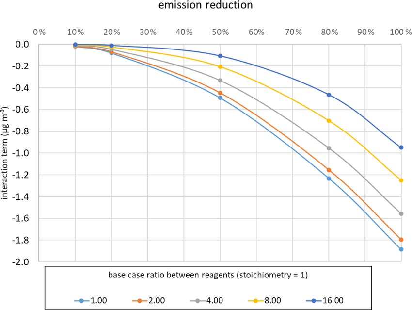
4736                    C. A. Belis et al.: Comparison of source apportionment approaches and analysis of non-linearity

Figure 2. Annual average impacts of AGR, TRA and IND expressed as a percentage of the base case. From left to right: CAMx 100 %, 50 %
and 20 % emission reduction levels and FARM 50 % and 20 % emission reduction levels. For a direct comparison of the linearity between
the different ERLs, the impacts of 50 % and 20 % are multiplied by 2 and 5, respectively.

Geosci. Model Dev., 14, 4731–4750, 2021                                               https://doi.org/10.5194/gmd-14-4731-2021
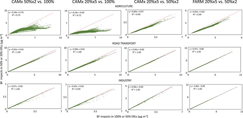
C. A. Belis et al.: Comparison of source apportionment approaches and analysis of non-linearity                               4737

Figure 3. Scatter plots of the single grid cell annual average BF source impacts (CAMx and FARM) on PM10 versus the TS contributions
(CAMx–PSAT) for 100 %, 50 % (multiplied by 2) and 20 % (multiplied by 5) ERLs for AGR, TRA and IND. Dotted line: regression; red
line: identity.

https://doi.org/10.5194/gmd-14-4731-2021                                               Geosci. Model Dev., 14, 4731–4750, 2021
4738                    C. A. Belis et al.: Comparison of source apportionment approaches and analysis of non-linearity

non-linear behaviour is associated with a situation near to         The non-linearity between TS and BF source apportion-
double counting, which results in negative interaction terms,    ment of PM10 secondary inorganic constituents observed in
and for nitrate, also near to the NH4 NO3 equilibrium, since     Figs. S5–S7 occurs when the BF and TS approaches do not
both effects lead to BF impacts higher than TS contributions     allocate these compounds to the same sources. For instance,
(Appendix A).                                                    high non-linearity is observed for BF impacts of TRA and
   Despite the comparable range of BF impacts and TS con-        IND on ammonium because it is emitted almost exclusively
tributions of AGR on PM10 at 50 % and 20 % ERLs (Fig. 3),        by AGR, while BF methods allocate impacts on ammonium
there is a considerable dispersion around the regression line    to TRA and IND due to the atmospheric reactions between
(R 2 between 0.65 and 0.72), indicating spatial heterogeneity.   NH3 and HNO3 or H2 SO4 , which are mainly emitted from
In addition, impacts at 20 % ERL present a slightly lower        TRA and IND, respectively. A similar situation is observed
slope with respect to TS contributions than those at 50 %        for AGR impacts on sulfate and nitrate. TS allocates a neg-
ERL. Also, AGR BF impacts on nitrate present non-linear          ligible share of these compounds to AGR (proportional to
high values at 50 % and 20 % ERLs, which are however com-        SO2 and NOx emissions from AGR only), while the BF
pensated for by ammonium impacts which are much lower            method allocates them to this source proportionally to the
than TS contributions (Figs. S6 and S7 in the Supplement, re-    (NH4 )2 SO4 and NH4 NO3 concentration variations, respec-
spectively). The greater difference observed between TS and      tively.
BF at 100 % ERL for AGR compared to TRA and IND is in               The analysis of the impacts reported in this section clearly
part due to AGR being the only significant source of NH3         points to AGR as the source mostly associated with the non-
in the domain. Consequently, a 100 % reduction in AGR im-        linear response of BF impacts with respect to TS.
plies an almost complete abatement of NH3 , while 100 % re-
duction in TRA or IND does not reduce NOx and SO2 emis-          3.2   Non-linearity between different ERLs
sions completely (compensation effect). The reported differ-
ences between AGR TS contributions and BF impacts on             In this section the connection between the magnitude of the
PM10 concentrations are due to the way in which the two          emission reduction and the BF source impacts on PM10 is
approaches allocate ammonium, nitrate and sulfate to this        analysed more in detail. The scatter plots in Fig. 4 depict
source. TS allocates secondary constituents according to the     the relationships between BF impacts at different ERLs for
mass of precursors deriving from each source (Mircea et al.,     every source and model. IND is the source for which the
2020; Yarwood et al., 2004). Therefore, for TS the contri-       similarity between the different ERLs is the highest with re-
bution of AGR is close to the mass fraction of ammonium          gression slopes and R 2 between impacts calculated for the
in PM10 , and very little nitrate and sulfate is allocated to    three ERLs of CAMx and the two of FARM near unity. Al-
this source, since SO2 and NOx emissions from AGR are            though the regressions between TRA impacts are also linear,
small compared to those from IND and TRA. By contrast,           the 50 % ERL impacts are ca. 8 % lower and 20 % ERL ca.
BF allocates these constituents on the basis of the amount of    12 % lower than those obtained with 100 % ERL using the
NH4 NO3 and/or (NH4 )2 SO4 , which is not formed when such       same model. The impacts at 50 % and 20 % ERLs are well
sources are reduced. Consequently, considerable nitrate and      correlated, and the latter are less than 5 % below the former
sulfate are allocated to AGR by BF, even though they are not     for both CAMx and FARM values. For AGR the relation-
physically emitted by this source, because there is no forma-    ship between the impacts calculated for both 50 % and 20 %
tion of NH4 NO3 and/or (NH4 )2 SO4 in the absence of NH3         ERLs are clearly non-linear when compared to 100 % ERL.
emissions from AGR.                                              In the latter impacts are 3 or 4 times higher than the for-
   Even in the cases where BF impacts and TS contributions       mer two, especially for mid to high impacts. By comparison,
to PM10 are linear and close to identity, PM10 constituents      the relationship between impacts at 50 % and 20 % ERLs
may not behave in the same way. Sometimes, the linearity ob-     is closer to linearity (R 2 = 0.99), with the latter leading to
served in PM10 is the result of a compensation between con-      18 %–20 % lower impacts than the former. The results shown
stituents for which BF impacts > TS contributions and others     in Fig. 4 confirm that AGR is the source presenting the most
for which BF impacts < TS contributions. A good example          serious non-linearity among those emitting SIA precursors
is TRA, whose annual BF impacts on PM10 are aligned with         (see Sect. 3.1). In addition, the analysis indicates that also for
TS contributions (Fig. 3). However, the ammonium impacts         TRA the impacts of the different ERLs are not fully equiva-
from this source are highly non-linear and larger than TS        lent.
contributions (Fig. S7), sulfate impacts are quite non-linear       The large differences in AGR impacts on PM10 between
and can be either larger or smaller compared to TS contri-       100 % and the other ERLs are likely explained by two rea-
butions (Fig. S5), while nitrate impacts are rather linear and   sons. Firstly, turning off AGR 100 % systematically shifts
slightly lower than TS contributions (Fig. S6). A similar sit-   the system into a different chemical regime, while this is not
uation is observed for nitrate and ammonium impacts from         the case for the other sources, and secondly, the influence of
IND, with the difference that in this case sulfate, a compo-     limiting precursors (leading to less than double counting and
nent for which this source is dominant, is rather linear.        consequently less BF overestimation with respect to TS) is

Geosci. Model Dev., 14, 4731–4750, 2021                                           https://doi.org/10.5194/gmd-14-4731-2021
C. A. Belis et al.: Comparison of source apportionment approaches and analysis of non-linearity                              4739

Figure 4. Scatter plots of the single grid cell BF source impacts (CAMx and FARM) on PM10 between 100 %, 50 % (multiplied by 2) and
20 % (multiplied by 5) ERLs for AGR, TRA and IND. Dotted line: regression; red line: identity.

https://doi.org/10.5194/gmd-14-4731-2021                                              Geosci. Model Dev., 14, 4731–4750, 2021
4740                     C. A. Belis et al.: Comparison of source apportionment approaches and analysis of non-linearity

not expressed at 100 % ERL (Appendix A Sect. A2.2). The            proposed. Such an arbitrary threshold was defined to high-
differences between 50 % and 20 % ERLs could be explained          light the interactions that according to the analysis of the im-
by the way in which limited chemical regimes interact with         pacts presented in the previous sections are associated with
the reduction in emissions. Since the non-linearity associ-        evident non-linear situations (e.g. AGR–TRA). In Figs. S11
ated with limited chemical regimes appears only when the           and S12 in the Supplement are reported the maps of the in-
emission reduction causes a drop in concentrations higher          teraction terms expressed as a percentage of the base case for
than the excess of the non-limiting precursor (Appendix A),        100 % and 50 % ERLs, respectively. According to the pro-
the chance of such non-linearity influencing source impacts        posed threshold, at 100 % ERL most of the Po Valley falls
is proportional to the emission reduction. However, the rel-       in the area where non-linearity is measurable for all the bi-
atively small differences observed between 50 % and 20 %           nary and ternary interactions. At 50 % ERL, the non-linearity
ERLs are likely due to the smoothing effect of the NH4 NO3         of the binary interactions AGR–IND are measurable in in-
equilibrium with respect to the non-linearity caused by a lim-     dustrial districts located to the SW and NW of the Po Val-
ited chemical regime because such equilibrium leads PM10           ley, including the industrial areas to the NW of Milan. The
concentrations to change even when the non-limiting precur-        non-linearity associated with the interaction AGR–TRA is
sor emission reduction is lower than the excess (Appendix A        not negligible in the entire Po Valley and also in the Alpine
Fig. A1).                                                          areas, probably due to the low PM10 levels of the latter. The
                                                                   binary interaction IND–TRA exceeds the threshold only in
3.3    Interaction terms                                           the central area of the Po Valley and in a hotspot to the NW
                                                                   of Milan. The ternary interaction is below the threshold for
In Fig. 5 the annual average interaction terms (ĉ) of the fac-    the entire domain. For 20 % ERL (not shown), all the inter-
tor decomposition, which are used in this study as indica-         actions are negligible according to CAMx, while FARM pro-
tors of the impact’s non-linearity, are mapped. The binary         vides a pattern comparable to 50 % ERL.
interaction terms are, in general, of higher magnitude than
the ternary interaction terms. The most negative interaction       3.4   Analysis of chemical regimes
terms (indicating BF > TS) are observed in 100 % ERL for
the contemporary reduction in AGR and TRA in the rural ar-         A more in-depth analysis of the relationships between the
eas located to the north of the Po Valley where NH3 is in ex-      chemical regime and the interaction terms was accomplished
cess, while the interaction terms are less negative in the main    in three selected sites with different source emission set
urban areas, where NH3 is a limiting factor. When AGR and          up (their position is shown in Fig. S1). A rural location at
IND are both reduced by 100 %, the most negative interac-          the border between the provinces of Cremona and Brescia
tion terms are observed in the industrial districts around the     (CR_P) was selected because of the high NH3 emissions,
main cities to the south of the Po Valley and to a lesser extent   while the local NOx and SO2 emissions are very limited. The
in the rural areas in the central Po Valley. By contrast, posi-    site of Milan (MI) was selected because it is representative of
tive interaction terms are observed for the IND–TRA binary         a typical urban situation with high NOx concentrations deriv-
reduction due to the competition between HNO3 and H2 SO4           ing from road transport emissions. The NH3 emissions in this
that leads to an increase in the PM formation when SO2 emis-       site are very limited and are associated with road transport,
sions (mainly industrial) are reduced in the presence of NOx       while SO2 emissions are also low and derive in part from
(deriving mainly from road transport). Such maximum pos-           the energy production. The third site is an industrial area in
itive interactions are observed in vast areas of the central       the province of Ravenna (RA_P) located in the south-eastern
Po Valley. A similar geographical pattern of the interaction       Po Valley. In this location, there are considerable SO2 emis-
terms is observed for 50 % and 20 % ERL (Figs. S8 and S9           sions from industry, which also release NOx , and moderate
in the Supplement, respectively), with the magnitude of the        NH3 emissions from the agricultural sector. In order to define
interaction decreasing with the emission reduction.                the chemical regime in each base case (CAMx and FARM)
   A similar analysis was carried with FARM at 50 % ERLs           and each of the simulations including binary or ternary in-
for residential heating (Fig. S10 in the Supplement), and          teractions, the gas ratio (GR) proposed by Ansari and Pandis
the resulting interaction terms were very low compared with        (1998) was used:
those of the other sources at the same ERL. The explanation
                                                                                           2−
is that despite the considerable contribution of this source to    GR = ([NH3 ]+[NH+                        −
                                                                                   4 ]−2[SO4 ])/([HNO3 ]+[NO3 ]), (2)
PM10 , its origin is mainly primary with a high non-reactive
carbonaceous fraction (Piazzalunga et al., 2011), and there-       where concentrations are nmol m−3 or in nmol mol of air
fore the impact on the secondary inorganic aerosol is limited.     (ppb).
   The values of the interaction terms depend on the pol-            The GR value defines three different chemical regimes:
lutant concentration. In order to define when ĉ is signifi-
cantly different from zero, and consequently when the non-          (a) GR > 1, in which NH4 NO3 formation is limited by the
linearity is not negligible, the absolute value |0.5| % BC is           availability of HNO3 ,

Geosci. Model Dev., 14, 4731–4750, 2021                                            https://doi.org/10.5194/gmd-14-4731-2021
C. A. Belis et al.: Comparison of source apportionment approaches and analysis of non-linearity 4741
Figure 5. Map of the binary and ternary interaction terms of the PM10 factor decomposition for AGR, IND and TRA in the CAMx BF 100 %
scenarios.
(b) 0 < GR < 1, in which NH4 NO3 formation is limited by to ĉ values ≥ 0, consistent with the competition effect (Ap-
the availability of NH3 , and pendix A Sect. A2.3). In CR_P and RA_P such simulations
lead to increase in GR (data points in Fig. 6a and c are placed
(c) GR < 0, in which NH4 NO3 formation is inhibited by
to the right of their base case), while in MI they lead to null
H2 SO4 .
or slightly negative changes in GR (data points are located to
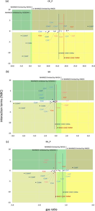
The plots in Fig. 6 display for each scenario the magnitude the left of the base case in Fig. 6b). This behaviour indicates
of the changes in the chemical regime with respect to the that the simultaneous reduction in IND and TRA leads to a
base case and the relationship between such changes and higher impact of ammonia + nitric acid on GR compared to
the interaction terms (expressed as a percentage of the PM the one of sulfate, in the three sites.
yearly mean concentrations). Each plot is divided into zones In CR_P the base cases of CAMx and FARM represent a
defined by the combination of the GR thresholds and the HNO3 -limited chemical regime for NH4 NO3 formation, in
threshold proposed in this study for the interaction terms (ĉ > line with the rural character of this area (Fig. 6a). All scenar-
|0.5 % BC|) as an indicator of non-negligible non-linearity in ios where AGR is reduced lead to a decrease in GR (points
the mass concentration allocated to sources with respect to located to the left of the corresponding base case), indicat-
the PM mass concentration. ing a loosening of the HNO3 limitation, while all those in
A common feature of all three sites is that the higher which AGR is not reduced lead to an increase in GR (points
the ERL, the higher the difference between the GR of the located to the right of the corresponding base case), indicat-
scenarios and the one of the base case providing evidence ing a stronger HNO3 limitation. Sizeable negative ĉ are ob-
about the extent to which the emission reductions alter the served in scenarios reducing AGR 100 %, likely associated
original conditions. The points representing simulations in with the shift towards a NH3 -limited regime when AGR, the
which AGR is reduced sit to the left of their respective base only significant source of this precursor, is turned off. The
case. The scenarios with 100 % ERL often lead to changes described situation is reflected by the points representing the
in the chemical regime and to the highest absolute interac- interaction terms AGR–IND (C10AI), AGR–TRA (C10AT)
tion terms. On the other hand, 50 % and 20 % ERLs lead, and AGR–IND–TRA (C10AIT) of 100 % ERL located in the
in general, to ĉ values closer to zero than 100 % ERL, in- bottom left of Fig. 6a. The only 100 % ERL scenario that
dicating lower or negligible non-linearity (located in the does not lead to a chemical regime change is the contem-
white background area). All interactions IND–TRA give rise
https://doi.org/10.5194/gmd-14-4731-2021 Geosci. Model Dev., 14, 4731–4750, 20214742 C. A. Belis et al.: Comparison of source apportionment approaches and analysis of non-linearity
porary reduction in IND and TRA (C10IT). It also leads to
positive interaction terms resulting from the competition be-
tween HNO3 and H2 SO4 . In this case, the abatement of SO2
emissions leads to a reduced availability of H2 SO4 , which is
replaced in the reaction with NH3 by HNO3 , the latter de-
riving from NOx emissions also from other sectors on top of
TRA and IND (e.g. energy industry), which is an example of
a compensation process (Appendix A Sect. A2.5). Figure 6a
shows that for 50 % and 20 % ERLs, the emission reductions
do not modify the chemical regime at this site. The AGR–
TRA (C5AT) is the only scenario at 50 % ERL leading to a
non-negligible ĉ value. The scenarios at 20 % ERL generally
show similar behaviours to those at 50 %.
In MI the base case simulations correspond to a chemi-
cal regime where NH4 NO3 is limited by NH3 (Fig. 6b). The
inhibition of NH4 NO3 formation by H2 SO4 is unclear since
the GR values calculated from both models are close to the
boundary between H2 SO4 inhibited and non-inhibited chem-
ical regimes. As in the previous site, all scenarios with 100 %
ERLs (C10) but one (C10IT) lead to a situation with strong
NH3 limitation, H2 SO4 inhibition and negative interaction
terms (data points in the bottom left of Fig. 6b). However, un-
like the previous site, the combined 100 % reduction in IND
and TRA (C10IT) in MI leads to a H2 SO4 -limited regime.
Thus, all 100 % ERL scenarios lead to a strengthening of the
H2 SO4 -inhibited chemical regime, which is relatively weak
in the base case. As already observed in CR_P, the interaction
terms at 50 % and 20 % ERLs are negligible, with the excep-
tion of AGR–TRA (C5AT). Among these scenarios, all those
involving AGR reductions lead to regimes where NH4 NO3
formation is limited by NH3 and inhibited by H2 SO4 (data
points to the left of the corresponding base case). By con-
trast, most scenarios not involving AGR (F5IT, F2IT, except
C5IT) lead to situations where NH4 NO3 formation is more
limited by NH3 (data points to the right of the corresponding
base case), while the inhibition by H2 SO4 is uncertain since
data points remain close to the boundary between the two
regimes.
In RA_P, both base cases are in a regime of NH4 NO3 for-
mation limited by NH3 . However, for CAMx base case sim-
ulation NH4 NO3 formation is not inhibited by H2 SO4 , while
this is the case for the FARM base case (Fig. 6c). As in CR_P,
the CAMx 100 % scenarios in which AGR is reduced lead to
a decrease in GR and negative interaction terms (data points
in the bottom left), while the one involving the interaction
IND–TRA (C10IT) leads to an increase in GR and positive
interaction terms (data points in the top right). All scenarios
Figure 6. Plot of the interaction terms (ĉ), expressed as a percentage
of the base case (BC), in three selected sites with different chemical
in which AGR is reduced lead to NH3 limitation and in most
regimes versus the gas ratio (Ansari and Pandis, 1998). (a) CR_P: cases also H2 SO4 -inhibition chemical regimes (data points
Cremona province, (b) MI: Milan and (c) RA_P: Ravenna province. to the left of the respective base case). By contrast, the sce-
C: CAMx and F: FARM. 10, 5 and 2 indicate 100 %, 50 % and narios in which only combustion sources (TRA and IND) are
20 % ERLs, respectively. A: agriculture, I: industry and T: trans- reduced lead to regimes where NH4 NO3 formation is limited
port. White background indicates negligible interaction terms. by NH3 (data points to the right of the corresponding base
case) and not inhibited by H2 SO4 (with some data points
close to the boundary between the two regimes).
Geosci. Model Dev., 14, 4731–4750, 2021 https://doi.org/10.5194/gmd-14-4731-2021C. A. Belis et al.: Comparison of source apportionment approaches and analysis of non-linearity 4743
Among the scenarios at 50 % and 20 % ERLs, those in- The factors that trigger differences in SA between the TS
volving AGR and IND lead to the highest absolute interac- and BF approaches also lead to non-linearity among differ-
tion terms, of which some (C5AI, F2AI) are negative and ent levels of emission reduction. For PM10 , this non-linearity
clearly different from zero (non-linearity), with the exception is higher between 100 % and the other reduction levels and
of F5AI, which presents a negligible interaction term. The is mainly observed in scenarios involving AGR reductions
higher interaction terms for the AGR–IND scenarios with re- where the differences may reach a factor of 3–4 and to a
spect to the other sites may be related to the greater impor- lesser extent in scenarios involving TRA where differences
tance of IND compared to TRA in this particular region. are ca. 10 %. This is due to (a) the almost complete suppres-
The numerical relationship between the interaction terms sion of NH3 when turning off AGR, while turning off TRA
and the gas ratio delta (i.e. the difference between the gas ra- leaves other strong sources of SO2 and NOx active, and (b)
tio in one run and the corresponding base case) varies from the fact that limiting precursors’ effects is only observable
site to site and, therefore, it is not possible to define accept- for ERLs below 100 %. Moreover, the present study shows
ability thresholds valid for the entire domain. that even when the secondary inorganic components of PM 10
present a non-linear behaviour in their annual averages, the
PM10 response may be linear due to the compensation be-
4 Conclusions tween different constituents.
It was also observed that in the majority of the tested sce-
The theoretical analysis carried out by Clappier et al. (2017)
narios at 50 % and 20 % ERLs, interaction terms are either
applying factor decomposition was further developed in this
negligible or remain low (a few percent of the base case con-
study by undertaking a real source apportionment exercise
centrations). In these conditions, the TS and BF approaches
using CTM models in an area with a complex meteorology
provide comparable results. Such findings were confirmed in
and chemistry, namely the Po Valley.
this study by the direct comparison between these two ap-
The interaction terms of the factor decomposition measure
proaches that provided highly comparable spatial patterns
the consistency between the impacts obtained with single-
and quantification of the role (contribution or impact) of
source reductions compared to those of multiple-source re-
IND, TRA and RES sources.
ductions. Consequently, they are also suitable indicators of
Due to its high emission levels and stagnation of air
the non-linearity between the sum of the sources’ mass con-
masses, the situations potentially leading to non-linear re-
centration and the PM10 total mass concentration. In addi-
sponses are common in the Po Valley, making this region par-
tion, the interaction terms used in association with the GR
ticularly suitable for studying these kinds of phenomena. The
provide evidence about the relationships between changes
results of the study suggest that AGR is the most important
in the chemical regime (e.g. limiting precursor, competition)
source from this point of view: a number of scenarios involv-
and the non-linear response of PM10 concentrations to emis-
ing the reduction in emission from AGR lead to non-linear
sion reductions.
responses of PM10 . This is due to the key role of NH3 , whose
The analysis of the single secondary inorganic constituents
only significant source is AGR in the formation of secondary
of PM10 combined with interaction terms and GR made it
inorganic aerosol (SIA) in the test area. In addition, scenar-
possible to identify a series of mechanisms that influence
ios with high AGR emission reduction (e.g. 100 %) lead to a
the non-linear response of these pollutants when emission
shift of the NH4 NO3 formation chemical regime. One of the
reduction scenarios are applied to a real particulate pollu-
implications of these findings is that when there is a strong
tion case: near double counting, a precursor-limited chemi-
non-linear response (e.g. 100 % reduction in AGR), it is not
cal regime, competition between precursors, thermodynamic
appropriate to sum the impacts obtained with single-source
equilibrium and compensation.
reductions to estimate the combined effect of more than one
The results of this study confirm that due to the key role of
source. Furthermore, in the case of AGR emission reduc-
NH3 in the formation of SIA in the Po Valley, the strongest
tion, extrapolating the results of moderate ERL scenarios to
non-linear response of PM 10 concentrations to emission re-
stronger ERL (e.g. greater than 50 %, as shown in Fig. 4) is
ductions is associated with the AGR–TRA reduction scenar-
discouraged too. Likewise, in such situations, the use of TS
ios. The differences in PM10 attributed to AGR applying the
results to derive information about emission reduction impact
TS and the BF approaches at the 100 % emission reduction
can be misleading.
level reach a factor 2. Moreover, the competition between
The findings of the present work about PM10 are also valid
HNO3 and H2 SO4 to react with NH3 leads to a modest non-
for the behaviour of PM2.5 . In the runs used for this study
linear response of PM10 in scenarios where TRA and IND are
these two size fractions present the same geographical pat-
reduced simultaneously, especially in areas with important
terns and values because the difference between them (the
SO2 emissions. Tests carried out in the study area about RES
coarse fraction) is mainly primary and thus expected to re-
indicate very little non-linearity associated with this source,
spond linearly to emission reduction.
likely due to the dominance of the primary fraction, includ-
Considering the complexity of computing the Stein and
ing a considerable amount of carbonaceous constituents.
Alpert decomposition for all possible combinations of source
https://doi.org/10.5194/gmd-14-4731-2021 Geosci. Model Dev., 14, 4731–4750, 20214744 C. A. Belis et al.: Comparison of source apportionment approaches and analysis of non-linearity
reductions (due to the high number of required runs), this Moreover, in the case of non-linear responses, also extend-
work aims to provide a picture of the conditions that give ing the results of BF for a specific ERL to another (e.g. 20 %
rise to non-linear responses of PM10 or PM2.5 yearly aver- to 50 % or 100 %) could be misleading.
ages for the reduction in single sources. Such a picture is in- To overcome the limitations of strong non-linear responses
tended as a contribution to simplify the tests needed in com- on source apportionment, the only option is to run a scenario
mon modelling practice to detect non-linear responses by al- analysis with the exact combination of emission reductions
lowing practitioners to focus on the situations that are more for all the sources at once so all the interactions among them
likely to be associated with non-linearity. leading to secondary compounds are accounted for. However,
BF and TS are different but complementary techniques. this approach is valid only for one specific situation.
Understanding how they work is necessary to adopt the one The methodology proposed in this study provides the
which is most suitable for the purposes of the work. On the means to identify non-linear responses to promote a more
one hand, BF is the best choice to assess the response of the mindful use of source apportionment techniques, the ultimate
air quality system to changes in the emission rates. For in- goal of which is to inform more effective air quality plans
stance, this approach emphasises better the key role of agri- with a consequent more efficient use of economic resources
culture and is then most suitable for planning purposes. On and a faster achievement of air quality standards to protect
the other hand, TS is most valuable when the focus is on the human health and ecosystems.
actual mass transferred from sources to receptors in the situ-
ation described in the base case. It is, therefore, most appro-
priate for studying the health impact of sources because the
effect of pollutants depends on the dose. An option to em-
phasise the role of agriculture with this approach would be
to develop a version based on the molar ratios instead of the
mass. However, assessing the usefulness of such an approach
would require a new full set of tests.
One of the main outcomes of this study is that in most
situations (linear response) the two approaches provide sim-
ilar results for the annual averages, which is the time aver-
aging required for long-term air quality indicators. However,
for shorter time windows (daily, seasonal averages or pollu-
tion episodes) non-linearity is likely to be more prominent.
If there is a clear non-linear response, precaution is needed
in the interpretation of the results from both approaches:
– in BF it is not appropriate to sum the impact of the
sources obtained by single-source reduction because
they may not match the total PM, while
– in TS there could be a distortion in the allocation of sec-
ondary aerosol because it does not account for indirect
effects (Mircea et al., 2020; Thunis et al., 2019).
Geosci. Model Dev., 14, 4731–4750, 2021 https://doi.org/10.5194/gmd-14-4731-2021C. A. Belis et al.: Comparison of source apportionment approaches and analysis of non-linearity 4745
Appendix A A2.1 Double counting
A1 Interaction terms This interaction takes place when the concentrations of the
emitted precursors (α, β) are close to the stoichiometric ra-
The interaction terms in the factor decomposition (Stein and tios and consequently none of them is limiting the reaction
Alpert, 1993) reflect the consistency between single-source or is in excess. In addition, no compensation mechanisms
emission reduction and contemporary reduction in more than (see Sect. A2.5) take place, and there are no other precursors
one source and are indicators of the non-linear response of competing for the reaction between α and β. Under these cir-
particulate matter (PM10 or PM2.5 ) concentration to single- cumstances, the application of the brute force (BF) approach
source reductions. leads to a 100 % reduction in the concentration of γ when re-
ducing the emissions of either source A or B by 100 %. This
A1.1 Binary interactions is called “double counting” because the sum of the scenario
where only A is reduced by 100 % and the one where only
Binary interactions describe the situation of two precursors α B is reduced by 100 % is exactly double the mass of the sce-
and β emitted by two different sources A and B, respectively, nario when both sources A and B are reduced at once. This
that react in the atmosphere to form the secondary compound situation is described in the equation below:
γ (α + β → γ ). 1C denotes the change in the concentration
of γ as a consequence of applying the same percentage of 1CAB = 1/2(1CA + 1CB ). (A6)
reduction to sources A and B separately or at the same time.
The binary interaction term (ĉAB ) is the difference between In other words, the 1C of the contemporary reduction in A
1C(γ ) due to the contemporary reduction in both sources and B is half of the sum of the 1C of the single reductions of
and the sum of 1C(γ ) due to the reduction in each single A and B, respectively. In this situation, ĉAB is negative, and
source: its absolute value is highest and is equal to the 1C of A and
B, which are equal to each other.
ĉAB = 1CAB − 1CA − 1CB . (A1)
ĉAB = −1CA = −1CB = −1/2(1CA + 1CB ) (A7)
A1.2 Ternary interactions
By analogy, ternary interactions refer to the interplay of three A perfect double counting is a theoretical situation that does
sources A, B and C, each emitting one precursor (α, β and not take place in the “real-world” formation of secondary in-
χ, respectively), which react among each other in the atmo- organic aerosol (SIA) because of the influence of other fac-
sphere for example as follows. tors such as reversible reactions and pH feedback on solubil-
ity (deliquescent particles). Consequently, in this study we
α + β → γ1 (A2) observe situations near to double counting where the inter-
action terms are strongly negative, like the one described be-
2α + χ → γ2 (A3)
low.
γ = γ1 + γ2 (A4) Let us consider the reaction NH3 + HNO3 → NH4 NO3 ,
where A is the source of NH3 and B is the one of HNO3 ,
The ternary interaction term is a function of 1C(γ ), result- and concentrations in ppb are denoted by [NH3 ] = a and
ing from the reduction in all three sources at once, of 1C(γ ) [NO3 ] = b. When setting the gas ratio (GR, Ansari and Pan-
resulting from the reduction in each single source at a time, dis, 1998) = 1, [SO2− −3
4 ] = 0.5 ppb (about 2 µg m ), and as-
and of the ĉ for all the combinations of binary source reduc- sume particles to be deliquescent, then d[PM]/d[NH3 ] =
tions as described below (see also Eq. 1): 2.5 and d[PM]/d[NO3 ] = 0.6. Under these circumstances,
a 50 % reduction in source A leads to a decrease in PM of
ĉABC = 1CABC − 1CA − 1CB − 1CC − ĉAB − ĉAC − ĉBC . 1CA = 2.5×a/2; a 50 % reduction in source B leads to a de-
(A5) crease in PM of 1CB = 0.6 × b/2, and a simultaneous 50 %
decrease in emissions from both A and B leads to a PM de-
A2 Situations giving rise to non-linearity crease in 1CAB = a/2 + b/2. The actual interaction term is
This section analyses in detail the situations that may lead ĉAB_actual = 1CAB − 1CA − 1CB = −0.75a + 0.2b,
to non-linearity. Most of these situations are visible in bi-
nary interactions; however, competition is only observable in while according to Eq. (A7) the double-counting interaction
ternary interactions. The different binary interactions that are term is ĉAB_DC = −0.625a − 0.15b.
part of ternary interactions may represent different situations Since near the stoichiometric ratio a is similar to b, the
described in this section, some of which lead to non-linearity actual interaction term is close to but less negative than the
and others not. double-counting interaction term.
https://doi.org/10.5194/gmd-14-4731-2021 Geosci. Model Dev., 14, 4731–4750, 20214746 C. A. Belis et al.: Comparison of source apportionment approaches and analysis of non-linearity
A2.2 Precursor-limited chemical regime In situations where the formation of SIA is not limited,
neither by H2 SO4 nor by HNO3 availability (and conditions
Most commonly, the concentrations of the precursors signif- are favourable to the formation of (NH4 )2 SO4 ), the reaction
icantly differ from the stoichiometric ratio, and consequently H2 SO4 + NH3 produces 1 mol of (NH4 )2 SO4 every 2 mol
one of them acts as a limiting factor or limiting precursor (in of NH3 , while the reaction HNO3 + NH3 produces 1 mol of
the example below the one emitted by source A, which im- NH4 NO3 for every mol of NH3 . The yield of aerosol in terms
plies 1CA > 1CB ). In this case, the emission reduction can of mol of the second reaction is twice the one of the first
lead to two different situations. reaction. The difference of mass in µg m−3 is as follows.
(a) The reduction in the emissions causes a decrease in the
non-limiting precursor (β) concentration lower than or – The reaction 2NH3 + H2 SO4 → (NH4 )2 SO4 leads to
equal to its excess with respect to the limiting precursor 3.9 µg m−3 PM from 1 µg m−3 NH3 .
(α), leading to an interaction equal to zero because 1CB
is zero and 1CAB = 1CA .
– The reaction NH3 + HNO3 → NH4 NO3 leads to
ĉAB = 1CAB − 1CA − 1CB = 0 (A8) 4.7 µg m−3 PM from 1 µg m−3 NH3 .
In this case the potential interaction does not take place.
Consequently, when the SO2 emissions are reduced in an
(b) The reduction in the emissions of source B is enough to NH3 -limited regime and HNO3 replaces H2 SO4 to react with
reduce the concentration of precursor β by more than its NH3 , there is an increase in the PM concentration.
excess with respect to α, leading to a negative ĉAB with In order to quantify the abovementioned competition, it is
a lower absolute value than the double counting. necessary to compute the interaction between at least three
sources at once (Eq. A5).
0 > ĉAB > −1/2(1CA + 1CB ) (A9)
The competition in a three-source system may lead to neg-
In this case there is a situation of less than double count- ative 1C (= increase in PM10 ) for the single IND reduction
ing. scenarios, which results in positive binary IND–TRA inter-
action terms (see Sect. 3.4). The effect is also observed in the
Less than double counting is an intermediate situation be- TRA impact on sulfate and the IND impact on nitrate.
tween no interaction and the maximum interaction, which
is the double counting, and the interaction terms are always
A2.4 Equilibrium with solid NH4 NO3
negative.
The limitation regime can only be observed when source
reductions are less than 100 % because, unless the same pre- The analysis of the previous cases is valid for unidirectional
cursor is emitted by other sources or transported from other or irreversible chemical reactions. However, in the atmo-
areas (see Sect. A2.5), the complete removal of the precursor sphere the reaction products, nitrate and ammonium, are in
leads to the complete removal of its products. thermodynamic equilibrium with the reagents ammonia and
In the real world, situations where NH4 NO3 formation is nitric acid.
limited by free NH3 availability (GR < 1) or total nitrate
availability (GR > 1) are common. However, due to feed- HNO3 + NH3 ↔ (NO− +
3 , NH4 ) (A10)
back processes, the impact of reducing the emissions of a
non-limiting precursor is small but not null, while the one
of reducing the emissions of a limiting precursor may be The actual concentrations of reagents and products depend
smoothed by the NH4 NO3 equilibrium (see Sect. A2.4). on the ratio between the kinetics of the reaction in either di-
rection. For the conditions in which particulate ammonium
A2.3 Competition nitrate is in a solid state (non-deliquescent particles), the
equilibrium constant K of this reaction is the product of the
The interaction between two sources A and B can be affected reagent gas-phase concentrations [HNO3 (g)] and [NH3 (g)]:
by a third one C when the precursors emitted by the two
sources B and C compete to react with the one emitted by
K = [HNO3 (g)][NH3 (g)]. (A11)
source A (see Eqs. A2 and A3). In the formation of SIA,
there is competition between HNO3 and H2 SO4 to react with
NH3 to produce ammonium nitrate and ammonium sulfate, Any emission reduction leading to decreases in HNO3 and/or
respectively. HNO3 derives from NOx emissions emitted i.a. NH3 gas-phase concentrations by a factor q shall lead to the
by road transport (there are other sources), H2 SO4 mainly shifting of the equilibrium towards the gas phase (volatilisa-
comes from SO2 emitted by industry, and NH3 is mainly tion) of a concentration of ammonium nitrate 1C so that the
emitted from agriculture. equilibrium (K = [HNO3 (g)] × [NH3 (g)]) is reached again.
Geosci. Model Dev., 14, 4731–4750, 2021 https://doi.org/10.5194/gmd-14-4731-2021You can also read