Evaluation of the CAMS global atmospheric trace gas reanalysis 2003-2016 using aircraft campaign observations - ACP
←
→
Page content transcription
If your browser does not render page correctly, please read the page content below
Atmos. Chem. Phys., 20, 4493–4521, 2020
https://doi.org/10.5194/acp-20-4493-2020
© Author(s) 2020. This work is distributed under
the Creative Commons Attribution 4.0 License.

Evaluation of the CAMS global atmospheric trace gas reanalysis
2003–2016 using aircraft campaign observations
Yuting Wang1,a, , Yong-Feng Ma2, , Henk Eskes3 , Antje Inness4 , Johannes Flemming4 , and Guy P. Brasseur1,5
1 Max  Planck Institute for Meteorology, 20146 Hamburg, Germany
2 Department  of Mechanics & Aerospace Engineering, Southern University of Science and Technology, Shenzhen, China
3 Royal Netherlands Meteorological Institute, De Bilt, the Netherlands
4 ECMWF, Shinfield Park, Reading, RG2 9AX, UK
5 National Center for Atmospheric Research, Boulder, CO, USA
a now at: Department of Civil and Environmental Engineering, the Hong Kong Polytechnic University,

Hung Hom, Kowloon, Hong Kong
 These authors contributed equally to this work.

Correspondence: Guy P. Brasseur (guy.brasseur@mpimet.mpg.de)

Received: 11 September 2019 – Discussion started: 8 October 2019
Revised: 3 March 2020 – Accepted: 20 March 2020 – Published: 17 April 2020

Abstract. The Copernicus Atmosphere Monitoring Service           1   Introduction
(CAMS) operated by the European Centre for Medium-
Range Weather Forecasts (ECMWF) has produced a global
                                                                 Global reanalyses of the chemical composition of the at-
reanalysis of aerosol and reactive gases (called CAMSRA)
                                                                 mosphere are intended to provide a detailed and realistic
for the period 2003–2016. Space observations of ozone, car-
                                                                 view of the three-dimensional distribution and evolution of
bon monoxide, NO2 and aerosol optical depth are assimi-
                                                                 the concentrations of the chemical species over a period
lated by a 4D-Var method in the 60-layer ECMWF global
                                                                 of several years. Information provided by advanced mod-
atmospheric model, which for the reanalysis is operated at a
                                                                 els in which different observational data are assimilated
horizontal resolution of about 80 km. As a contribution to
                                                                 is provided at rather high spatial and temporal resolutions
the evaluation of the reanalysis, we compare atmospheric
                                                                 (typically 80–110 km and 3–6 h, respectively). The Coper-
concentrations of different reactive species provided by the
                                                                 nicus Atmosphere Monitoring Service (http://atmosphere.
CAMS reanalysis with independent observational data gath-
                                                                 copernicus.eu, last access: 1 March 2020; CAMS), operated
ered by airborne instrumentation during the field campaigns
                                                                 by the European Centre for Medium-Range Weather Fore-
INTEX-A, INTEX-B, NEAQS-ITCT, ITOP, AMMA, ARC-
                                                                 casts (ECMWF) on behalf of the European Commission,
TAS, VOCALS, YAK-AEROSIB, HIPPO and KORUS-AQ.
                                                                 is currently producing a new global reanalysis of aerosols
We show that the reanalysis rather successfully reproduces
                                                                 and reactive trace gases (referred to as CAMSRA). The cur-
the observed concentrations of chemical species that are as-
                                                                 rently released reanalysis of aerosols and reactive gases cov-
similated in the system, including O3 and CO with biases
                                                                 ers the period 2003–2016 (Inness et al., 2019) and has re-
generally less than 20 %, but generally underestimates the
                                                                 cently been extended to 2017 and 2018 (Christophe et al.,
concentrations of the primary hydrocarbons and secondary
                                                                 2019); this reanalysis run will be continued close to real
organic species. In some cases, large discrepancies also exist
                                                                 time. The ECMWF has produced several other atmospheric
for fast-reacting radicals such as OH and HO2 .
                                                                 composition (AC) reanalyses. The earlier Monitoring Atmo-
                                                                 spheric Composition and Climate (MACC) project produced
                                                                 the MACC reanalysis (MACCRA) for the period of 2003–
                                                                 2012 (Inness et al., 2013; Stein et al., 2012). The CAMS in-
                                                                 terim reanalysis (CIRA) is a test product implemented af-

Published by Copernicus Publications on behalf of the European Geosciences Union.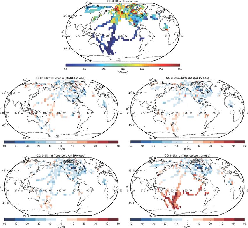
4494                         Y. Wang et al.: Evaluation of the CAMS global atmospheric trace gas reanalysis 2003–2016

ter the retirement of the coupled Integrated Forecast Sys-       The photolysis of ozone followed by the reaction of the re-
tem (IFS-MOZART; Flemming et al., 2009) and its replace-         sulting electronically excited oxygen atom with water vapor
ment by the IFS with online integrated chemistry and aerosol     (H2 O) represents the main sink of tropospheric O3 (Sheel
schemes (Flemming et al., 2015). The CIRA is available           et al., 2016). Carbon monoxide, either emitted at the sur-
from 2003 to 2018 (Flemming et al., 2017). The CAMSRA            face by incomplete combustion of fossil fuels and biomass
is built on the experience gained during the production of       burning or produced in the atmosphere as a result of the ox-
these two previous versions of the reanalysis, MACCRA and        idation of hydrocarbons (Khalil and Rasmussen 1984, 1990;
CIRA.                                                            Fortems-Cheiney et al., 2011), is destroyed mainly by reac-
   The validation of the CAMSRA is routinely performed by        tion with the OH radical (Pressman and Warneck, 1970). In
the CAMS validation team through the CAMS-84 contract            this paper, we mainly evaluate the concentration of O3 and
coordinated by KNMI (Christophe et al., 2019; Eskes et al.,      CO produced by all the three reanalyses by comparing them
2015, 2018). The validation uses various measurements, in-       with atmospheric observations made along flight tracks dur-
cluding satellite observations, ground-based remote sensing      ing past field campaigns (see Table 2). These comparisons
and in situ measurements, ozone soundings, and commer-           are performed in different regions of the world.
cial aircraft measurements, to assess the performance of the        Other chemical species (NOx , HOx , organics) produced
model versions and the reanalysis. The validation results for    by the CAMSRA are also evaluated at selected locations. The
CAMSRA 2003–2016 using these operational measurements            hydrocarbons considered are ethene (C2 H4 ), ethane (C2 H6 )
are shown by Eskes et al. (2018). The purpose of our paper       and propane (C3 H8 ). Secondary organic compounds, in-
is to report on the validation of the CAMSRA by using air-       cluding methanol (CH3 OH), acetone (CH3 COCH3 ), ethanol
craft measurements performed during past field campaigns         (C2 H5 OH) and methyl hydroperoxide (CH3 OOH), are the
in different parts of the world.                                 products of hydrocarbons and CO oxidation. Peroxyacetyl
   In contrast to long-term operational monitoring, aircraft     nitrate (PAN) and nitric acid (HNO3 ) are produced by pho-
campaigns are designed to address specific scientific ques-      tochemical reactions involving NOx (Emmons et al., 2000).
tions and perform intensive measurements in a specific re-       Hydrogen peroxide (H2 O2 ) represents a major tropospheric
gion during a limited period of time. Aircraft campaigns are     sink for HOx radicals. Formaldehyde (HCHO) is mainly pro-
therefore valuable supplements to evaluate the models and        duced by the oxidation of hydrocarbons but is also directly
in particular the reanalyses. Another advantage of intensive     emitted to the atmosphere from industry sources; it has a
campaigns is that they provide the opportunity to measure        substantial impact on the HOx concentration. By comparing
the concentrations of the chemical species that are not op-      these species, the underlying processes in the model can be
erationally monitored. The observations of these additional      further evaluated.
species can be used to better investigate the performance of
the models, in particular their ability to represent some com-
plex physical and chemical processes (Emmons et al., 2000).      2   Model description
   Ozone (O3 ) and carbon monoxide (CO) are two of the
main chemical species that are simulated in the three reanal-    Three versions of the global reanalysis are evaluated by con-
yses (MACCRA, CIRA and CAMSRA). Satellite measure-               ducting a comparison of the calculated fields with available
ments of these species are assimilated in these three reanal-    measurements made from aircraft during selected field cam-
yses, resulting in analyzed concentrations forced by obser-      paigns. Some of the key setups of these three reanalyses are
vations (Inness et al., 2019) but with constraints that dif-     listed in Table 1. The chemical schemes adopted for the re-
fer from species to species: these are strong in the case of     analysis models are the MOZART-3 mechanism (Kinnison
CO and stratospheric ozone but weaker in the case of tro-        et al., 2007) in the case of MACCRA and a modified ver-
pospheric ozone and NO2 (due to the short lifetime of this       sion of the Carbon Bond 2005 chemistry mechanism (Huij-
last species; Inness et al., 2015). The weaker constraint in     nen et al., 2010) in the case of CIRA and CAMSRA. Surface
tropospheric ozone also results from the fact that the ob-       boundary conditions for the reactive gases are generally ex-
served ozone amount in this lower region of the atmosphere       pressed as emissions and deposition, and the account for bio-
is provided by the difference between the total and strato-      genic, anthropogenic and pyrogenic effects. Methane, carbon
spheric ozone columns. Knowledge of the distribution of          monoxide and OH are calculated interactively with, in the
ozone and CO is key for understanding the role of the chem-      case of methane, specified surface concentrations. More de-
ical and transport processes in the atmosphere. Ozone is         tails can be found in Inness et al. (2019). MACCRA covers
a key indicator of photochemical pollution. This molecule        the period 2003 to 2012, while CIRA and CAMSRA provide
is produced in the atmosphere by reactions between nitro-        three-dimensional global fields from 2003 to 2016. Thus, in
gen oxides (NOx =NO + NO2 ), CO and volatile organic com-        our analysis, the campaigns that took place after 2012 are ex-
pounds (VOCs) in the presence of sunlight. Hydrogen rad-         cluded when compared to MACCRA. The model resolution
icals (HOx =OH + HO2 ) play an important role in this non-       for MACCRA and CAMSRA is 80 km, while it is 110 km in
linear process (Jacob, 2000; Lelieveld and Dentener, 2000).      the case of CIRA. All three reanalyses are made with a 60-

Atmos. Chem. Phys., 20, 4493–4521, 2020                                           www.atmos-chem-phys.net/20/4493/2020/
Y. Wang et al.: Evaluation of the CAMS global atmospheric trace gas reanalysis 2003–2016                                 4495

vertical-level model and extend from the surface to the alti-     were set up on a WP-3D aircraft, and the details can be found
tude pressure of 0.1 hPa. Each reanalysis provides two dif-       in Fehsenfeld et al. (2006).
ferent outputs: an analysis and a 0–24 h forecast. These two         ITOP (Intercontinental Transport of Pollution) was the
fields were compared in the case of CAMSRA, and they ap-          European (UK, Germany, and France) contribution to the
pear to be very similar (not shown here). The time resolution     ICARTT project. In the present study, we collect the mea-
for the analysis fields is 6 h for MACCRA and CIRA and            surements made onboard the UK FAAM BAE-146 air-
3 h for CAMSRA. For the forecast fields, the time resolution      craft. The instrument information is provided by Cook et
is 3 h for all the reanalysis versions. To use same time res-     al. (2007).
olution for the three reanalyses, the forecast fields are used       INTEX-B (Intercontinental Chemical Transport Experi-
in this present study. The satellite datasets that are assimi-    ment – Phase B) was the second phase of the INTEX-NA
lated in CAMSRA are summarized in Table 2. O3 , CO and            experiment led by NASA. In March of 2006, INTEX-B op-
NO2 are assimilated in CAMSRA, and each species is as-            erated in support of the multi-agency MIRAGE/MILAGRO
similated independently from the others (Inness et al., 2019).    (The Megacity Initiative: Local and Global Research Obser-
O3 total-column, stratospheric partial-column and profile re-     vations; Molina et al., 2010) project with a focus on ob-
trievals from several satellites are used to constrain mainly     servations in and around Mexico City. In its second phase,
the stratospheric O3 . As indicated above, the tropospheric       INTEX-B focused on the east coast of the US and on the Pa-
forcing is weaker because the information is provided by the      cific Ocean during the spring of 2006 (Singh et al., 2009).
residual between the total and stratospheric columns (Inness      The NCAR component of MILAGRO was MIRAGE-Mex
et al., 2015). The MOPITT total-column CO retrievals are          (Megacities Impact on Regional and Global Environment),
assimilated in CAMSRA, and the retrievals are mostly sensi-       and NCAR also contributed to INTEX-B. The NASA mea-
tive in the middle and upper troposphere (Deeter et al., 2013),   surement platform was the DC-8 research aircraft. The mea-
leading to the strongest constraint in that region. MOPITT        surement approaches for the selected species were the same
data used in the CAMS assimilation cover only the latitudes       as those adopted for INTEX-A. The NCAR measurements
between 65◦ N and 65◦ S, so the constraints are weak at high      were made from the NSF/NCAR C-130 airplane. The mea-
latitudes. For NO2 , the impact of the assimilation is small      surement method is described by Singh et al. (2009).
because the lifetime of NO2 is short (Inness et al., 2015). An       AMMA (African Monsoon Multidisciplinary Analysis)
additional control run for CAMSRA without data assimila-          was an international project to improve our knowledge and
tion is also evaluated to separate the impact of the assimila-    understanding of the West African monsoon (Lebel et al.,
tion from the other model-related factors.                        2010). Measurements to investigate the chemical composi-
   When comparing the concentrations calculated in the re-        tion of the middle and upper troposphere in West Africa dur-
analyses with the campaign data, the 4D model grid points         ing the July to August 2006 campaign were performed by the
(space and time) that are considered are those that are closest   UK FAAM BAE-146 aircraft, and the details are described
to the measurement locations (latitude, longitude and pres-       by Saunois et al. (2009).
sure layer) and times.                                               ARCTAS (Arctic Research of the Composition of the Tro-
                                                                  posphere from Aircraft and Satellites) was conducted during
                                                                  April and July 2008 by NASA (Jacob et al., 2010). ARCTAS
3   Aircraft measurements                                         was part of the international POLARCAT program during
                                                                  the 2007–2008 International Polar Year (IPY). In the present
Several aircraft campaigns are used to validate the three         study, we use the measurements made onboard NASA DC-
CAMSRA presented above. These campaigns are briefly de-           8 research aircraft. The species measured during ARCTAS
scribed below and in Table 2.                                     were the same as during INTEX-A.
   INTEX-A (Intercontinental Chemical Transport Exper-               VOCALS (VAMOS Ocean–Cloud–Atmosphere–Land
iment – North America Phase A) was an integrated at-              Study) was an international program that is part of the
mospheric field experiment performed over the east coast          CLIVAR VAMOS (Variability of the American Monsoon
of the United States organized by NASA during July and            Systems) project. The VOCALS experiment was conducted
August 2004 (Singh et al., 2006). It has contributed to a         from 15 October to 15 November 2008 in the southeast
large ICARTT program (International Consortium for Atmo-          Pacific region (Allen et al., 2011). The NSF C-130 aircraft
spheric Research on Transport and Transformation; Fehsen-         was used during the campaign.
feld et al., 2006). During this campaign, chemical species           YAK-AEROSIB (Airborne Extensive Regional Observa-
were measured by different instruments onboard a DC-8 air-        tions in Siberia) was a bilateral cooperation activity coor-
plane. The measurement methodology for the trace gases can        dinated by researchers from LSCE in France and IAO in
be found in Singh et al. (2006).                                  Russia. It aims to establish systematic airborne observations
   NEAQS-ITCT (New England Air Quality Study – Inter-             of the atmospheric composition over Siberia. In the present
continental Transport and Chemical Transformation) was the        study, we used the O3 and CO measurements during 2006–
NOAA component to the ICARTT program. The instruments             2008 and in 2014. The program used a Tupolev Tu-134 air-

www.atmos-chem-phys.net/20/4493/2020/                                             Atmos. Chem. Phys., 20, 4493–4521, 2020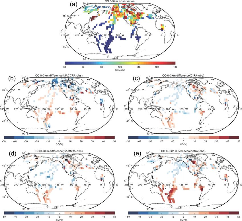
4496                                      Y. Wang et al.: Evaluation of the CAMS global atmospheric trace gas reanalysis 2003–2016

Table 1. Key setups of the three reanalyses.

     Reanalysis                             MACCRA                                         CIRA                                           CAMSRA
     Period                                 2003–2012                                      2003–2018                                      2003–present
     Spatial resolution                     80 km                                          110 km                                         80 km
     Vertical resolution                    60 levels                                      60 levels                                      60 levels
     Temporal resolution                    6-hourly analysis fields                       6-hourly analysis fields                       3-hourly analysis fields
                                            3-hourly forecast fields from                  3-hourly forecast fields from                  3-hourly forecast fields from
                                            00:00 UTC up to 24 h                           06:00 and 18:00 UTC up to 12 h                 00:00 UTC up to 48 h
     Assimilation system                    IFS Cycle 36r1 4D-Var                          IFS Cycle 40r2 4D-Var (2003–                   IFS Cycle 42r1 4D-Var
                                                                                           2015) and IFS Cycle 41r1 4D-
                                                                                           Var (2016–2018)
     Chemistry module                       MOZART3 (Kinnison et al.,                      CB05 and Cariolle ozone pa-                    CB05 with updates and Cari-
                                            2007)                                          rameterization in the strato-                  olle ozone parameterization in
                                                                                           sphere (Huijnen et al., 2010)                  the stratosphere (Huijnen et al.,
                                                                                                                                          2010)
     Anthropogenic emissions                MACCity (Granier et al., 2011)                 MACCity and CO emission up-                    MACCity and CO emission up-
                                                                                           grade (Stein et al., 2014)                     grade (Stein et al., 2014)
     Biogenic emissions                     Monthly mean VOC emissions                     Monthly mean VOC emissions                     Monthly mean VOC emissions
                                            by MEGAN2.1 (Guenther et                       by MEGAN2.1 using MERRA                        by MEGAN2.1 using MERRA
                                            al., 2006) for the year 2003                   reanalysis meteorology for                     reanalysis meteorology for the
                                                                                           2003–2010; a climatology                       whole period
                                                                                           dataset of the MEGAN-MACC
                                                                                           for 2011–2017
     Biomass burning                        GFED (2003–2008) & GFAS                        GFAS v1.2                                      GFAS v1.2
     emissions                              v0 (2009–2012)

Table 2. The satellite datasets of trace gases assimilated in CAMSRA.

  Species          O3                        O3                       O3                             CO                          CO                            NO2
                   (stratosphere)            (UTLS)                   (free troposphere)             (free troposphere)          (surface and PBL)             (free troposphere)
  Satellites       MIPAS, MLS,               Indirectly con-          Indirectly      con-           MOPITT                      Indirectly      con-          SCIAMACHY,
                   SCIAMACHY,                strained     by          strained by limb and                                       strained by satellite         OMI, GOME-2
                   GOME-2A,                  limb and nadir           nadir sounders                                             IR sounders
                   GOME-2B,                  sounders
                   OMI, SBUV-2
 Note: indirectly constrained means that there are no data in this layer assimilated for this species, but there is some impact coming from the residual of combining the datasets from
 the other layers.

craft. The detailed measurement techniques can be found in                                      NASA DC-8. The species were measured as during
Paris et al. (2008, 2010).                                                                      the INTEX-A campaign. A further description of this
   HIPPO (HIAPER Pole-to-Pole Observations), supported                                          field campaign can be found in the KORUS-AQ White
by the NSF and operated NCAR, used the NSF/NCAR G-V                                             Paper (https://espo.nasa.gov/korus-aq/content/KORUS-AQ_
aircraft. During five missions from 2009 to 2011 in different                                   Science_Overview_0, last access: 10 July 2019).
seasons, a large number of chemical species were observed                                          Since the goal of the present study is to evaluate the differ-
between the Arctic and the Antarctic over the Pacific Ocean.                                    ent ECMWF reanalyses by comparing the calculated fields
The details can be found in Wofsy et al. (2012).                                                with observations conducted during different campaigns and
   KORUS-AQ (Korea–US Air Quality Study) was a                                                  using different instruments, it is important to state that the
joint Korea and US campaign that took place in South                                            measurements of the major species are comparable. The dif-
Korea from April to June 2016. The US contribution                                              ferent instruments deployed during these campaigns were all
was led by NASA, and the aircraft platform was the                                              carefully calibrated, and in the case of ozone and carbon

Atmos. Chem. Phys., 20, 4493–4521, 2020                                                                                  www.atmos-chem-phys.net/20/4493/2020/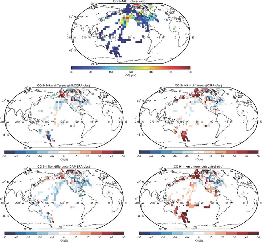
Y. Wang et al.: Evaluation of the CAMS global atmospheric trace gas reanalysis 2003–2016                                       4497

                                                                    pogenic emissions of ozone precursors (air pollution). In the
                                                                    9–14 km layer, the polar ozone concentrations are very high
                                                                    because the height of the tropopause in that region is lower
                                                                    than at lower latitudes, and as a result, the aircraft penetrated
                                                                    the ozone-rich stratosphere. The comparison between the air-
                                                                    craft observations and the reanalysis values from MACCRA
                                                                    is generally good. In the low troposphere, the biases of the
                                                                    averaged grids are mostly within 20 %. MACCRA underes-
                                                                    timates the O3 concentrations in the Arctic region and in the
                                                                    Southern Hemisphere, while it overestimates the O3 concen-
                                                                    trations in the northern low and middle latitudes, especially
                                                                    over the western Pacific Ocean (over 50 %), the eastern coast
                                                                    of US and the North Atlantic (about 40 %). The biases of
Figure 1. Flight tracks of the campaigns with the altitude of the   MACCRA in the middle troposphere are smaller than those
corresponding flight.                                               in the low troposphere. The positive biases in the lower layer
                                                                    become smaller with increasing altitude everywhere except
                                                                    in the Arctic, where the negative biases turn to positive val-
monoxide, for example, the quoted uncertainties in the mea-         ues. In the upper troposphere, the agreement is worse than
surements are 3–5 and 2–5 ppb, respectively, depending on           in the lower layers. The biases are mostly positive over the
the instrument. When, for a given campaign, more than one           Pacific Ocean and negative in North America.
instrument was used, the quantitative values were compara-             The agreement of CIRA with the aircraft measurements is
ble and were averaged before being used in our analysis. This       similar to the agreement of MACCRA when using the same
was the case, for example, for the HIPPO campaign during            measurements before 2013. In the lowest layer, however, the
which ozone was measured by two different instruments and           mean bias of CIRA is slight smaller than that of MACCRA.
carbon monoxide by three instruments.                               The CIRA reanalysis overestimates the observation in the
   Information on the aircraft campaigns is summarized in           middle of the Pacific Ocean and northwest of the Atlantic
Table 3. The flight tracks are shown in Fig. 1.                     Ocean, which is similar to the values derived from MACCRA
                                                                    but with smaller biases; CIRA underestimates ozone concen-
                                                                    trations in the rest of the region with biases of less than 20 %.
4     Evaluation of spatial distributions of chemical species
                                                                    Above the Pacific Ocean, the positive bias, which is small in
In the present section, we first evaluate the CAMSRA by             the lower layers of the atmosphere, increases with height and
comparing the calculated (reanalyzed) and observed con-             becomes substantial in the upper troposphere. The patterns
centrations of ozone, carbon monoxide and other chemical            of the biases in the CIRA reanalysis in the upper troposphere
species in different regions of the world during the selected       are similar to those in the middle troposphere layer but with
field campaigns. Carbon monoxide and ozone were mea-                larger values.
sured in all the field campaigns considered in the present             In the low troposphere, CAMSRA generally overestimates
study. Data are available in both hemispheres but princi-           the O3 concentration relative to the observation, which is
pally in the regions of North America, eastern Asia, Australia      different from the MACCRA and CIRA cases. The biases
and across the Pacific Ocean. In the case of nitrogen oxides,       of CAMSRA are usually less than 15 %, and the relatively
hydroxyl and peroxyl radicals, and formaldehyde, only the           larger biases are found in the tropics and Arctic, where the
measurements provided in North America, the northern Pa-            reanalysis overestimates the measurements by about 30 %.
cific and eastern Asia are considered here.                         In the free troposphere, the biases of the reanalysis become
                                                                    larger than in the low troposphere, especially over the trop-
4.1    Ozone                                                        ical ocean, while the differences are smaller in the western
                                                                    African region. For the comparison above 9 km, the positive
For the spatial evaluation, all the aircraft measurements and       biases over the Pacific Ocean are even larger and reach 50 %.
the extracted model data points are combined regardless of             The mean bias of the CAMS control simulation (model run
the time of the measurement; observations and models are            performed without assimilation of observed data) is similar
separated into three altitude layers: the low troposphere layer     to the bias associated with CAMSRA, but the patterns are dif-
(0–3 km), the middle troposphere layer (3–9 km) and the up-         ferent. The bias of CAMSRA is more uniform over the globe,
per troposphere–lower stratospheric layer (9–14 km).                which shows that data assimilation improves the global dis-
   The comparison of O3 between the observation and the             tribution of the O3 concentration. In the low troposphere, the
reanalyses is shown in Figs. 2, 3 and 4. The tropospheric           bias of the control run is of the order of 15 %. The control
ozone concentration is higher in the Northern Hemisphere            run underestimates the measurements on the west coast of
than the Southern Hemisphere because of higher anthro-              US and in the south of the Pacific Ocean, where the ozone

www.atmos-chem-phys.net/20/4493/2020/                                                Atmos. Chem. Phys., 20, 4493–4521, 2020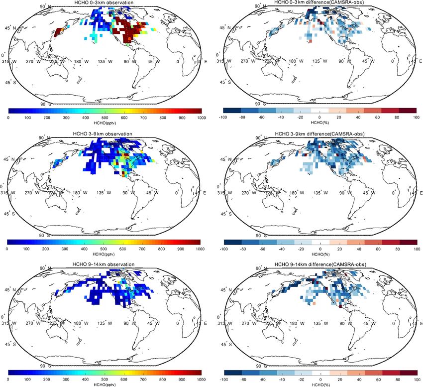
4498                                  Y. Wang et al.: Evaluation of the CAMS global atmospheric trace gas reanalysis 2003–2016

Table 3. List of aircraft campaigns used.

  Campaign                    Date              Location                  Species used                      Web page
  INTEX-A                     2004 Jul–Aug      Eastern America           O3 , CO, NO, NO2 , OH, HO2 ,      https://www-air.larc.nasa.gov/
                                                                          HCHO, H2 O2 , HNO3 , PAN,         missions/intexna/intexna.htm ∗
                                                                          C2 H4 , C2 H6 , C3 H8 , CH3 OH,
                                                                          CH3 COCH3 ,          CH3 OOH,
                                                                          C2 H5 OH
  NEAQS-ITCT                  2004 Jul–Aug      Eastern America           O3 , CO                           https://www.esrl.noaa.gov/csd/
                                                                                                            projects/2004/ ∗
  ITOP-UK                     2004 Jul–Aug      North Atlantic            O3 , CO                           http://artefacts.ceda.ac.uk/
                                                                                                            badc_datadocs/itop/itop.html ∗
  INTEX-B                     2006 Mar–May      Western America           O3 , CO, NO, NO2 , OH, HO2 ,      https://www-air.larc.nasa.gov/
                                                                          HCHO, H2 O2 , HNO3 , PAN,         missions/intex-b/intexb.html ∗
                                                                          C2 H4 , C2 H6 , C3 H8 , CH3 OH,
                                                                          CH3 COCH3 ,          CH3 OOH,
                                                                          C2 H5 OH
  AMMA-UK                     2006 Jul–Aug      West Africa               O3 , CO                           http://artefacts.ceda.ac.uk/
                                                                                                            badc_datadocs/amma/amma.
                                                                                                            html ∗
  ARCTAS                      2008 Apr–Jul      North America to Arctic   O3 , CO, NO, NO2 , OH, HO2 ,      https://www-air.larc.nasa.gov/
                                                                          HCHO, H2 O2 , HNO3 , PAN,         missions/arctas/arctas.html ∗
                                                                          C2 H4 , C2 H6 , C3 H8 , CH3 OH,
                                                                          CH3 COCH3 , CH3 OOH
  VOCALS                      2008 Oct–Nov      Southeast Pacific         O3 , CO                           http://data.eol.ucar.edu/project/
                                                                                                            VOCALS ∗
  YAK-AEROSIB                 2006–2008, 2014   Russia                    O3 , CO                           https://yak-aerosib.lsce.ipsl.fr/
                                                                                                            doku.php ∗
  HIPPO                       2009–2011         Pacific                   O3 , CO                           https://hippo.ornl.gov/data_
                                                                                                            access ∗
  KORUS-AQ                    2016 Apr–Jun      Korea                     O3 , CO                           https://www-air.larc.nasa.gov/
                                                                                                            missions/korus-aq/index.html ∗
∗ last access: 10 July 2019

concentrations provided by the CAMSRA are higher than                      ing linear regression parameters. Fewer data are available
the observation. In the polar free troposphere, the control                when considering MACCRA because MACCRA includes in-
simulation provides concentration values that are lower than               formation only until the year 2012. To more directly compare
suggested by the observations with a bias of about 20 %; in                with MACCRA, the regression parameters for the other mod-
contrast to this, in the tropical region, the control simulation           els runs before 2013 are also given in the table. The correla-
overestimates ozone, which is similar to the corresponding                 tions of all three reanalysis cases are high, with squared cor-
estimates by CAMSRA. In the upper layer, the bias pattern                  relation coefficients larger than 0.9. The highest correlation is
is similar to that in the free troposphere, but the bias values            achieved with CAMSRA. The squared correlation coefficient
are larger.                                                                R 2 derived for the control simulation (0.89) is not substan-
   Overall, for ozone, the level of agreement between the ob-              tially smaller than in the three cases with assimilation (0.93).
servations and the three reanalyses and between the observa-               This suggests that the CAMS model in its control mode has
tions and the control run are similar, but the biases associated           good predictive capability but that, as expected, data assim-
with CAMSRA are more uniform in space. A linear regres-                    ilation slightly improves the calculated ozone fields. To ex-
sion was performed between all observed ozone data points                  clude the contribution of stratospheric ozone values in the
and ozone concentrations extracted from the three reanalyses               statistical analysis, the stratospheric data were filtered out
and from the control simulation. Table 4 lists the correspond-             and the statistical parameters recalculated. The squared cor-

Atmos. Chem. Phys., 20, 4493–4521, 2020                                                      www.atmos-chem-phys.net/20/4493/2020/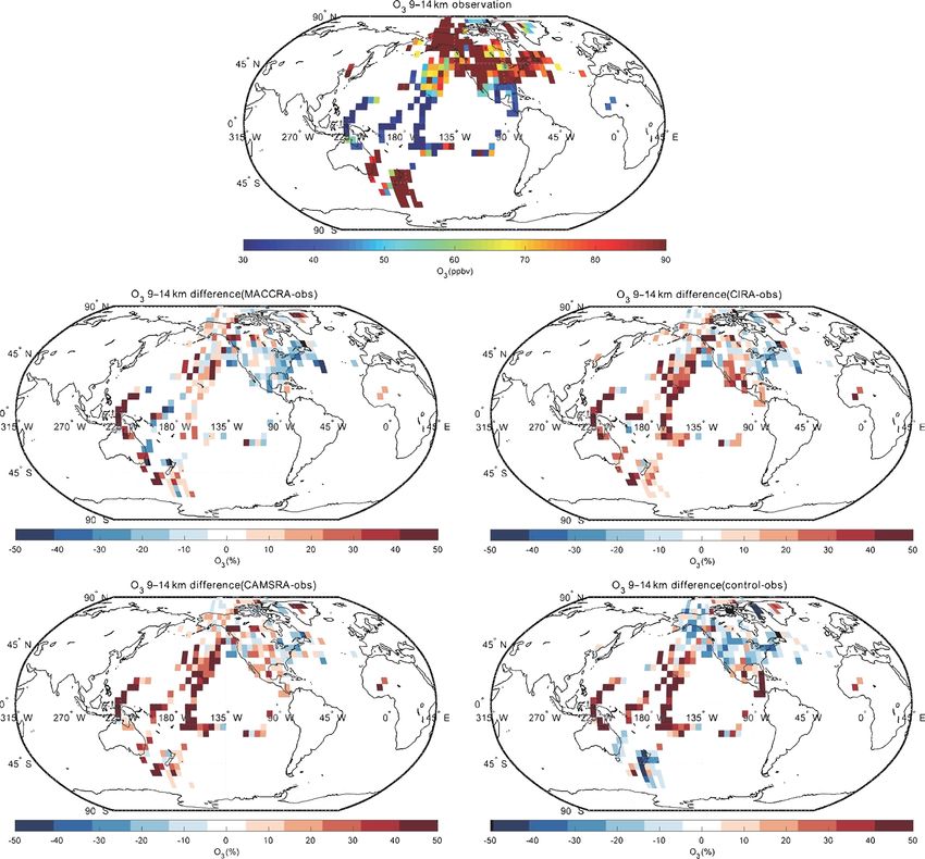
Y. Wang et al.: Evaluation of the CAMS global atmospheric trace gas reanalysis 2003–2016 4499
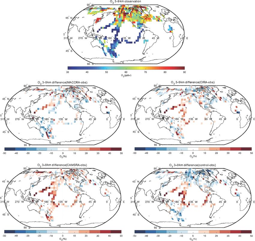
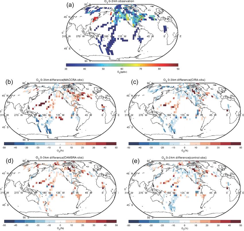
Figure 2. Campaign observations of O3 (a). (b) The relative difference in percent between MACCRA and the observations (MACCRA –
observation). (c) The difference between CIRA and the observations (CIRA – observation). (d) The difference between CAMSRA and the
observations (CAMSRA – observation), and (e) the difference between the control run and the observations (control – observation). The data
are averaged to 5◦ × 5◦ (latitude × longitude) and to the altitude bin of 0–3 km. Note that MACCRA only includes campaigns between 2003
and 2012.
relation coefficients decreased from about 0.9–0.95 to about gion and Canada (about 30 %), West Africa (about 20 %), and
0.6–0.7. the Southern Ocean (about 10 %). It overestimates the con-
centrations in the other regions covered by the campaigns,
4.2 Carbon monoxide with most of the biases within 15 %. In the middle tropo-
sphere, the bias pattern is similar to that of the low tropo-
The comparison of carbon monoxide between the observa- sphere, but the biases are smaller than in the lowest layer,
tion and the reanalyses is shown in Figs. 5, 6 and 7. MAC- especially in the Arctic. In the upper layer, often located in
CRA underestimates the CO concentrations in the Arctic re- the stratosphere, the biases become larger at high latitudes
www.atmos-chem-phys.net/20/4493/2020/ Atmos. Chem. Phys., 20, 4493–4521, 2020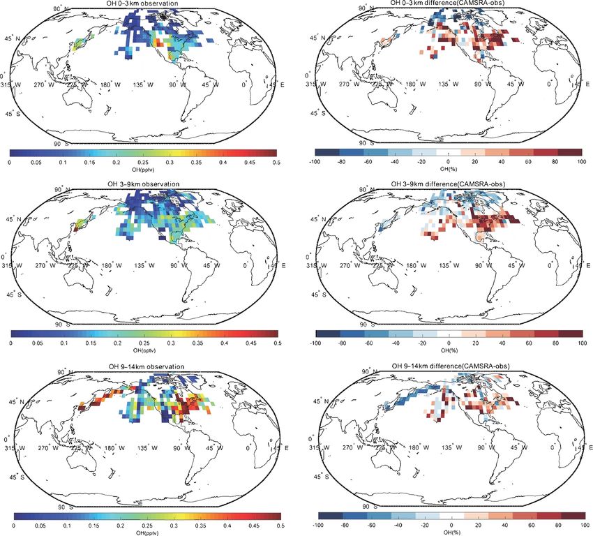
4500                            Y. Wang et al.: Evaluation of the CAMS global atmospheric trace gas reanalysis 2003–2016

Figure 3. Same as Fig. 2, but for the altitude bin of 3–9 km.

(positive in the Arctic and negative in the Southern Ocean),       there. In the middle troposphere, CIRA underestimates CO
with biases larger than 50 %. In this layer, the patterns of the   in most regions in the Northern Hemisphere, while it overes-
biases over the Pacific Ocean are different than in the lower      timates CO in the Southern Hemisphere. In the upper layer,
layers.                                                            the biases of CIRA are also large at high latitudes, but the
   CIRA agrees better with the observations than MACCRA.           biases are positive in the both polar regions.
In the low troposphere, the biases are smaller than those de-         The agreement between the CO measurements and the
rived with MACCRA, and the large negative biases in the            CAMSRA is generally good, with biases generally smaller
Arctic found in MACCRA disappear with CIRA. The mean               than 15 %. In the low and middle troposphere, the CAMSRA
bias of CIRA is only of the order of 10 %. CIRA underesti-         behaves similarly to CIRA; however, in the upper layer, the
mates the CO observation in the region of the northern Pa-         biases are different. The biases in CAMSRA become smaller
cific Ocean, but MACCRA overestimates the concentrations           in the polar region. CAMSRA underestimates CO concen-

Atmos. Chem. Phys., 20, 4493–4521, 2020                                            www.atmos-chem-phys.net/20/4493/2020/
Y. Wang et al.: Evaluation of the CAMS global atmospheric trace gas reanalysis 2003–2016                                4501

Figure 4. Same as Fig. 2, but for the altitude bin of 9–14 km.

trations in most regions of the low and middle latitudes, with   most regions except west of North America. The biases are
biases less than 20 %.                                           large in the polar stratosphere, where they reach about 50 %.
   The bias between the control run and the CO observa-             When confronted with CO data collected by airborne in-
tions is larger than for the CAMSRA. The bias pattern of         strumentation, all three reanalyses provide good results in
the control run in the lowest layer is similar to that of CAM-   the low and middle troposphere; however, the two early re-
SRA, but the positive biases in the Southern Hemisphere are      analyses are not successful when considering the field obser-
larger (about 30 %). In the free troposphere, the control run    vations made in the polar region, specifically in the upper
underestimates the CO concentration at latitudes north of        troposphere–lower stratosphere. The situation is improved
40◦ N, similar to the CAMSRA, but overestimates the CO           with the new CAMSRA reanalysis. The control simulations
elsewhere. The positive model biases in the Southern Hemi-       performed without assimilation overestimate the CO concen-
sphere and tropics are efficiently removed by the assimilation   tration in the Southern Hemisphere. The linear regression pa-
of CAMSRA. In the upper layer, the biases are positive in        rameters of CO are shown in Table 5. For all the data points,

www.atmos-chem-phys.net/20/4493/2020/                                            Atmos. Chem. Phys., 20, 4493–4521, 2020
4502 Y. Wang et al.: Evaluation of the CAMS global atmospheric trace gas reanalysis 2003–2016
Table 4. Linear regression of ozone between observations and models.
All data Troposphere data (> 350 hPa)
N MB MAE R2 Slope RMSE N MB MAE R2 Slope RMSE
MACCRA 19 522 0.59 13.01 0.9291 1.02 26.064 16 009 0.21 9.13 0.6145 0.71 11.705
CIRA 22 308 −1.87 12.71 0.9298 0.94 22.472 18 782 −2.95 9.58 0.6498 0.67 11.232
CIRA (2003–2012) 19 522 −1.18 12.67 0.9341 0.94 23.225 16 009 −2.29 8.99 0.6111 0.66 10.823
CAMSRA 22 308 1.92 11.90 0.9375 0.94 21.174 18 782 1.01 8.77 0.6927 0.72 10.996
CAMSRA (2003–2012) 19 522 2.49 11.97 0.9412 0.94 21.889 16 009 1.55 8.32 0.6608 0.72 10.608
Control 22 308 −3.89 13.46 0.8935 0.84 25.398 18 782 −1.68 9.18 0.6687 0.66 10.611
Control (2003–2012) 19 522 −3.71 13.72 0.8966 0.85 26.662 16 009 −1.08 8.76 0.6229 0.63 10.155
Note: N is the number of points considered for the calculation of the correlation, MB the mean bias (ppb), MAE the mean absolute error (ppb), R the correlation coefficient and RMSE
the root mean square error (ppb).
the correlations are weak due to the extreme values appear- in the higher levels are about 50 %. In the case of OH, the
ing in localized pollution plumes, which are not captured by calculated values are overestimated at middle and low lati-
coarse-resolution global models. After filtering out these ex- tudes, which may lead to a shorter lifetime of NO2 , consis-
treme values (values larger than 300 ppb), the correlations tent with the vertical distribution of NOx discussed above.
of CO between the observations and models improve sub- CAMSRA underestimates OH concentrations in the Arctic
stantially. The correlation calculated using CAMSRA is the region, which may be related to the overestimation of CO in
highest, with a correlation coefficient of 0.71 and a slope of that region. Finally, no clear pattern is found in the difference
0.78. The mean bias of CAMSRA is reduced with the assim- between model-simulated values and observations of HO2 .
ilation resulting from the correction of the positive bias in the
Southern Hemisphere.
5 Evaluation of vertical profiles at selected locations
4.3 Other chemical species
The CAMS reanalysis provides the global distribution of a
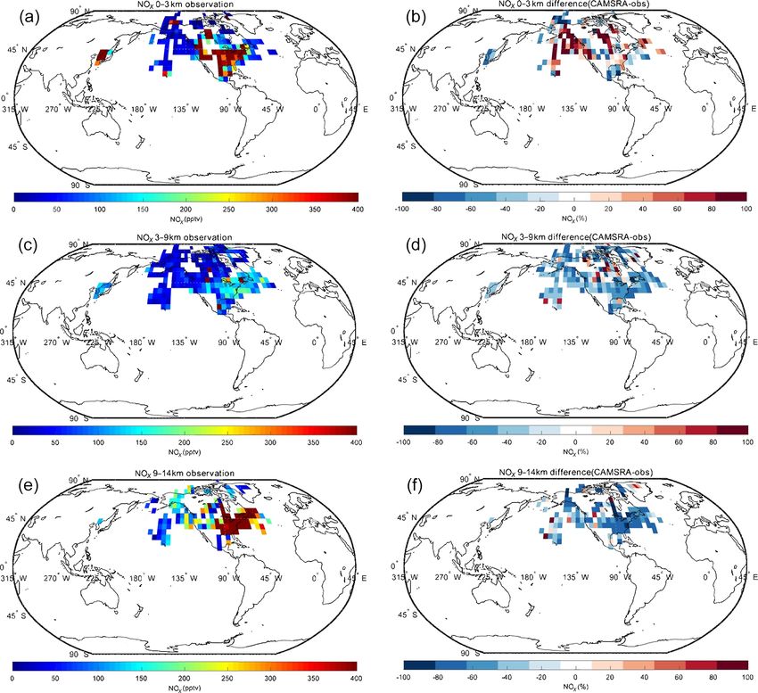
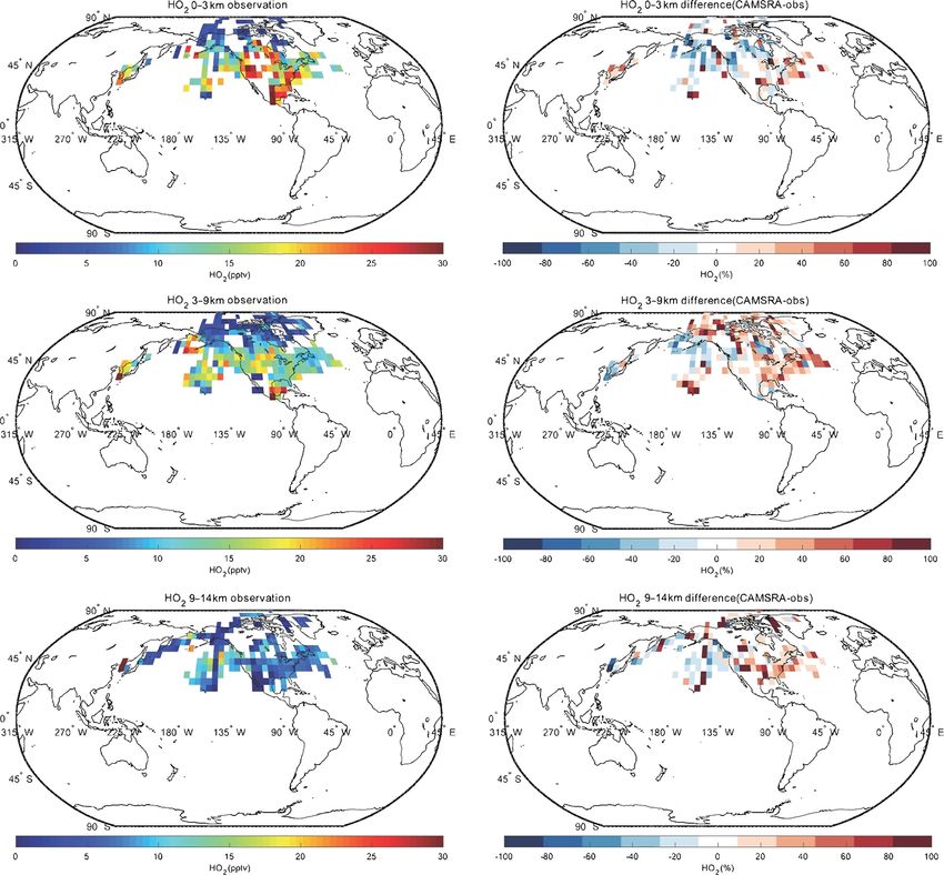
Spatial distributions of nitrogen oxides (NOx =NO + NO2 ), large number of chemical species that are not directly as-
the hydroxyl radical (OH), the hydroperoxyl radical (HO2 ) similated by the CAMS system but whose concentrations are
and formaldehyde (HCHO) for CAMSRA in the Northern calculated consistently with the assimilated species, ozone,
Hemisphere are provided in the Appendix. The CAMSRA carbon monoxide and nitrogen dioxide. We evaluate several
reanalysis values are compared with observations from air- key species calculated by CAMSRA at four selected loca-
craft for three different layers of the atmosphere. Because tions with observations from NASA campaigns (INTEX-A
the measurements of NOx , OH, HO2 and HCHO used in the in 2004, INTEX-B in 2006 and ARCTAS in 2008) that took
work are only in North America, the Arctic and Korea, the place with the DC-8 research aircraft (Fig. 8). These cam-
analyses below are for these regions. paigns provide information on the atmospheric abundance of
In the case of NOx , the CAMSRA reanalysis underes- several reactive gases related to ozone and CO chemistry.
timates the values measured in the middle and upper tro- The vertical profiles at the chosen locations are averaged
posphere but overestimates the observed values in the low- based on the ARCTAS campaign in the case of the Arctic
est layer. There are several possible reasons: (1) the model region (measurements north to 60◦ N), on the INTEX-B cam-
overestimates the effect of regional pollution sources; (2) the paign in the case of Hawaii and Mexico, and on INTEX-A in
model underestimates the local production (e.g., lightning); the case of the Bangor data. Since only O3 , CO and NO2 are
(3) the model underestimates the convective transport; (4) the assimilated in CAMSRA reanalysis, the control simulation
model underestimates the lifetime of the surface emissions. without assimilation is shown only for O3 , CO and NOx . A
We also compared the NOx fields produced by CAMSRA comparison between the reanalysis and the control simula-
and the control run in order to assess the benefit of NO2 as- tions for species other than O3 , CO and NOx is not shown
similation. Both fields are very similar, which suggests that because the differences between the two runs are very small.
the assimilation does not significantly improve the reanal- The vertical profiles of ozone, carbon monoxide, nitrogen ox-
ysis of NOx . This is explained by the fact that NO2 has a ides (NOx ), the hydroxyl (OH) and hydroperoxyl (HO2 ) rad-
short lifetime. Most of the impact of the data assimilation is ical, formaldehyde (HCHO), hydrogen peroxide (H2 O2 ), ni-
therefore lost between analysis cycles (Inness et al., 2015). tric acid (HNO3 ), peroxyacetyl nitrate (PAN), ethene (C2 H4 ),
In the case of HCHO, the reanalysis underestimates the ob- ethane (C2 H6 ), propane (C3 H8 ), methanol (CH3 OH), ace-
served concentrations at all levels. The negative biases in the tone (CH3 COCH3 ), methyl hydroperoxide (CH3 OOH), and
low troposphere are between 20 % and 40 %, while those ethanol (C2 H5 OH) are shown in Figs. 9, 10, 11 and 12.
Atmos. Chem. Phys., 20, 4493–4521, 2020 www.atmos-chem-phys.net/20/4493/2020/Y. Wang et al.: Evaluation of the CAMS global atmospheric trace gas reanalysis 2003–2016 4503
Figure 5. Campaign observations of CO (a). (b) The relative difference in percent between MACCRA and the observations (MACCRA –
observation). (c) The difference between CIRA and the observations (CIRA – observation). (d) The difference between CAMSRA and the
observations (CAMSRA – observation), and (e) the difference between the control run and the observation (control – observation). The data
are averaged to 5◦ × 5◦ (latitude × longitude) and to the altitude bin of 0–3 km.
We first examine the case of the three assimilated species. control run underestimates the O3 concentration above 1 km,
In general, the profiles calculated with assimilated observa- particularly above 6 km of altitude. The assimilation brings
tions are in good agreement with the profiles observed by air- the profile much closer to the aircraft data. The concentra-
borne instruments. There are some interesting points to note, tions calculated by the control and the reanalysis runs in the
however. surface layer below 1 km are almost twice as large as those
derived from the observations, which may be affected by the
5.1 Ozone halogen chemical removal in Arctic spring. In the free tropo-
sphere and low stratosphere, the agreement is best for CAM-
SRA. In Bangor (Fig. 10), the control and reanalysis simu-
In the case of ozone in the Arctic (Fig. 9), where the verti-
lations underestimate the aircraft observations in the upper
cal profile is strongly affected by stratospheric processes, the
www.atmos-chem-phys.net/20/4493/2020/ Atmos. Chem. Phys., 20, 4493–4521, 20204504 Y. Wang et al.: Evaluation of the CAMS global atmospheric trace gas reanalysis 2003–2016
Figure 6. Same as Fig. 5, but for the altitude bin of 3–9 km.
Table 5. Linear regression of CO between the aircraft campaign observations and the reanalyses.
All data Data < 300 ppb
N MB MAE R2 Slope RMSE N MB MAE R2 Slope RMSE
MACCRA 18 376 −10.40 27.13 0.2005 0.30 54.921 17 972 −5.96 18.69 0.5992 0.63 23.346
CIRA 21 353 −6.55 28.56 0.3990 0.49 60.912 20 254 −2.48 17.72 0.6775 0.72 25.052
CIRA (2003–2012) 18 376 −4.86 23.71 0.3573 0.42 51.397 17 894 −1.65 16.25 0.6588 0.70 22.900
CAMSRA 21 353 −6.85 29.23 0.3559 0.49 66.706 20 233 −3.82 17.34 0.7061 0.78 25.284
CAMSRA (2003–2012) 18 376 −5.42 25.26 0.2716 0.40 60.387 17 869 −3.21 16.04 0.6863 0.77 23.553
Control 21 353 −0.11 31.78 0.3565 0.50 68.489 20 187 2.45 20.15 0.6588 0.75 27.013
Control (2003–2012) 18 376 −0.25 27.74 0.2746 0.41 60.123 17 881 2.03 19.11 0.6234 0.71 24.920
Note: N is the number of points considered for the calculation of the correlation, MB the mean bias (ppb), MAE the mean absolute error (ppb), R the correlation coefficient and RMSE the
root mean square error (ppb).
Atmos. Chem. Phys., 20, 4493–4521, 2020 www.atmos-chem-phys.net/20/4493/2020/Y. Wang et al.: Evaluation of the CAMS global atmospheric trace gas reanalysis 2003–2016 4505 Figure 7. Same as Fig. 5, but for the altitude bin of 9–14 km. troposphere, while they overestimate the measurements near with assimilated ozone should be better constrained. This re- the surface. sult may be due to the fact that the constraint on tropospheric The low-latitude ozone profiles (Figs. 11 and 12) are well ozone is weak and the bias correction may be distributed in- reproduced by the reanalysis. However, the control run tends correctly in the vertical. In Mexico City, the model represents to overestimate ozone in Mexico City and to a lesser extent in the ozone bulge that is detected by the airborne instruments Hawaii. In this last region, the agreement of O3 between the at 2 to 3 km and is observed for most chemical species. At observations and models is quite good below 7 km: the bi- higher altitudes, the control model overestimates the ozone ases are positive and smaller than 10 %, which is opposite to concentration; however, the bias is reduced by the CAMSRA what is found in the Arctic. The reanalysis provides slightly assimilation. better results than the control run. At higher altitudes the pos- itive biases get larger and the CAMSRA data become worse than in the control run, which is surprising since the model www.atmos-chem-phys.net/20/4493/2020/ Atmos. Chem. Phys., 20, 4493–4521, 2020
4506                              Y. Wang et al.: Evaluation of the CAMS global atmospheric trace gas reanalysis 2003–2016

Table 6. Qualitative summary of the overestimation and underestimation by the CAMSRA for several observed chemicals at four geographic
locations and at two altitudes (6 km and the surface).

                                                        At 6 km                                                   surface
                                   Arctic      Bangor       Hawaii      Mexico City         Arctic     Bangor       Hawaii       Mexico City
                O3                 G           G            G           O                   OO         O            G            O
                CO                 G           U            G           U                   G          O            U            O
                NOx                UU          U            U           G                   U          OO           O            O
                OH                 UU          O            G           G                   UU         O            O            G
                HO2                O           O            G           O                   U          O            G            O
                H2 O2              UU          U            G           G                   UU         G            O            OO
                HNO3               UU          U            UU          G                   U          O            U            O
                PAN                U           U            O           OO                  O          OO           OO           OO
                C2 H4              U           G            UU          UU                  U          OO           O            G
                C2 H6              UU          UU           U           U                   UU         UU           UU           UU
                C3 H8              UU          UU           U           U                   UU         UU           UU           UU
                HCHO               UU          UU           U           U                   UU         U            G            O
                CH3 OH             UU          U            U           G                   O          O            G            OO
                CH3 COCH3          UU          UU           UU          UU                  UU         G            UU           U
                C2 H5 OH           UU          UU                       UU                  UU         O                         U
                CH3 OOH                        UU           U           U                              G            U            OO

              Note: G = −10 % < bias < 10 %; O = 10 % < bias < 40 %; U = −40 % < bias < −10 %; OO = bias > 40 %; UU = bias < −40 %.

                                                                                   the simulation significantly as MOPITT observations with
                                                                                   latitudes higher than 65◦ were excluded in the CAMS assim-
                                                                                   ilation. It increases the biases in troposphere CO in CAM-
                                                                                   SRA but decreases the positive biases in the stratosphere. In
                                                                                   Bangor (Fig. 10), both the control and the reanalysis sim-
                                                                                   ulations underestimate the observed concentrations by typ-
                                                                                   ically 10 ppb above 3 km of altitude but underestimate the
                                                                                   surface concentrations. At low latitudes (Hawaii and Mex-
                                                                                   ico; Figs. 11 and 12), the control simulation overestimates the
                                                                                   concentrations by about 10 ppb in the free troposphere, while
                                                                                   CAMSRA underestimates the values observed from the DC-
                                                                                   8 by 10 ppb. In Hawaii in the first 2 km above the surface,
                                                                                   the control run provides concentrations that are about 10 %
                                                                                   lower than the aircraft observation. In Mexico, the control
                                                                                   model provides surface values that are 30 % higher than the
                                                                                   observation. The bulge observed at 2–3 km of altitude is not
                                                                                   reproduced by the model.

Figure 8. The location of the four selected regions. The red,                      5.3     Nitrogen oxides
green, blue and magenta rectangles show the Arctic (ARCTAS,
April–July 2008), Hawaii (INTEX-B, March–May 2006), Mex-
ico (INTEX-B, March–May 2006) and Bangor (INTEX-A, July–                           In the Arctic (Fig. 9) the control run underestimates NOx ,
August 2004), respectively.                                                        especially above 8 km, i.e., in the layers strongly influenced
                                                                                   by the injection of stratospheric air. The assimilation pro-
                                                                                   cess does not substantially reduce the discrepancy, since
5.2    Carbon monoxide                                                             the CAMS model does not include a detailed representa-
                                                                                   tion of stratospheric chemistry and NOx in the stratosphere is
In the case of Arctic CO (Fig. 9), the general agreement be-                       strongly underestimated because of this. In Bangor (Fig. 10),
tween the control and reanalysis runs and the observed pro-                        the models underestimate NOx above 2 km as in the Arctic
file is very good. The control run, however, slightly underes-                     but overestimate NOx below 2 km. In the low-latitude regions
timates the CO concentration in the troposphere but overesti-                      (Mexico and Hawaii; Figs. 11 and 12), the calculated profiles
mates it in the stratosphere. The assimilation does not change                     are in rather good agreement with the observations, except

Atmos. Chem. Phys., 20, 4493–4521, 2020                                                                   www.atmos-chem-phys.net/20/4493/2020/
Y. Wang et al.: Evaluation of the CAMS global atmospheric trace gas reanalysis 2003–2016 4507 Figure 9. Averaged profiles of the trace constituents over the Arctic during the ARCTAS campaign from April to July 2008. The black lines are the observations, the red lines correspond to the CAMSRA reanalysis, and the blue lines are the control run (only shown for O3 , CO and NOx ). The error bars represent the standard deviation of the data and model. www.atmos-chem-phys.net/20/4493/2020/ Atmos. Chem. Phys., 20, 4493–4521, 2020
4508                            Y. Wang et al.: Evaluation of the CAMS global atmospheric trace gas reanalysis 2003–2016

Figure 10. Averaged profiles of the trace constituents over Bangor during the INTEX-A campaign from July to August 2004. The black lines
are the observations, the red lines correspond to the CAMSRA reanalysis, and the blue lines are the control run (only shown for O3 , CO and
NOx ). The error bars represent the standard deviation of the data and model.

Atmos. Chem. Phys., 20, 4493–4521, 2020                                                   www.atmos-chem-phys.net/20/4493/2020/
Y. Wang et al.: Evaluation of the CAMS global atmospheric trace gas reanalysis 2003–2016                                     4509

below 2 km, where the influence from local air pollution is         5.7   Peroxyacetyl nitrate (PAN)
not well captured by the control and reanalysis simulations.
In Hawaii, the model tends to slightly underestimate the ob-        The agreement between the calculated and observed PAN
servation. As in the Arctic, this underestimation is larger in      vertical profile is good in the Arctic (Fig. 9), even though
the case of the reanalysis. In all regions except the Arctic, the   the concentrations are slightly underestimated between 2
models provide higher surface concentrations than suggested         and 8 km of altitude. The agreement is also good in Hawaii
by the measurements.                                                (Fig. 11) below 5 km of altitude, but a discrepancy of about
                                                                    50 % is found above this height. In Bangor (Fig. 10), PAN
5.4   Hydroxyl and hydroperoxyl radicals                            concentrations are overestimated by about 25 % in the free
                                                                    troposphere and by as much as a factor of 2 below 3 km of
In the Arctic (Fig. 9), the model underestimates OH con-            altitude. The calculated concentrations are slightly too high
centrations by about 0.02 ppt at all altitudes (of the order of     in Mexico City (Fig. 12). The model shows the presence of
50 %), which may be linked to the slight overestimation of          a peak in the PAN concentration at 3 km, but the calculated
calculated stratospheric CO. In the reanalysis, the concen-         concentration values are somewhat too low.
trations of HO2 are overestimated by about 1 pptv between
4 and 8 km of altitude. In Bangor (Fig. 10), the reanalysis         5.8   Primary organic compounds: ethene (C2 H4 ),
overestimates OH by about 0.2 pptv, which is coincident with              ethane (C2 H6 ) and propane (C3 H8 )
the underestimation of the CO concentration at this location.
The HO2 concentrations are overestimated by 3–5 pptv. In            In most cases, the model underestimates the measured con-
Hawaii, the simulations made for the reanalysis overestimate        centrations of the primary hydrocarbons, which indicates that
the OH concentrations below 6 km but underestimate them             the emissions are too low. The discrepancy is substantial at
above 8 km, which is consistent with the overestimation of          all altitudes, for example for C2 H4 in Hawaii (Fig. 11), as
high-altitude CO in the control run. In Mexico City, the sim-       well as C3 H8 in the Arctic (Fig. 9) and in Bangor (Fig. 10).
ulated OH concentrations are larger than the measurements           Calculated C2 H6 is substantially lower than suggested by the
below 8 km but smaller above 8 km. The reanalysis overesti-         observations at all four locations. In Mexico City (Fig. 12),
mates HO2 by about 4 pptv or 20 %.                                  the model rather successfully reproduces the vertical profile
                                                                    of C2 H4 but underestimates C3 H8 below 5 km of altitude.
5.5   Hydrogen peroxide                                             This last compound is well represented in Hawaii in the up-
                                                                    per troposphere but is underestimated by the model below
In the Arctic (Fig. 9), where the calculated concentrations         7 km.
of HO2 are too high in CAMSRA, the concentration of hy-
drogen peroxide is overestimated by typically a factor of 2.        5.9   Secondary organic compounds: formaldehyde
In Bangor (Fig. 10), the overestimation is of the order of                (HCHO), methanol (CH3 OH), acetone
20 %. The agreement between the reanalysis and observa-                   (CH3 COCH3 ), ethanol (C2 H5 OH) and methyl
tions is generally good in Hawaii (Fig. 11) and Mexico City               hydroperoxide (CH3 OOH)
(Fig. 12), except in the lower levels of the atmosphere, where
the model overestimates the concentrations.                         As should be expected from the underestimation by the re-
                                                                    analysis of the atmospheric concentration of the primary hy-
5.6   Nitric acid                                                   drocarbons, the model also underestimates the abundance
                                                                    of oxygenated organic species in the troposphere. This is
Nitric acid concentrations are strongly affected by wet scav-       the case in the Arctic (Fig. 9), where the abundances of
enging in the troposphere and, at high latitudes, by the down-      formaldehyde, acetone and ethanol are underestimated by
ward flux of stratospheric air (Murphy and Fahey, 1994; We-         typically factors of 3 to 8. Methanol is too low by about 30 %.
spes et al., 2007). The reanalysis generally underestimates         Large discrepancies are also found in Bangor (Fig. 10) where
the concentration of HNO3 above 2 km of altitude. This is           methanol and acetone are underestimated by a factor of 2 and
the case in the Arctic (Fig. 9), Bangor (Fig. 10) and Hawaii        methyl peroxide by a factor of 5. In Hawaii (Fig. 11), the con-
(Fig. 11). The discrepancy is particularly large in the upper       centration of formaldehyde is slightly underestimated in the
levels of the Arctic, which implies that (1) scavenging of          middle and upper troposphere, but the discrepancy reaches a
HNO3 is too strong, and (2) the reactive nitrogen (e.g., NOx )      factor of 2 at 2 km of altitude. Methanol is underestimated by
in the stratosphere is too low due to missing stratospheric         30 %, but acetone and ethanol are underestimated by a factor
chemistry. The model accounts for the high concentrations           of 2. The model is in better agreement with the observations
observed in the lowest levels of the atmosphere, specifically       in Mexico City (Fig. 12): this is the case for formaldehyde
in Mexico City (Fig. 12) and to a lesser extent in Bangor and       (except below 4 km where the calculated concentrations are
Hawaii.                                                             a factor of 3 too low), methanol (except at the surface) and

www.atmos-chem-phys.net/20/4493/2020/                                                Atmos. Chem. Phys., 20, 4493–4521, 2020
4510 Y. Wang et al.: Evaluation of the CAMS global atmospheric trace gas reanalysis 2003–2016 Figure 11. Averaged profiles of the trace constituents over Hawaii during the INTEX-B campaign from March to May 2006. The black lines are the observations, the red lines correspond to the CAMSRA reanalysis, and the blue lines are the control run (only shown for O3 , CO and NOx ). The error bars represent the standard deviation of the data and model. Atmos. Chem. Phys., 20, 4493–4521, 2020 www.atmos-chem-phys.net/20/4493/2020/
Y. Wang et al.: Evaluation of the CAMS global atmospheric trace gas reanalysis 2003–2016                                             4511

Figure 12. Averaged profiles of the trace constituents over Mexico during the INTEX-B campaign from March to May 2006. The black lines
are the observations, the red lines correspond to the CAMSRA reanalysis, and the blue lines are the control run (only shown for O3 , CO and
NOx ). The error bars represent the standard deviation of the data and model.

www.atmos-chem-phys.net/20/4493/2020/                                                     Atmos. Chem. Phys., 20, 4493–4521, 2020
4512                          Y. Wang et al.: Evaluation of the CAMS global atmospheric trace gas reanalysis 2003–2016

methyl hydroperoxide except below 4 km. Ethanol is under-            In the Arctic, the ratio derived from observations (typically
estimated by a factor of 2.                                       equal to 1; see the black curve in Fig. 13) is about a factor of
   To summarize the discussion, we have qualified the de-         2 smaller than the calculated ratio between 6 and 10 km of
gree of success of the reanalysis model versus the observa-       altitude. In Bangor, its value (about 2 to 3) is higher than the
tional vertical profiles in the four regions of the world that    model calculations. Perhaps the most interesting point is the
are considered in the present study. The results, based on a      substantial discrepancy between the models and the obser-
subjective comparison between the vertical profiles derived       vations in the upper troposphere of the tropics (Hawaii and
from the CAMSRA and the profiles measured independently           Mexico). One notes, for example, that the observed ratio does
by airborne instruments, are presented in Table 6 for the al-     not increase as expected from theory, and at 11 km, for exam-
titudes of 6 km above the ground and at the Earth’s surface,      ple, the calculated ratio of close to 1 when derived from the
respectively. The symbols used in this table are the following:   observations reaches a value of the order of 4 or 5. Among
G for good agreement (bias < 10 %), O for overestimation by       possible causes for this discrepancy is an underestimation
the reanalysis model (10 % < bias < 40 %) and U for underes-      of the correction factor X due to reactions not considered
timation (−40 % < bias < −10 %). Double symbols (i.e., OO         in the models. Possible mechanisms include the reactions of
or UU) indicate from a subjective analysis that the disagree-     NO with the methyl peroxy radical (CH3 O2 ) and with BrO
ment is large (bias > 40 %).                                      (Sasha Madronich, personal communication, 2019). CH3 O2
                                                                  plays a significant role in the NO to NO2 conversion. The
5.10   Concentration ratios                                       BrO radical is expected to affect the NO to NO2 ratio if the
                                                                  BrO concentration becomes larger than 2–5 pptv. Another
In order to analyze the performance of the reanalysis and to      point to stress is the large uncertainty that results from di-
reproduce the observed relationships between different react-     viding two mean concentration values to which substantial
ing species, we present and discuss the vertical distribution     uncertainties are attached so that the stated ratio derived from
of the concentration ratio between photochemically coupled        mean observations may be subject to a large error.
chemical compounds. In order to avoid the chemically and             Figure 13 also shows the concentration ratio between PAN
dynamically complex situation encountered in the boundary         and NO2 and between HNO3 and NO2 . In the first case, the
layer, we limit this analysis to results (models and observa-     ratios derived from the models (control run and reanalysis)
tions) obtained above 4 km of altitude. We focus here on the      are in fair agreement with the ratios derived from the mea-
NO/NO2 , PAN/NO2 , HNO3 /NO2 and HO2 /OH concentra-               surements of NO2 and PAN concentrations. The ratio de-
tion ratios (Fig. 13).                                            creases with height in the Arctic and Bangor but is relatively
   We first examine for the four locations considered in          constant with height (typically 10–20), with some elevated
the present study (Arctic, Bangor, Hawaii and Mexico) the         values at some specific altitudes. In the case of the HNO2 to
NO/NO2 concentration ratios derived from the aircraft ob-         NO2 ratio, the differences between ratios derived from the
servations of NO and NO2 , respectively, as well as the simi-     models and the aircraft observations can be substantial. The
lar ratios produced by the control case (blue curves), reanal-    control and reanalysis runs (blue and red curves) underesti-
ysis models (red curves) or derived from an approximative         mate the ratio in the Arctic and in Bangor. The agreement
expression based on the photochemical theory of the tropo-        is somewhat better in Hawaii and in Mexico, even though
sphere (green curves). We note at all locations that the value    large differences exist at specific altitudes. These discrep-
derived from the reanalysis (with a detailed chemical scheme      ancies can probably be explained by the role played by the
included) is in good agreement with the value derived from        heterogeneous conversion of nitrogen oxides to nitric acid,
the simple photostationary expression:                            which depends on the chaotic behavior of clouds and aerosols
 [NO]            JNO2                                             in the troposphere. The green curve provides an estimate of
      =                         ,                                 the ratio derived from the following expression (assuming
[NO2 ] k1 [O3 ] + k2 [HO2 } + X
                                                                  equilibrium) that ignores any heterogeneous conversion but
where JNO2 (about 10−2 s−1 in the entire troposphere for          is calculated using the observed values of OH:
a solar zenith angle of 45◦ ) represents the photolysis co-
efficient of NO2 , and k1 and k2 are the rate constants of        [HNO3 ]       k3 [OH]
                                                                          =                 .
the reaction of NO with ozone and the hydroperoxy radical          [NO2 ]   JHNO3 + k4 [OH]
(HO2 ), respectively (Burkholder et al., 2015). The symbol
X accounts for the effects of additional conversion mech-         Here, JHNO3 (about 6 × 10⁻⁷ s) is the photolysis coefficient
anisms of NO to NO2 . Note that, as the temperature and           for nitric acid, while k3 and k4 are the kinetic coefficients for
the ozone number density decrease with height in the tro-         the reactions between NO2 and OH and between HNO3 and
posphere, the NO/NO2 ratio tends to increase with altitude.       OH, respectively (Burkholder et al., 2015).
In the lower stratosphere, the ratio is expected to decrease as      Finally, we show in Fig. 13 the concentration ratio between
the ozone concentration rapidly increases with height above       HO2 and OH, which is influenced by carbon monoxide, ni-
the tropopause.                                                   tric oxide and ozone that, to a good approximation, can be

Atmos. Chem. Phys., 20, 4493–4521, 2020                                            www.atmos-chem-phys.net/20/4493/2020/
You can also read