Crop-specific exposure to extreme temperature and moisture for the globe for the last half century
←
→
Page content transcription
If your browser does not render page correctly, please read the page content below
LETTER • OPEN ACCESS

Crop-specific exposure to extreme temperature and moisture for the
globe for the last half century
To cite this article: Nicole D Jackson et al 2021 Environ. Res. Lett. 16 064006

View the article online for updates and enhancements.

                              This content was downloaded from IP address 192.80.105.156 on 20/05/2021 at 22:42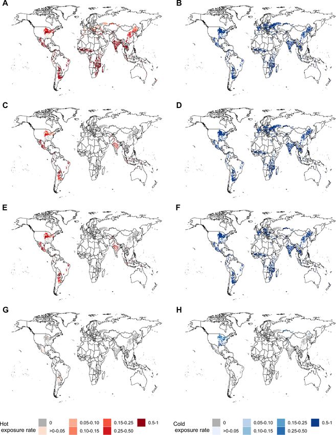
Environ. Res. Lett. 16 (2021) 064006 https://doi.org/10.1088/1748-9326/abf8e0
LETTER
Crop-specific exposure to extreme temperature and moisture for
OPEN ACCESS
the globe for the last half century
RECEIVED
14 December 2020 Nicole D Jackson1, Megan Konar1, Peter Debaere2 and Justin Sheffield3
REVISED 1
17 March 2021 Department of Civil and Environmental Engineering, University of Illinois at Urbana-Champaign, Urbana, IL 61821,
United States of America
ACCEPTED FOR PUBLICATION 2
Darden School of Business, University of Virginia, Charlottesville, VA 22903, United States of America
16 April 2021 3
Geography and Environmental Science, University of Southampton, Southampton, United Kingdom
PUBLISHED
17 May 2021 E-mail: mkonar@illinois.edu
Keywords: crop-specific, weather extremes, temperature, moisture, global, gridded, time series
Original Content from
this work may be used Supplementary material for this article is available online
under the terms of the
Creative Commons
Attribution 4.0 licence.
Any further distribution Abstract
of this work must
maintain attribution to
Global assessments of climate extremes typically do not account for the unique characteristics of
the author(s) and the title individual crops. A consistent definition of the exposure of specific crops to extreme weather
of the work, journal
citation and DOI. would enable agriculturally-relevant hazard quantification. To this end, we develop a database of
both the temperature and moisture extremes facing individual crops by explicitly accounting for
crop characteristics. To do this, we collate crop-specific temperature and moisture parameters from
the agronomy literature, which are then combined with time-varying crop locations and
high-resolution climate information to quantify crop-specific exposure to extreme weather.
Specifically, we estimate crop-specific temperature and moisture shocks during the growing season
for a 0.25◦ spatial grid and daily time scale from 1961 to 2014 globally. We call this the
Agriculturally-Relevant Exposure to Shocks (ARES) model and make all ARES output available
with this paper. Our crop-specific approach leads to a smaller average value of the exposure rate
and spatial extent than does a crop-agnostic approach. Of the 17 crops included in this study, 13
had an increase in exposure to extreme heat, while 9 were more exposed to extreme cold over the
past half century. All crops in this study show a statistically significant increase in exposure to both
extreme wetness and dryness. Cassava, sunflowers, soybeans, and oats had the greatest increase in
hot, cold, dry, and wet exposure, respectively. We compare ARES model results with the EM-DAT
disaster database. Our results highlight the importance of crop-specific characteristics in defining
weather shocks in agriculture.
1. Introduction definition of crop-specific exposure to extreme tem-
perature (e.g. too hot and too cold) and moisture (e.g.
Extreme weather (also called ‘shocks’ and ‘hazards’) too wet and too dry) and consistently evaluate its spa-
negatively impacts agricultural yield and total factor tial and temporal trends at the global scale for the past
productivity [1–7]. Weather shocks are projected to half century.
increase in both frequency and severity in the future Prior work has evaluated extreme weather in
[8, 9], making it important to better understand agriculture [14, 15]. It is increasingly being recog-
the relationship between extreme weather and agri- nized that crops have distinct physiological thresholds
culture. In recent years, there has been a dramatic that lead them to be impacted differently by the
increase in research to evaluate extreme weather in same weather. This means that some crops are more
agriculture [10–13]. However, there is still a need sensitive than others [16, 17]. For example, corn
for a historical assessment of extreme weather that yields were shown to increase with temperature
accounts for the characteristics of specific crops and up to 29◦ C in the United States, while soy has a
includes both temperature and moisture extremes. higher threshold of 30◦ C and cotton has an even
The goal of this paper is to develop a consistent higher threshold of 32◦ C [18]. Yet, most work to
© 2021 The Author(s). Published by IOP Publishing Ltd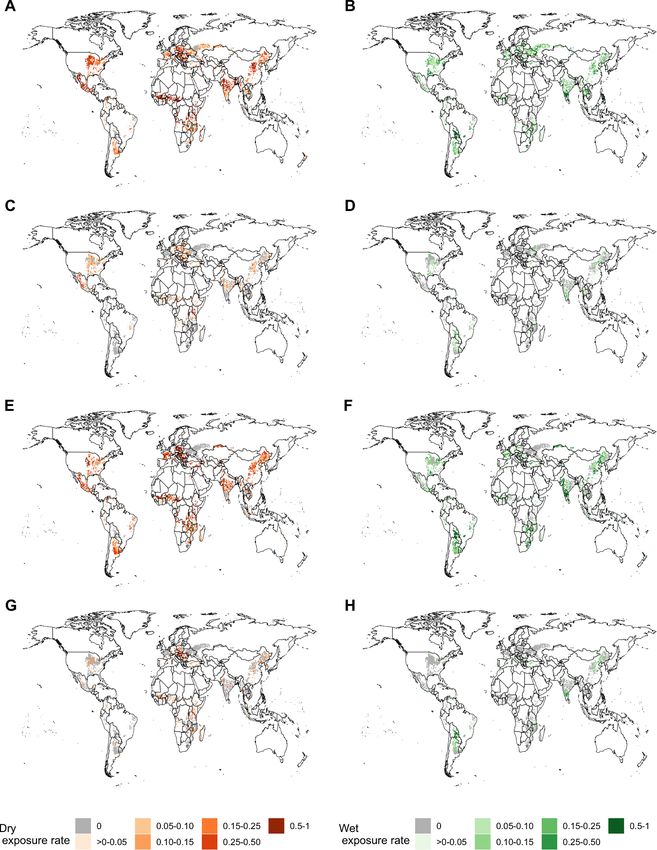
Environ. Res. Lett. 16 (2021) 064006                                                                      N D Jackson et al

quantify weather extremes in agriculture has been              Table 1. Summary of gridded datasets used in this study.
agnostic to crop type, particularly in terms of mois-      Source       Spatial scale Time period Variable collected
ture demands [12, 19]. Studies that do distinguish by
crop type typically focus on specific regions of the       Sheffield    0.25◦        1961–2014       Daily maximum
world, rather than considering the entire globe [18],      et al [32]                                temperature,
                                                                                                     minimum
or a small number of crops [10, 17, 20]. Likewise,
                                                                                                     temperature,
extremes occur at both tails of the distribution [20–                                                precipitation
23], making it important to evaluate exposure to tem-                                                and reference
peratures that are both too hot and too cold, as well                                                evapotranspiration
as moisture stress from soil that is too wet and too       Jackson      0.5◦         1961–2014       Probabilistic
dry [11, 24]. However, many studies focus on a single      et al [29]                                estimates of crop-
tail of the distribution, such as drought [15, 25, 26]                                               specific areas
                                                           Sacks et al 5 arc min     2000            Primary and
or extreme heat [16, 27]. There is thus a need to
                                                           [34]                                      secondary crop
develop a crop-specific definition of climate extremes                                               calendars
and evaluate it for a comprehensive range of loca-
tions, times, extremes, and crops.
     A consistent definition of crop-specific climate      to climate extremes. To determine where specific
extremes would enable a retrospective analysis of how      crops are located in each year of the study, we use
these events have changed over time. This approach         PCAM [29]. We develop the Agriculturally-Relevant
would improve upon the Emergency Events Database           Exposure to Shocks (ARES) model to estimate crop-
(EM-DAT), which many studies that seek to examine          specific exposure to extreme weather. We use ARES
the relationship between extreme weather and agri-         to quantify historical exposure to extreme temper-
culture rely upon [11]. EM-DAT is a country-level          ature (too hot and too cold) and moisture (too wet
self-reported database of extreme events. However,         and too dry) by crop for 17 crops for the globe from
the fact that EM-DAT is self-reported is problem-          1961 to 2014. This enables us to ask the following
atic, because some countries may be more likely to         scientific questions: (a) How does our understand-
report extreme events in agriculture than others, lead-    ing of extreme weather in agriculture change with a
ing to bias in the dataset. Additionally, EM-DAT has       crop-specific approach? (b) How has the exposure of
broad representation of disasters, but was not spe-        certain crops to extreme weather changed over time?
cifically designed to represent the unique features of     (c) What is the spatial distribution of weather shocks
agricultural extremes. EM-DAT also reports events          around the world?
with significant economic impact rather than consist-
ently defined occurrence of hazards. This makes it dif-
                                                           2. Methods
ficult to compare climate hazards in agriculture across
                                                           We develop the ARES model to consistently evalu-
countries and through time using the EM-DAT data-
                                                           ate the evolution of extreme events to specific crops.
base. For this reason, the goal of this paper is to con-
                                                           ARES is built by integrating multiple data sources
sistently define agricultural extremes by crop across
                                                           (see table 1). In general, our approach begins with
space and time.
                                                           global gridded climate data that is winnowed by
     Prior work to determine the interaction between
                                                           crop-specific agronomic thresholds to identify crop-
weather and agriculture has been hampered by a
                                                           specific thermal and hydrologic extreme events in
coarse understanding of where crops are grown. At
                                                           time and space. Figure 1 provides an overview of our
the country spatial scale, time series information on
                                                           model framework. The ARES approach presents a
the locations of specific crops is available from the
                                                           consistent shock definition that is used to quantify
Food and Agriculture Organization. However, for
                                                           crop-specific exposure to extreme events as a time-
gridded land cover, many studies rely on estimates of
                                                           varying, gridded product. The following subsections
crop locations circa 2000 (e.g. as provided by [28])
                                                           provide details on the data sources, event construc-
with time-varying climate information [25]. These
                                                           tion, model assessment, and critical assumptions.
approaches would likely be improved by including
time-varying estimates of gridded crop locations. To       2.1. Data sources and integration
this end, we incorporate annual crop location maps         ARES is based upon multiple global gridded data-
from the Probabilistic Cropland Allocation Model           sets as well as crop-specific agronomic informa-
(PCAM) [29]. PCAM gridded crop maps are available          tion. Table 1 summarizes the global gridded data
at the annual time step from 1960 to 2014.                 products used in this study. We collate information
     In this study, we define crop-specific exposure       on crop-specific temperature thresholds in table 2.
to climate shocks. To do this, we draw upon the            Tmin represents the minimum temperature beyond
agronomy literature and collate crop parameters for        which the yield of that crop will decline; Tmax indic-
critical temperatures and moisture demands. We             ates the maximum temperature beyond which yield
fuse these agronomic parameters with detailed cli-         declines will occur. Topt shows the optimum temper-
mate information to define crop-specific exposure          ature for crop growth. Three critical temperatures are

                                              2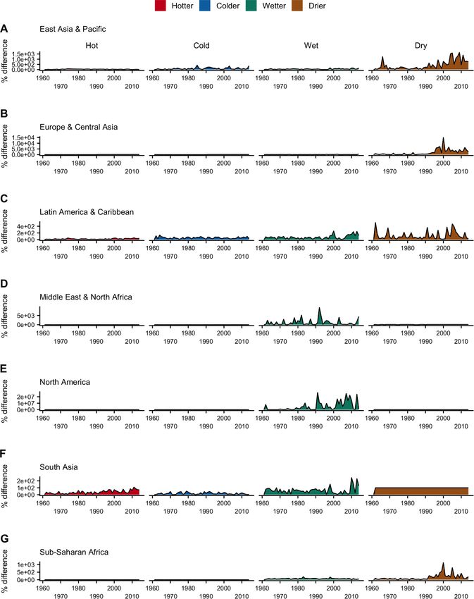
Environ. Res. Lett. 16 (2021) 064006                                                                           N D Jackson et al

   Figure 1. Schematic of the ARES methodology. Tmax refers to maximum temperature, Tmin is minimum temperature, ET0 is
   reference evapotranspiration, and P is precipitation.

determined for each crop in this study: minimum,                 the same threshold we averaged the values to obtain
optimum, and maximum. These thresholds were col-                 the threshold presented in table 2. We provide the
lected from dozens of research articles through a                full citation list for the agronomic research that
literature review that builds on previous efforts by             we drew from in the supporting information (SI)
Porter and Gawith [30], as well as Hatfield and                  (available online at stacks.iop.org/ERL/16/064006/
Prueger [31]. When multiple values were found for                mmedia).

                                                   3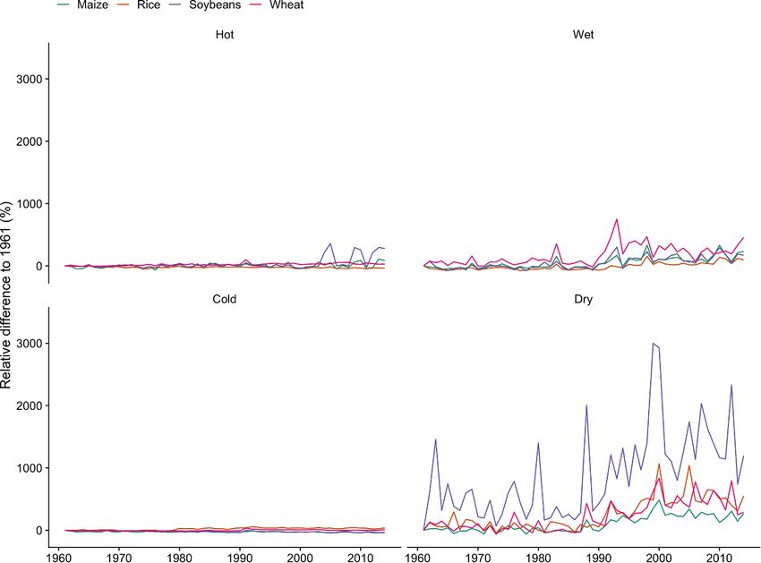
Environ. Res. Lett. 16 (2021) 064006                                                                                      N D Jackson et al

Table 2. Physiological crop thresholds and coefficients applied in this study. The crop coefficients are adapted from Doorenboos and
Pruitt [36] for the initial (ini), middle (mid), and endpoints (end) of the growing season. Seasons are identified as ‘M’ for main, ‘S’ for
secondary, and ‘W’ for winter.

                                                                  Thermal threshold (◦ C)                       Crop coefficient
Crop                Species                      Season         Tmin          Topt        Tmax           kini          kmid           kend

Barley              Hordeum vulgare              M              0.7          18.3         33.1           0.3           1.15           0.25
Barley                                           W            −12.0          11.5         33.0           0.3           1.15           0.25
Cassava             Manihot esculenta            M             15.0          27.0         45.0           0.3           0.95           0.725
Groundnuts          Arachis hypogaea             M             13.1          27.0         40.5           0.4           1.15           0.6
Maize               Zea mays                     M              6.2          30.8         42.0           0.3           1.2            0.475
Maize                                            S              6.2          30.8         42.0           0.3           1.2            0.475
Millet              Panicum miliaceum            M             10.7          32.5         43.8           0.3           1              0.3
Oats                Avena sativa                 M             −3.9          17.8         23.0           0.3           1.15           0.25
Oats                                             W             −4.8          11.3         23.0           0.3           1.15           0.25
Potato              Solanum tuberosum            M             −3.7          15.1         27.0           0.5           1.15           0.75
Rapeseed            Brassica napus               W              3.8          20.9         28.3           0.35          1.075          0.35
Rice                Oryza sativa                 M             13.5          27.6         35.4           1.05          1.2            0.75
Rice                                             S             13.5          27.6         35.4           1.05          1.2            0.75
Rye                 Secale cereale               W             −5.4          12.5         30.0           0.3           1.15           0.4
Sorghum             Sorghum bicolor              M              9.5          31.0         36.9           0.3           1.05           0.55
Sorghum                                          S              9.5          31.0         36.9           0.3           1.05           0.55
Soybeans            Glycine max                  M             11.4          28.3         39.4           0.4           1.15           0.5
Sugarbeet           Beta vulgaris                M             −1.6          20.3         32.8           0.35          1.2            0.7
Sunflowers          Helianthus annuus            M              7.4          29.4         43.1           0.35          1.075          0.35
Sweet Potato        Ipomoea batatas              M             14.9          28.9         40.0           0.5           1.15           0.65
Wheat               Triticum aestivum            M              6.4          21.6         28.7           0.3           1.15           0.325
Wheat                                            W              1.0          14.3         28.5           0.55          1.15           0.325
Yams                Dioscorea alata              M             14.8          25.2         37.4           0.5           1.1            0.95

    We obtain an update to the Princeton Global Met-                    averaged the lengths across all regions for each crop
eorological Forcing dataset [32, 33] for the period                     and use proportionality to assign agriculture calendar
1961–2014 for the following climate variables: max-                     days to each growth stage. This enables us to apply
imum temperature (Tmax ), minimum temperature                           crop coefficients from Doorenbos and Pruitt [36]
(Tmin ), precipitation (P), and reference evapotran-                    that vary by growth stage to the correct days within
spiration (ET0 ). These variables enable us to calculate                the agriculture calendar of each crop. Crop coeffi-
extremes in both temperature and moisture condi-                        cients for the development growth stage are estimated
tions. Note that these variables are obtained at the                    by averaging coefficients for the initial and middle
0.25◦ spatial resolution and daily time-step.                           stages. Similarly, the late growth stage coefficients are
    Global gridded crop calendars are obtained                          averages of the middle and endpoint coefficients.
from Sacks et al [34] at the 5 arcmin spatial resolution.                   We obtain crop-specific locations from the Prob-
The data is interpolated to a 0.25◦ spatial resolution                  abilistic Cropland Allocation Model (PCAM) [29] for
to match the climate data. These calendars provide us                   the period 1961–2014 at 0.5◦ spatial resolution. We
with information on which Julian day planting, grow-                    downscale PCAM data to 0.25◦ spatial resolution to
ing, and harvesting periods have started and ended.                     match the climate data. Each pixel’s unique latitude-
We treat the period from the end of planting to the                     longitude pairing allows us to construct annual crop-
start of harvesting as the growing season. A binary                     specific panels that integrate climate, crop calendar,
indicator is used to identify whether or not a given                    and land use data.
day occurs during the agricultural calendar. Note
                                                                        2.2. Thermal event exposure
that Sacks et al [34] provide information on multiple
                                                                        We quantify both extreme cold and hot temperat-
growing seasons for certain crops when applicable
                                                                        ure events annually. We do this by tracing through a
(see table 2), which we include in this study. Distinct
                                                                        series of phases to derive crop-specific thermal event
growing seasons are treated independently (e.g. the
                                                                        exposure rates (see figure 1). The goal is to win-
extreme events that occur in each growing season are
                                                                        now the database from generic (e.g. not crop-specific)
tabulated individually). Annual extreme event values
                                                                        thresholds to crop-specific extremes that occur only
for crops with multiple growing seasons are summed
                                                                        during the growing season. The approach is based on
across all growing seasons.
                                                                        a modification of the process developed by Teixeira
    It is particularly important to refine crop growth
                                                                        et al [27] and is summarized as follows:
phases to assess moisture extremes in crop pro-
duction. The length of each crop’s growth stages                        • Phase T1: restrict climate data to a generic optimal
is obtained from Doorenbos and Pruitt [35]. We                            threshold

                                                          4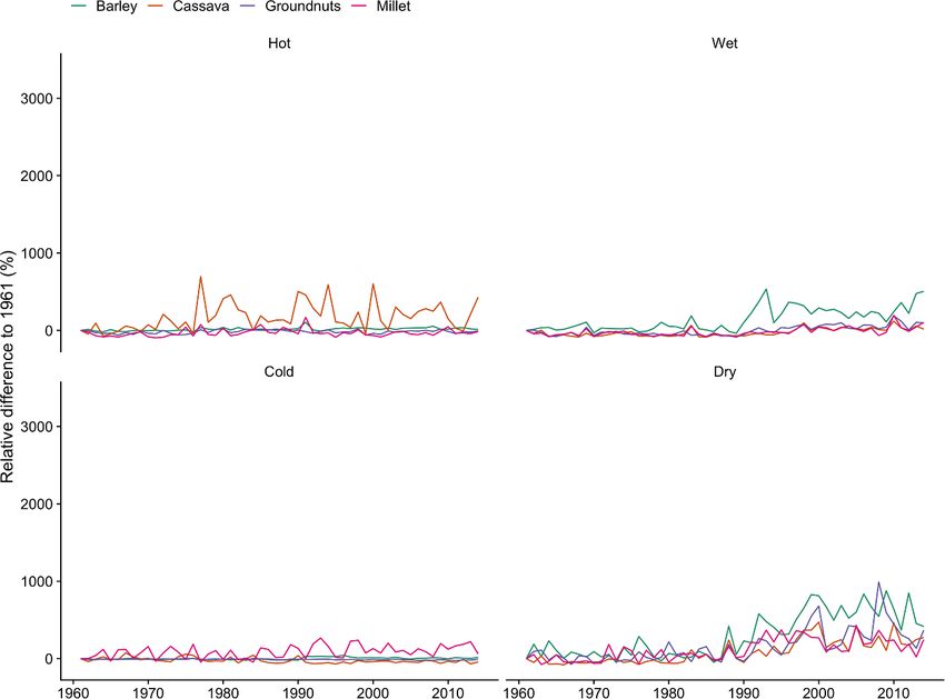
Environ. Res. Lett. 16 (2021) 064006 N D Jackson et al
• Phase T2: restrict climate data to the crop-specific 20.88 ◦ C for main, secondary, and winter seasons,
optimum threshold respectively.
• Phase T3: restrict climate data in time by crop cal- Phase T2: restrict climate data to the crop-specific
endars optimum threshold. The threshold for phase T2 is the
• Phase T4: restrict climate data with crop-specific crop-specific optimum temperature (Topt,crop,season )
extreme threshold for the given season (see table 2). Equation (2)
• Phase T5: repeat phases 1–4 for all crops, seasons, presents the binary specification for this phase,
and years in the study domain fT2,p,d,y,crop :
Throughout the phases, we use the daily maximum
1, if Tmax,p,d,y > Topt,crop,season
and minimum temperatures as it is consistent with fT2,p,d,y,crop = 1, if Tmin,p,d,y < Topt,crop,season (2)
approaches used by Zhu and Troy [12], Lobell et al
0, otherwise
[37], and Barlow et al [38]. The following are addi-
tional details on each of the thermal event phases: Phase T3: restrict climate data in time by crop
Phase T1: restrict climate data to a generic calendars. The calendar dataset from Sacks et al
optimum threshold. The threshold for phase T1 [34] provides crop- and season-specific, pixel-level
is based on a generic value across all crops per information on the first day of planting (dp,crop,PS )
season. The generic optimum is equal to the min- through the last day of harvest (dp,crop,HE ). These date
imum seasonal optimal value for maximum tem- ranges are used for each year (y) of the study domain.
perature events, and the maximum optimal value Equation (3) presents the binary specification for this
for minimum temperature events (see table 2 and phase, fT3,p,d,y,crop . Note that there is both a temperature
equation (1)). Equation (1) presents the sample bin- requirement and time requirement in this specifica-
ary indicator to identify events at the generic thermal tion that must be met on each day (d) in the year (y)
threshold: for the given pixel (p) and crop
{
1, if Tmax,p,d,y > min(Topt,crop,season ) 1, fT2 = 1 & dp,crop,PS ≤ d ≤ dp,crop,HE
fT3,p,d,y,crop =
fT1,p,d,y,crop = 1, if Tmin,p,d,y < max(Topt,crop,season ) 0, otherwise
0, otherwise (3)
(1)
where PS is plant start date and HE is harvest end.
where fT1,p,d,y,crop is the resulting binary indicator for Phase T4: restrict climate data to the crop-
phase T1 at pixel p, Tmax,p,d,y is the pixel p’s maximum specific extreme threshold (i.e. the minimum and
temperature on day d for year y, Tmin,p,d,y is pixel maximum values provided in table 2). For max-
p’s daily minimum temperature, and Topt,crop,season imum temperature events, the thermal threshold
are the crop- and season-specific optimum temperat- is equivalent to the crop-specific maximum tem-
ures presented in table 2. The minimum optimal val- perature. For minimum temperature events, the
ues for maximum temperature are 15.05 ◦ C, 27.6 ◦ C, extreme threshold is the minimum of the frost tem-
and 11.25 ◦ C for main, secondary, and winter sea- perature (0 ◦ C) and the crop- and season-specific
sons, respectively. The maximum optimal values for minimum temperature. Equation (4) presents the
minimum temperature are 32.47 ◦ C, 30.97 ◦ C, and binary specification for this phase, fT4,p,d,y,crop :
1, fT3,p,d,y,crop = 1 & Tmax,p,d,y > Tmax,crop,season
( )
fT4,p,d,y,crop = 1, fT3,p,d,y,crop = 1 & Tmin,p,d,y < min Tmin,crop,season , 0 ◦C (4)
0, otherwise.
The daily events determined by equations Phases T3 and T4 are summed across the growing
(1)–(4) are aggregated to calculate annual, season such that Gp,crop is the total number of days
crop-specific, pixel-level exposure rates as defined between planting start date (dp,crop,PS ) through the
by equation (5). Phases T1 and T2 are summed harvest end date (dp,crop,HE ) for a crop likely grown
across the calendar year where the number of in pixel p. For crops with multiple growing seasons,
days in a year (D) is 365 or 366 days depending Gp,crop is the total days across all growing seasons for
on whether the year (y) is a leap year or not. the crop
5Environ. Res. Lett. 16 (2021) 064006 N D Jackson et al
1 ∑ fT
D
, for fTp,d,y,crop = fT1,p,d,y,crop , fT2,p,d,y,crop
D
d=1
p,d,y,crop
fthermal,p,y,crop = (5)
G∑
p,crop
1
fTp,d,y,crop , for fTp,d,y,crop = fT3,p,d,y,crop , fT4,p,d,y,crop
Gp,crop
d=1
where thermal refers to either hot (maximum we follow the approach of Vicente-Serrano et al [39],
temperature-based events) or cold (minimum with the addition of crop-specific k values (see table 2)
temperature-based events). This means that the to determine crop-specific water balances. Thus, we
exposure rate to extreme temperature is assessed over first establish the ‘standard’ approach to calculate
the full calendar year in phases T1 and T2, but is pixel-level SPEI values following Vicente-Serrano et al
restricted to the growing season in phases T3 and T4. [39], and then additionally develop a ‘crop-specific’
Defining the exposure rate (fthermal,p,y,crop ) in this way approach.
allows us to uniformly compare crops and seasons Step 2: restrict climate data in time by crop cal-
across space, time, and criteria for both hot and cold endars. Similar to phase T3, we restrict the pixels for
thermal events. the water balance analysis to those that have crop cal-
Phase T5: apply the framework to all years, sea- endar information. Note that the ‘standard’ approach
sons and crops. We repeat phases T1–T4 for all crops includes all days in the calendar year, which is similar
and growing seasons shown in table 2 for the period to phases T1 and T2.
1961–2014. Step 3: calculate the monthly SPEI. Daily water
balances are aggregated to monthly totals for each
2.3. Hydrologic event exposure pixel. The ‘SPEI’ package in R is used to calculate SPEI
The standardized precipitation-evapotranspiration for each pixel and timescale using a log-logistic dis-
index (SPEI) [39] is used to define extreme hydrolo- tribution [41]. Following Zipper et al [26], we use
gic events in ARES. Similar to the thermal event con- 1–3 months for short-term and 12 months for long-
struction process outlined in section 2.2, we construct term time scales to quantify hydrologic events. A ref-
hydrologic events using a multi-phase procedure that erence period of 1961–1990 is used as this is the
is used to winnow from less restrictive to crop-specific same period used for baseline suitability in the Global
extremes. The following are the general steps: Agro-Ecological Zones [42, 43] database that under-
pins the PCAM dataset [29].
• Step 1: calculate the daily water balance Step 4: classify data based on monthly SPEI values.
• Step 2: restrict climate data in time by crop SPEI values can be either positive or negative [39],
calendars which enables us to categorize results as either ‘wet’
• Step 3: calculate the monthly SPEI (SPEI > 0) or ‘dry’ (SPEI 1) and extreme
tional details on each of the hydrologic event phases: (|SPEI|> 2).
Step 1: Calculate the daily water balance. SPEI is The binary construct for classifying monthly SPEI
based on both precipitation (P) and reference evapo- values with the standard approach is presented in
transpiration (ET0 ), the difference of which yields the equation (7) as:
water balance (WB) as defined daily (d) for each pixel
(p) via equation (6) [39] {
1, |SPEIp,m,y | > |SPEItype |
f1,hydro,type,p,m,y =
WBp,d,y = Pp,d,y − kET0p,d,y . (6) 0, otherwise
(7)
where k is the crop coefficient and the reference
evapotranspiration is calculated using the Penman- where f1,hydro,type,p,m,y is the standard (i.e. non-crop-
Monteith method [40]. Vicente-Serrano et al [39] use specific) definition of SPEI, and pixel (p), month (m),
k equal to 1 to define a general water balance. Here, and year (y) are tracked. Note that hydro refers to
6Environ. Res. Lett. 16 (2021) 064006 N D Jackson et al
either wet or dry extremes and type is either the The indicator for crop-specific monthly
abnormal or extreme category. SPEI is shown in equation (8), below:
{
1, |SPEIp,m,y,crop | > |SPEItype | & mp,crop,PS ≤ m ≤ mp,crop,HE
f2,hydro,type,p,m,y = (8)
0, otherwise
where all variables follow those in equation (7). activity for a given weather event across all crops in
We use the crop calendars from Sacks et al [34] the pixel. The second scheme involves aggregating
to determine active agricultural months. The first weather events to perform country-level analysis. We
month (mp,crop,PS ) and last month (mp,crop,HE ) form also employ the data from PCAM [29] to obtain rel-
the bounds of the growing season for the crop-specific ative weights amongst a country’s pixels for a given
hydrologic events. The monthly events are aggregated crop. In this way, we obtain aggregated values for each
to form the annual hydrologic event exposure rate as country via weighted averaging. Global and regional
shown in equation (9): (e.g. East Asia & Pacific) summaries are weighted
averages based on country-level results where the
1 ∑ f1,hydro,type,p,m,y
M
weights are determined by the number of agricultural
M
m=1 pixels according to PCAM [29].
fhydro,type,p,y,crop,method =
1 A∑
p,crop
Ap,crop f2,hydro,type,p,m,y 2.5. Model assumptions
m=1 The ARES modeling framework relies on a few crit-
(9) ical assumptions. First, restricting the climate data
where method refers to either the standard or crop- in time is based on the crop calendars provided
specific approach, M are the number of months in by Sacks et al [34]. We assume the agricultural year
the calendar year (= 12), and Ap,crop is the number begins on the first day of the planting seasons and
of months in the agricultural growing season for a continues through the last day of the harvest sea-
given crop in pixel p. For congruency with the thermal son. This approach may not be fully representat-
phases, we refer to phases H1 and H2 as the stand- ive of the length and actual active days for a given
ard approach’s abnormal and extreme types, respect- crop. Recent advances in modeling crop calendars in
ively, that are based on the full calendar year. Sim- a dynamic fashion for staple crops have taken place
ilarly, phases H3 and H4 refer to the crop-specific at the regional [44] and global scales [45]. However,
approach’s abnormal and extreme types, respectively, the calendars provided by Sacks et al [34] allow us
that are restricted to the growing season. to consider time constraints for crops beyond maize,
Step 5: apply the framework to all years, growing rice, soybeans, and wheat, while also providing global
seasons and crops. We repeat steps 1–4 for all crops coverage. Our approach would be improved with a
and growing seasons shown in table 2 for the period time-varying database of these crop calendars. An
1961–2014. additional assumption concerns multi-cropping and
‘alternative’ growing seasons. Here, we use the term
2.4. Spatially aggregating pixels ‘alternative’ to describe a crop that has both a main
The core output of the ARES model is a global grid- (‘spring’) and winter seasons (e.g. barley and wheat).
ded dataset of crop-specific exposure to thermal and We assume that a crop with multiple seasons will have
hydrologic extremes. We anticipate that it will also plantings for each season every year.
be helpful to determine these extremes at the coun- Additionally, we had to make some assumptions
try and global spatial scales. To aggregate the pixels to match the spatial resolution of supporting data-
from ARES we use the PCAM dataset [29] to con- sets. The native resolution of Sacks et al [34] and
struct summary exposure rates at the global, country, PCAM [29] is 0.5◦ . We downscaled the data to the
and pixel spatial resolutions. To do so, we use three 0.25◦ resolution by assuming the values of the finer
weighting schemes to combine exposure rates such mesh are equivalent to the coarser mesh. However, it
that results are weighted according to the most likely is possible that the constituent PCAM pixels actually
locations of each crop. have different likelihood estimates, which affects the
The first scheme occurs within the pixel. We use subsequent weighting scheme that are used to develop
the likelihood fractions provided by PCAM [29] to country-level and global aggregate exposure rates.
obtain relative weights amongst crops in pixel p. This The thermal thresholds are developed from a
enables us to combine similar weather events in pixel literature search. Values from multiple growing
p without double counting to derive comprehensive domains are averaged together. In comparison to the
7Environ. Res. Lett. 16 (2021) 064006 N D Jackson et al
approach by Teixeira et al [27], we consider the full of ARES outputs by determining the percent dif-
length of the growing season to understand the total- ference between criteria using the annual global
ity of the crop’s exposure to extreme conditions. For crop-specific exposure rates. There are three com-
the crop coefficients, the values presented in table 2 parisons for thermal events: restriction to the gen-
are averaged across different regions to obtain a global eric optimum versus restriction to the crop-specific
value. This approach assumes that the crop-specific optimum; restriction to the crop-specific optimum
thresholds are uniform in time and space. It is likely versus the additional inclusion of restriction to the
that regional crop varietals will have different cli- crop calendar; and restriction to the crop calen-
mate adaptations, leading us to incorrectly estim- dar versus restriction to the crop-specific extreme
ate extremes for that crop in some places. Similarly, threshold. There are two comparisons for hydrolo-
advances in genetic crop breeding has likely changed gic events: the standard approach’s abnormal rat-
the crop thresholds over time. We do not capture ing versus the standard approach’s extreme rating;
threshold dynamics. and the crop-specific approaches abnormal versus
extreme ratings. Also, the percent change in the num-
2.6. Model assessment ber of active pixels is tabulated. We perform these cal-
We compare ARES with another disaster and extreme culations for both the year 2000 as a cross-section as
weather event database. ARES outputs are compared well as the entire time domain.
at the global and national spatial scales to the EM- We set 1961 as the baseline year to determine
DAT database [46]. EM-DAT is a well-established changes over time, as this is the first year of the study.
global disaster database that has been used in previ- Impact by crop is estimated by calculating the per-
ous agriculturally focused studies involving extreme cent difference in global crop-specific event exposure
events [11, 47–50]. We obtain date ranges of occur- rates between the given year and the baseline year.
rences for floods, droughts, heat waves, and cold We also tabulate Mann-Kendall’s Z-statistic [51, 52]
waves from EM-DAT, as these are the closest event and the Sen-Theil estimate β̂TS [53, 54] using the
types to ARES. A daily time series for each country- global aggregate crop-specific time series. These sets
event type pair is developed using a binary construct of statistics enable us to quantify which crop is being
indicating if the given day for the country experi- affected by which extreme event type the most from
enced an event. These occurrences are summed across a long term perspective (i.e. β̂TS ) and from a year-
the year and divided by the total number of days over-year perspective. We also calculate the relative
in the year to derive each country’s event exposure change on a regional scale. To do so, countries are
rate based on EM-DAT data. A global time series is matched to their region using the cshapes package
constructed by calculating a weighted average based [55]. Regional exposure rate estimates are weighted
on the country-level exposure rates. The weights are averages that are developed in the same fashion as the
based on each country’s contribution to global land- global aggregate estimates.
mass, excluding Antarctica.
Four quantitative metrics are used to com- 3. Results
pare ARES with EM-DAT at aggregate country
and global scales: (1) mean absolute error (MAE); The key results of the ARES framework are presented
(2) mean square error (MSE); (3) Mann-Kendall’s here. First, we present results on how our understand-
Z-statistic [51, 52]; and (4) Sen-Theil estimate, β̂TS ing of extreme events in agriculture changes as we
[53, 54]. The first two metrics allows us to directly increasingly refine the definition of an extreme event.
compare the outputs of the two datasets. The last In other words, we explore how moving from a gen-
two metrics enable comparisons of the long-term eric definition to a crop-specific definition changes
trends of the two datasets. In particular, the Z-statistic our assessment of climate extremes in agriculture.
determines the general direction of the trend (e.g. Z- Then, we evaluate trends and drivers of change for
statistic < 0 is a negative trend). β̂TS is an estimate crop-specific exposure to extremes. Lastly, ARES
of the trend’s magnitude and can be interpreted as an results are compared with the EM-DAT database.
estimate of the long-term change. The p-value from Throughout this section, ‘hot’, ‘cold’, ‘wet’, and ‘dry’
β̂TS was used to determine statistical significance. For are used as a short-hand reference for extreme heat,
clarity, we convert the β̂TS , MAE, and MSE results to cold, wetness, and dryness events.
percentages. Note that the ARES results used in this
comparison are global and country-level results that 3.1. Moving from generic to crop-specific extremes
have been aggregated across all crops. We apply all Here, we assess how our understanding of extremes
four metrics across our entire time domain at both changes as we ‘peel the onion’ and move from crop-
the country and global levels. agnostic to crop-specific definitions of extremes (e.g.
from T1 to T4; see sections 2.2 and 2.3). The spatial
2.7. Model trend analysis extent and the mean exposure rate (i.e. the fraction of
We evaluate national and global changes in crop the year affected) change with increased refinement of
exposure rates over time. We quantify the precision the definition of climate extremes. Figure 2 provides
8Environ. Res. Lett. 16 (2021) 064006 N D Jackson et al
Figure 2. Maps of temperature extremes for maize. The left column shows extreme heat and the right column shows extreme cold
for the year 2000. Each row illustrates the winnowing process: row 1 is the most conservative optimum value across all crops; row
2 is the crop-specific optimum temperature; row 3 restricts to the growing season; and row 4 is the crop-specific extreme
threshold within the growing season.
an example of how the thermal extremes are win- with a mean exposure rate of 0.103. Finally, restrict-
nowed for maize when increasingly refined thresholds ing to maize’s maximum temperature threshold (i.e.
are applied in the year 2000. In figure 2(A), 92.6% 42.0 ◦ C; see table 2), leave 7.2% exposed pixels and
of maize pixels are exposed exposed with a mean a mean exposure rate of 0.002. Comparable values of
exposure rate of 0.454 (phase T1). The percentage ‘peeling the onion’ for cold events for maize in figure 2
of exposed pixels is reduced to 28.6% in figure 2(C), are provided in table S6B.
with a mean exposure rate of 0.086. When we restrict Similarly, figure 3 shows how the various hydro-
to the maize growing season in figure 2(E), the per- logic criteria vary in space. The progression for dry
centage of exposed pixels is further reduced to 27.9% events is shown in figures 3(A), (C), (E), and (G);
9Environ. Res. Lett. 16 (2021) 064006 N D Jackson et al
Figure 3. Maps of moisture extremes for maize. The left column shows dry conditions and the right column shows excess
moisture for the year 2000. Each row illustrates the winnowing process. The top two rows do not incorporate crop-specific
coefficients in the water balance calculations, whereas the bottom two rows do. Rows one and three are based on SPEI > 1, and
rows 2 and 4 are based on SPEI > 2.
wet events are shown in figures 3(B), (D), (F), and coefficient in figure 3(G) dampens the quantification
(H). Note that restricting to the growing season of of dry event exposure for maize (mean intensity goes
maize focuses the definition to the most impactful from 0.229 in figure 3(E) to 0.049 in figure 3(G).
time period for agriculture and the exposure rate Application of the maize crop coefficient has a sim-
to drought increases in certain locations (e.g. note ilar dampening effect in figure 3(H). More detailed
increased red in select areas in figure 3(E) from walk-throughs of how the changing criteria affect
figure 3(A); the mean intensity changes from 0.258 to the spatial extent and exposure rate are provided
0.229). However, applying the more restrictive crop in the supplementary information (SI). Overall, the
10Environ. Res. Lett. 16 (2021) 064006 N D Jackson et al
inclusion of crop-specific criteria affects both the Unlike the wet hydrologic events, all crops exhibit
magnitude of the exposure rate as well as the fraction declines in percentage of pixels affected when using
of exposed pixels. the crop-specific approach (phase H2 to H4). With
Winnowing from generic to crop-specific events the exception of rice, the remaining crops also show
changes our assessment by type of weather extreme: reductions in exposure rates (phase H2 to H4). This
means that the standard SPEI approach (i.e. that
• Hot: On average (across all crops) there is a 47.5% does not account for crop coefficients) for defin-
reduction in the exposure rate and a 27.9% reduc- ing dry events may overestimate both the exposure
tion in affected pixels when we move from the rate and spatial extent for almost all crops in this
generic to the crop-specific optimum temperature study.
(phase T1 to T2). There is an 11.3% increase in
mean exposure rate when we restrict to the crop
This highlights that there can be substantial
calendar (phase T2 to T3). There is a relatively
differences in the magnitude and potential spatial
sharp reduction (86.9%) in exposure rate when
extent of extreme weather events when crop-specific
the crop-specific maximum temperature is applied
physiology is taken into account. Some crops are
across all crops (phase T3 to T4). Exposure rates
affected more than others as the definition of cli-
for cassava (99.6%), groundnuts (98.6%), and mil-
mate extremes changes. Millet (−99.97%), rape-
let (99.7%) show the greatest reductions when a
seed (−63.5%), rye (−58.9%), and yams (−99.99%)
crop-specific threshold is used. Similarly, millet
experience the largest reduction in exposure rate for
(92.1%), yams (92.7%), and cassava (91.1%) have
hot, dry, wet, and cold extremes, respectively. Millet
the largest reduction in the spatial area experien-
(−99.9%) and rye (−77.7%) have the largest reduc-
cing heat. Maize, rice, soybeans, and wheat also
tion in exposed pixels for cold and dry events, respect-
exhibit over 50% declines in both spatial extent and
ively. Yams have significant reductions in exposed
exposure rate when a more conservative threshold
pixels for both hot (−99.1%) and wet (−77.1%)
is applied.
events.
• Cold: On average there is a 92.1% and 72.6%
reduction in exposure rate and percent of pixels
affected, respectively, across all crops when using 3.2. Crop-specific exposure over time
the final crop-specific criteria compared to the gen- Figure 4 shows the relative change over the study
eric optimum (phase T1 to T4). Unlike hot events, period for hot, cold, wet, and dry events for the major
crops generally did not experience an increase staple crops (i.e. maize, rice, soy, and wheat). Wheat
in exposure rate when transitioning from the exhibits the largest increase in exposure to extreme
generic optimum temperature threshold to the wetness, while soy shows increased exposure to heat,
crop-specific optimum when using the minimum particularly since the year 2000. All staple crops
temperature threshold (phase T1 to T2). For maize, exhibit the largest increase in dry conditions over the
rice, soybeans, and wheat, exposure rates were study domain (see figure 4 for ‘dry’). Figure 5 shows
reduced by 82.3%–98.8%, and the percentage of how barley, cassava, groundnuts, and millet change
pixels affected were reduced by 48.3%–93.7% as the over time. Cassava has the most exposure to cold,
criteria became more stringent (phase T1 to T4). which fluctuates over time. Barley shows a steady
• Wet: There is a 5.9% reduction in exposure rate increase in exposure to both hydrologic extremes (e.g.
and a 23.6% decline in the fraction of exposed both ‘dry’ and ‘wet’ in figure 5). Relative change plots
pixels on average (across all crops), when compar- are provided for all other crops in this study in the SI
ing the standard and crop-specific extremes (phase (see figures S16 and S17).
H2 to H4). Approximately 52.9% ( = 9/17) of For extreme hot events, 41.2% of crops have an
crops saw an increase in exposure rate when the increase in their relative change in exposure rate.
crop-specific extreme definition is used versus the Fewer crops exhibit increased exposure to heat with
standard approach (phase H2 to H4). This means the relative change metric than with β̂TS (76.7%).
that, in these cases, the standard approach under- Table 3 shows that cassava (172%) has the highest
estimates the wet exposure rate. Conversely, 82.3% relative increase in extreme heat, whereas potatoes
( = 14/17) of crops had a reduction in the frac- (0.16%) has the highest long-term rate of change.
tion of exposed pixels based on the crop-specific Over half (52.9%) of the crops have a decrease in
approach compared to the standard approach their exposure to extreme cold over the study domain.
(phase H2 to H4). Thus, for extreme wet events, the Sunflowers (292%) and rapeseed (0.23%) witness
standard approach could underestimate exposure the largest increase in extreme cold through relative
rate, yet overestimate the spatial extent of exposure. change and β̂TS , respectively. All crops show increased
• Dry: There is a 17% reduction in exposure rate and exposure to extreme dry events. This is shown by the
a 28.3% decline in the fraction of exposed pixels positive values for Z and β̂TS : β̂TS is statistically signi-
(across all crops), when comparing the standard ficant for dryness in all crops. Soybeans (883%) have
and crop-specific approaches (phase H2 to H4). the largest increase in exposure to extreme dryness
11Environ. Res. Lett. 16 (2021) 064006 N D Jackson et al
Figure 4. Relative change (%) in the global crop-specific exposure rate. Note the baseline year is 1961. Extreme temperature and
moisture events are shown for maize, rice, soybeans, and wheat.
Figure 5. Relative change (%) in the global crop-specific exposure rate. Note the baseline year is 1961. Extreme temperature and
moisture events are shown for barley, cassava, groundnuts, and millet.
12Environ. Res. Lett. 16 (2021) 064006 N D Jackson et al
Table 3. Relative change by crop for the period 1961–2014 for A) thermal and B) hydrologic events. The relative change is calculated
using 1961 as the baseline year and values presented are averaged across the entire study domain.
A. Thermal
Hot Cold
µ Z β̂TS (%) Relative change (%) µ Z β̂TS (%) Relative change (%)
Barley 0.037 4.86 0.023∗∗∗ 14.9 0.086 2.81 0.025∗∗ 2.0
Cassava 0.001 3.24 0.001∗∗ 172.2 0.000 −3.82 0∗∗∗ −23.4
Groundnuts 0.008 1.16 0.003 −17.6 0.026 −4.09 −0.006∗∗∗ −11.0
Maize 0.003 2.34 0.003∗ −0.1 0.039 −2.91 −0.011∗∗ −24.7
Millet 0.000 1.69 0 −30.8 0.001 2.92 0.002∗∗ 89.9
Oats 0.163 5.45 0.082∗∗∗ −0.8 0.131 3.67 0.089∗∗∗ 16.1
Potatoes 0.224 6.34 0.164∗∗∗ 17.5 0.038 4.49 0.027∗∗∗ 23.1
Rapeseed 0.065 0.69 0.008 −17.8 0.182 4.28 0.229∗∗∗ 45.3
Rice 0.071 −4.46 −0.043∗∗∗ −24.3 0.010 5.07 0.007∗∗∗ 20.2
Rye 0.031 −0.78 −0.003 −13.4 0.101 −6.86 −0.082∗∗∗ −19.8
Sorghum 0.023 −2.15 −0.006∗ −9.8 0.055 −3.21 −0.011∗∗ −11.8
Soybeans 0.023 2.34 0.011∗ 34.6 0.059 −6.79 −0.042∗∗∗ −22.2
Sugarbeets 0.036 4.83 0.032∗∗∗ 15.4 0.051 4.68 0.052∗∗∗ 22.6
Sunflower 0.001 3.64 0.002∗∗∗ 168.9 0.051 6.43 0.091∗∗∗ 292.3
Sweet potatoes 0.016 −0.73 −0.003 −5.0 0.025 −5.52 −0.013∗∗∗ −18.7
Wheat 0.092 6.34 0.06∗∗∗ 21.8 0.131 3.07 0.029∗∗ −1.1
Yams 0.028 0.49 0.003 −29.2 0.000 −2.95 0∗∗ −50.4
B. Hydrologic
Dry Wet
µ Z β̂TS (%) Relative change (%) µ Z β̂TS (%) Relative change (%)
∗∗∗ ∗∗∗
Barley 0.014 5.62 0.046 299.3 0.015 5.18 0.038 141.1
Cassava 0.021 6.48 0.07∗∗∗ 84.4 0.022 4.89 0.058∗∗∗ −24.9
Groundnuts 0.016 5.58 0.046∗∗∗ 157.1 0.022 4.88 0.059∗∗∗ −0.8
Maize 0.017 5.48 0.048∗∗∗ 104.3 0.020 5.54 0.052∗∗∗ 46.7
Millet 0.011 5.09 0.029∗∗∗ 113.7 0.015 3.88 0.029∗∗∗ −18.6
Oats 0.014 4.86 0.046∗∗∗ 128.7 0.017 5.73 0.043∗∗∗ 285.0
Potatoes 0.015 5.73 0.043∗∗∗ 311.5 0.014 4.85 0.026∗∗∗ 221.5
Rapeseed 0.013 5.03 0.042∗∗∗ 117.4 0.016 4.51 0.033∗∗∗ 44.4
Rice 0.019 5.66 0.058∗∗∗ 255.4 0.024 5.52 0.06∗∗∗ −8.5
Rye 0.011 4.46 0.032∗∗∗ 223.6 0.012 6.13 0.039∗∗∗ 99.5
Sorghum 0.016 5.34 0.041∗∗∗ 169.8 0.021 5.16 0.056∗∗∗ 86.5
Soybeans 0.015 4.34 0.036∗∗∗ 883.3 0.019 5.18 0.052∗∗∗ 49.3
Sugarbeets 0.015 4.57 0.05∗∗∗ 246.2 0.016 5.55 0.041∗∗∗ 277.8
Sunflower 0.014 5.15 0.042∗∗∗ 708.8 0.018 6.15 0.057∗∗∗ 38.6
Sweet potatoes 0.020 5.89 0.065∗∗∗ 198.3 0.018 4.85 0.041∗∗∗ 16.5
Wheat 0.014 5.03 0.043∗∗∗ 224.7 0.015 4.73 0.028∗∗∗ 168.9
Yams 0.025 5.64 0.07∗∗∗ 671.7 0.017 3.01 0.028∗∗ −43.2
∗∗∗ ∗∗ ∗
p < 0.001, p < 0.01, p < 0.05
(see table 3). Many crops also are increasingly exposed much higher than global values, due to the very
to wet events: 71% of crops have increased via the rel- small values in the baseline year (tables S9 and S10).
ative change metric, compared with all crops show- Europe & Central Asia have the largest increases in
ing an increase in β̂TS . Oats (285%) and rice (0.06%) thermal extremes. These increases are in contrast
have the greatest increase in extreme wet events to the substantially smaller relative changes experi-
based on the relative change and long-term change, enced by sub-Saharan Africa for both hot and cold
respectively. events as well as the Middle East & North Africa
Regional values are provided to hone in on the for cold events and North America for hot events.
specific areas that have witnessed the largest changes For cold events, sunflowers, maize, and oats are most
in exposure by crop. Figure 6 shows rice’s exposure exposed in this region. For hot events, potatoes in
to each weather extreme by world region (additional Europe & Central Asia, wheat in the Middle East &
crops are provided in the SI in figures S18–S33). North Africa, rapeseed in East Asia & Pacific, sun-
The relative change in exposure rates by region are flowers in North America, and millet in South Asia
13Environ. Res. Lett. 16 (2021) 064006 N D Jackson et al
Figure 6. Regional time series of the relative change (%) in exposure rate by extreme weather event for rice. Note the baseline year
is 1961.
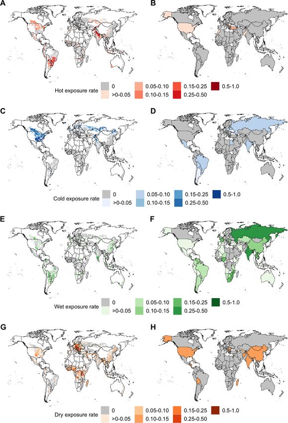
are increasingly exposed. Sugarbeets and potatoes in 3.3. Comparison between ARES and EM-DAT
the Middle East & North Africa and Latin America & We map extremes by weather type calculated with
Caribbean regions are most impacted by extreme wet ARES and EM-DAT for comparison in figure 7.
events. However, rice in North America is estimated Note that ARES is designed to specifically quantify
to be the region and crop most impacted by extreme extremes in agriculture, with a particular emphasis
wet events. Groundnuts, barley, and potatoes in the on crop-specific extremes. Conversely, EM-DAT is a
South Asia region, in addition to soybeans in North well-established database of extreme weather events,
America, have the highest relative change in extreme but it is not specifically developed to capture agri-
dryness. cultural extremes. As such, the two databases capture
14Environ. Res. Lett. 16 (2021) 064006 N D Jackson et al
Figure 7. Comparison between gridded ARES (left column) and country-level EM-DAT (right column) exposure rates by weather
event for the year 2000. Row one is extreme heat, row two is extreme cold, row three and is extreme wetness, and row four is
extreme dryness. Note that ARES reports crop-specific extremes while EM-DAT is not restricted to agricultural hazards.
different events and a comparison between the two is means that biases in reporting will exist in the data,
not a true ‘apples to apples’ comparison. Additionally, including under-representation of countries that do
EM-DAT relies on countries to report extreme events not have the capacity to measure and report such
in order to incorporate them into the database, which events. However, EM-DAT is the most comprehensive
15Environ. Res. Lett. 16 (2021) 064006 N D Jackson et al
database of weather extremes and is widely used by (i.e. through the 2050 s), which we do not do here.
the environmental research community. However, we do build on the work by Gourdji et al
The approach that we have developed here in [10] by including both temperature extremes (e.g.
the ARES model provides increased precision for extreme cold in addition to extreme heat) and mois-
agricultural extremes. Notably, weather extremes in ture extremes (e.g. too wet and too dry) across a
ARES are specifically defined by the physiological longer historical period.
thresholds of crops. Conversely, events in EM-DAT Zhu and Troy [12] assessed agriculturally relev-
are likely those that have the largest financial impact, ant climate extremes during the growing season for
which may or may not occur in agriculture. ARES maize, wheat, soybean, and rice from 1951 to 2006.
applies a consistent definition of extremes through- One metric used by Zhu and Troy [12] is growing
out the entire study domain to climate data that is degree days (GDD), which is the integral of temper-
not biased by weather impact. Reporting procedures ature above a threshold temperature for the staple
have likely changed in time, making it difficult to crops; see table 1 of Zhu and Troy [12]. We extend
compares extremes over time in EM-DAT. Figure 7 this approach by normalizing the number of days
also shows that ARES produces gridded maps of exceeding the crop-specific threshold by the number
extremes (see figures 7(A), (C), (E), and (G)), while of days in the calendar or growing year (see phase
EM-DAT extremes are lumped to the country spa- T4 in section 2.2). The added step enables compar-
tial scale (see figures 7(B), (D), (F), and (H)). This ison across different crops and regions by account-
enables us to pick up on sub-national events, such ing for both crop and spatial variations in growing
as extreme heat in Northern India and drought in seasons. An additional critical difference between this
Eastern Europe and Africa, which is not captured by work and Zhu and Troy [12] is our modification
the EM-DAT data (see figures 7(B), (H)). We provide of SPEI to incorporate crop-specific water demands
cross-sectional comparison between ARES and EM- with crop coefficients (e.g. k; see section 2.3) instead
DAT in figure 7, but note that we compare both data- of the Palmer Drought Severity Index (among other
bases for the entire study domain the SI. Additional metrics) to estimate moisture extremes.
details on how ARES and EM-DAT compare with Our results compare favorably with Zhu and Troy
one another are provided in the SI (see section 3 [12]. Both studies find that there have been more
and tables S11–S13). dry events, particularly since the 1980s, and there is
generally good geographic agreement, such as more
4. Discussion drought in East Asia. Additionally, both studies show
that there has been an increase in exposure to hot tem-
4.1. Comparison with prior studies peratures for wheat and soy. Our results diverge for
This paper builds upon the literature that seeks to extreme heat in maize and rice. This is likely due to
understand the weather conditions crops have histor- the different temperature thresholds used. Zhu and
ically experienced globally. Here, we compare ARES Troy [12] use a threshold of 30◦ C for maize and rice,
output to prior work by Gourdji et al [10] and Zhu while ARES uses 42.0◦ C for maize and 35.4◦ C for rice.
and Troy [12], who also use crop-specific thresholds We associate the lack of warming trend in this study
to define their thermal events. However, this study to the higher maximum temperature thresholds for
distinguishes itself by conducting the analysis at a these crops compared to Zhu and Troy [12].
finer spatial resolution (i.e. 0.25◦ versus 0.5◦ [10]
and 1◦ [19]), for more crops (i.e. 17 versus 4), and 4.2. Limitations in the ARES database and
incorporating annually varying crop-specific land use approach
information versus fixed crop locations. We also look There are several limitations in the methodology of
at both tails of temperature and moisture extremes ARES that limit how it should be used. Farmer adapt-
(e.g. too hot/cold and too wet/dry). ations to climate change and weather extremes are
Gourdji et al [10] assessed the exposure of maize, difficult to quantify and are not captured by our
rice, soybean and wheat to critically high temperat- approach. Importantly, we do not consider how crop
ures during the growing season from 1980 to 2011. physiological thresholds change with time. Genetic
Importantly, Gourdji et al [10] show a weak corres- breeding of crops means that specific crops may
pondence between mean growing season temperat- develop different tolerance levels that we do not cap-
ure and exposure to extreme heat, emphasizing the ture in this study. Additionally, we do not account for
importance of quantifying weather extremes separ- spatial variations in crop thresholds. Different grow-
ately, as we do in this study. Gourdji et al [10] find ing regions may grow different varietals of the same
increasing exposure to extreme heat over the past few crop – with different abilities to withstand weather
decades for wheat in Central and South Asia as well as extremes – that our approach does not consider. The
South America, which compares well with our find- same is true for sowing and planting dates. Temporal
ings (see figure 7(A) and supporting information). and spatial changes in crop growing seasons are not
Gourdji et al [10] additionally project the exposure captured in this study and represent an important
of the staple crops to high temperature in the future future research area.
16Environ. Res. Lett. 16 (2021) 064006 N D Jackson et al
Due to data limitations, we do not estimate expos- 5. Conclusions
ure to extremes for irrigated vs. rainfed crop agricul-
ture. Crops that have access to irrigation will likely The ARES model framework and database was intro-
not have their yields impacted following exposure duced to comprehensively and consistently evaluate
to climate extremes as much as rainfed crops. This crop-specific exposure to extreme weather for the
is because irrigation has been shown to buffer the last half-century. Importantly, we conduct a thorough
impact of climate extremes on crop yields [17, 19, 24]. literature review of agronomic research to incorpor-
Unfortunately, global databases on irrigation water ate crop-specific weather thresholds into our defin-
use by crop are not available, which is what would be ition of extreme events (for both temperature and
needed for our crop-specific study. We do not capture moisture). We integrate these crop-specific attrib-
irrigation expansion over time, another important utes with climate data and crop locations to evaluate
adaptation to climate change and weather extremes. weather extremes in time and space. The framework
This is a shortcoming of our approach and model out- used to develop ARES enables systematic comparis-
put that should caution its use. ons of changes in exposure rates across time, space,
The current framework does not consider com- and crop with and without crop-specific paramet-
pound exposure (e.g. extreme heat and dryness ers. ARES allows us to track which countries, crops,
occurring simultaneously). Future work could and years have had the greatest exposure to extreme
extend the ARES framework to evaluate crop- weather over time. Importantly, we quantify exposure
specific compound events. The crop-specific loca- and not necessarily impact which makes direct com-
tions used within ARES are themselves estimates, parison with existing datasets difficult (e.g. with EM-
and future efforts to collect agricultural locations DAT) and highlights the importance of linking expos-
through government censuses through time would ure with impact (e.g. crop yield and production
enhance reliability. These improvements would losses, economic impacts) in future work.
enable researchers to better determine the drivers This research represents an advancement in terms
of changes in agricultural extremes. of integrating crop characteristics with weather data
to establish models of extremes in agriculture. Critic-
4.3. Future research directions ally, we make the ARES model output available with
Future research could improve on the limitations that this publication, to enable future research to build on
we outlined in section 4.2. For example, information these efforts. Many critical assumptions and limita-
on time-varying crop physiological thresholds could tions accompany this work (detailed in section 4), so
be used to develop more precise estimates of crop the ARES model output should be used with care.
exposure to extremes. The specific varietals used in
different growing regions could be used to spatially Data availability statement
vary the thresholds used by ARES. Understanding
how farmers adapt to weather extremes by adopt- All data sources are detailed in table 1 and are
ing new crop varietals is an important area of future publicly available. We gratefully acknowledge these
research. Relatedly, farmers can adapt to extreme sources, without which this work would not be
weather by choosing to grown certain crops in differ- possible. Output from the Agriculturally-Relevant
ent locations. This is another important area of ongo- Exposure to Shocks (ARES) model is available at
ing research [56] that future applications of ARES the persistent link https://doi.org/10.13012/B2IDB-
could potentially contribute to. Future work could 5457902_V1. The DOI for the dataset associated with
also examine projected climate extremes by crop. this study is 10.13012/B2IDB-5457902_V1
This study quantifies the exposure of specific
crops to extreme weather during the growing season, Acknowledgments
because these events may negatively impact yields.
By definition, our climate thresholds should capture This material is based upon work supported by
negative yield anomalies, since they were collected the National Science Foundation Grant No. EAR-
from the experimental plant biology literature for this 1534544 (‘Hazards SEES: Understanding Cross-
purpose. However, as mentioned in section 4.2 we Scale Interactions of Trade and Food Policy to
do not include irrigation in this study due to data Improve Resilience to Drought Risk’), ACI-1639529
limitations–which may limit the influence of weather (‘INFEWS/T1: Mesoscale Data Fusion to Map and
extremes on crop yield–so future work is needed to Model the U.S. Food, Energy, and Water (FEW)
link the ARES database with yield impact. Rigorously System’), CBET-1844773 (‘CAREER: A National
linking the ARES database with yield data is bey- Strategy for a Resilient Food Supply Chain’), and
ond the scope of the current study, but represents an DEB-1924309 (‘CNH2-L: Feedbacks between Urban
opportunity for future research. To this end, inform- Food Security and Rural Agricultural Systems’). Any
ation on irrigation water use by crop is an important opinions, findings, and conclusions or recommend-
research need for the future. ations expressed in this material are those of the
17You can also read