Influence of the El Niño-Southern Oscillation on entry stratospheric water vapor in coupled chemistry-ocean CCMI and CMIP6 models
←
→
Page content transcription
If your browser does not render page correctly, please read the page content below
Atmos. Chem. Phys., 21, 3725–3740, 2021
https://doi.org/10.5194/acp-21-3725-2021
© Author(s) 2021. This work is distributed under
the Creative Commons Attribution 4.0 License.

Influence of the El Niño–Southern Oscillation on entry stratospheric
water vapor in coupled chemistry–ocean CCMI and CMIP6 models
Chaim I. Garfinkel1 , Ohad Harari1 , Shlomi Ziskin Ziv1,2,3 , Jian Rao1,4 , Olaf Morgenstern5 , Guang Zeng5 ,
Simone Tilmes6 , Douglas Kinnison6 , Fiona M. O’Connor7 , Neal Butchart7 , Makoto Deushi8 , Patrick Jöckel9 ,
Andrea Pozzer10,11 , and Sean Davis12
1 The  Fredy and Nadine Herrmann Institute of Earth Sciences, Hebrew University of Jerusalem, Jerusalem, Israel
2 Department  of Physics, Ariel University, Ariel, Israel
3 Eastern R&D center, Ariel, Israel
4 Key Laboratory of Meteorological Disaster of China Ministry of Education (KLME), Joint International Research

Laboratory of Climate and Environment Change (ILCEC), Collaborative Innovation Center on Forecast and Evaluation
of Meteorological Disasters (CIC-FEMD), Nanjing University of Information Science & Technology,
Nanjing 210044, China
5 National Institute of Water and Atmospheric Research, Wellington, New Zealand
6 National Center for Atmospheric Research, Boulder, Colorado, USA
7 Met Office Hadley Centre, Exeter, UK
8 Meteorological Research Institute, Tsukuba, Japan
9 Deutsches Zentrum für Luft- und Raumfahrt (DLR), Institut für Physik der Atmosphäre, Oberpfaffenhofen, Germany
10 Atmospheric Chemistry Department, Max Planck Institute for Chemistry, 55128 Mainz, Germany
11 International Centre for Theoretical Physics, Trieste, Italy
12 NOAA Chemical Sciences Laboratory, Boulder, CO, USA

Correspondence: Chaim I. Garfinkel (chaim.garfinkel@mail.huji.ac.il)

Received: 30 July 2020 – Discussion started: 10 September 2020
Revised: 19 January 2021 – Accepted: 25 January 2021 – Published: 11 March 2021

Abstract. The connection between the dominant mode of            models find that this moistening persists, and some show a
interannual variability in the tropical troposphere, the El      nonlinear response, with both El Niño and La Niña leading to
Niño–Southern Oscillation (ENSO), and the entry of strato-       enhanced water vapor in both winter, spring, and summer. A
spheric water vapor is analyzed in a set of model simulations    moistening in the spring following El Niño events, the signal
archived for the Chemistry-Climate Model Initiative (CCMI)       focused on in much previous work, is simulated by only half
project and for Phase 6 of the Coupled Model Intercompar-        of the models. Focusing on Central Pacific ENSO vs. East
ison Project. While the models agree on the temperature re-      Pacific ENSO, or temperatures in the mid-troposphere com-
sponse to ENSO in the tropical troposphere and lower strato-     pared with temperatures near the surface, does not narrow the
sphere, and all models and observations also agree on the        inter-model discrepancies. Despite this diversity in response,
zonal structure of the temperature response in the tropical      the temperature response near the cold point can explain the
tropopause layer, the only aspect of the entry water vapor re-   response of water vapor when each model is considered sep-
sponse with consensus in both models and observations is         arately. While the observational record is too short to fully
that La Niña leads to moistening in winter relative to neu-      constrain the response to ENSO, it is clear that most models
tral ENSO. For El Niño and for other seasons, there are sig-     suffer from biases in the magnitude of the interannual vari-
nificant differences among the models. For example, some         ability of entry water vapor. This bias could be due to biased
models find that the enhanced water vapor for La Niña in         cold-point temperatures in some models, but others appear
the winter of the event reverses in spring and summer, some

Published by Copernicus Publications on behalf of the European Geosciences Union.
3726                               C. I. Garfinkel et al.: ENSO and entry stratospheric water vapor in CCMI and CMIP6

to be missing forcing processes that contribute to observed        few decades, also shows a clear moistening after the 1982–
variability near the cold point.                                   1983 event (Fig. 3 of Wang et al., 2020). Strong La Niña
                                                                   (LN) events in 1998–1999 and 1999–2000 also clearly pre-
                                                                   ceded elevated water vapor concentrations in the tropical
                                                                   lower stratosphere. The net effect of more moderate events
1   Introduction                                                   (either LN or EN) is unclear (Gettelman et al., 2001), and
                                                                   there may be a nonlinear effect. Specifically, Garfinkel et al.
Water vapor is the gas with most important greenhouse effect       (2018) found that both strong EN and LN events lead to
in the atmosphere, and the feedback associated with strato-        elevated water vapor concentrations compared with neutral
spheric water vapor in response to increasing anthropogenic        ENSO in a chemistry–climate model, and indeed such an ef-
greenhouse gas emissions is around half of that for global         fect is weakly evident (although not significant) in observa-
mean surface albedo or cloud feedbacks (Forster and Shine,         tions (Fig. 4 of Garfinkel et al., 2018). In addition, there is
1999; Solomon et al., 2010; Dessler et al., 2013; Banerjee         a strong seasonal dependence of the effect of EN on strato-
et al., 2019; Li and Newman, 2020). The amount of water            spheric water vapor, with the increase in water vapor for EN
vapor entering the stratosphere also regulates the severity        and decrease for LN occurring mainly in boreal spring (Calvo
of ozone depletion (Solomon et al., 1986) and is important         et al., 2010; Garfinkel et al., 2013; Konopka et al., 2016; Tao
for other aspects of stratospheric chemistry (Dvortsov and         et al., 2019).
Solomon, 2001). Hence, it is important to understand how              The limited duration of the observational data record,
the comprehensive models that are used for projections of          and the importance of other atmospheric processes (e.g.,
future ozone and climate capture the processes regulating the      the quasi-biennial oscillation), which may interact nonlin-
entry of stratospheric water vapor.                                early with ENSO (Yuan et al., 2014), limit the confidence
   Lower-stratospheric water vapor concentrations are              with which observed variability during and following ENSO
mainly determined by the tropical temperatures near the            events can be unambiguously associated with ENSO. Sev-
cold point, where dehydration takes place as air parcels           eral studies have used simulations from single models to try
transit into the stratosphere (Mote et al., 1996; Zhou et al.,     to understand the role of ENSO with respect to entry strato-
2004, 2001; Fueglistaler and Haynes, 2005b; Fueglistaler           spheric water vapor (Scaife et al., 2003; Garfinkel et al.,
et al., 2009; Randel and Park, 2019). Several different            2013; Brinkop et al., 2016; Garfinkel et al., 2018; Ding and
processes have been shown to influence these cold-point            Fu, 2018), although it is not clear whether the results are
temperatures, and the goal of this work is to revisit the          general to other models. The goal of this study is to con-
influence of one of these processes – the El Niño–Southern         sider a wider range of models, with a combined model out-
Oscillation (ENSO) – on entry water vapor in the lower             put of over 2700 years, in order to better understand the re-
stratosphere.                                                      sponse of stratospheric water vapor to ENSO. We focus here
   El Niño (EN), the ENSO phase with anomalously warm              on chemistry–climate models, as these models must reason-
sea surface temperatures in the tropical East Pacific, leads       ably simulate entry water vapor, otherwise their stratospheric
to a warmer tropical troposphere and cooler tropical lower         chemistry will suffer from biases.
stratosphere (Free and Seidel, 2009; Calvo et al., 2010; Simp-        After introducing the data and methodology in Sect. 2, we
son et al., 2011), with the zero-crossing in the vicinity of the   contrast the impact of ENSO on stratospheric water vapor
cold point (Hardiman et al., 2007). In addition, EN leads to       in 12 different chemistry–climate models. Even though all
a zonal dipole in temperature anomalies near the tropopause        models simulate a similar response to ENSO in the tropo-
and, in particular, to a Rossby wave response with anoma-          sphere and also in the lower stratosphere (warming and cool-
lously warm temperatures over the Indo-Pacific warm pool           ing, respectively), there is no consensus as to the impact of
and anomalously cold temperatures over the Central Pacific         ENSO on stratospheric water vapor. Some models simulate
(Yulaeva and Wallace, 1994; Randel et al., 2000; Zhou et al.,      enhanced water vapor for EN in both the winter of the event
2001; Scherllin-Pirscher et al., 2012; Domeisen et al., 2019).     and the following spring, some models find an opposite re-
In the tropical tropopause layer (TTL), water vapor increases      sponse, and some simulate a nonlinear response, with both
in the region with warm anomalies and decreases in the re-         EN and LN leading to enhanced water vapor in spring (as is
gion with cold anomalies by ∼ 25 % (Gettelman et al., 2001;        evident in GEOSCCM, Garfinkel et al., 2018). In all cases,
Hatsushika and Yamazaki, 2003; Konopka et al., 2016).              the temperature response near the cold point can explain the
   The net effect of these zonally asymmetric and symmetric        divergent responses of water vapor to ENSO.
changes on water vapor above the tropical cold point is com-
plex. The two largest EN events in the satellite era (in 1997–
1998 and in 2015–2016) were followed by moistening of the
tropical lower stratosphere (Fueglistaler and Haynes, 2005a;
Avery et al., 2017; Diallo et al., 2018), and the ERA5 re-
analysis, which tracks satellite water vapor well over the last

Atmos. Chem. Phys., 21, 3725–3740, 2021                                             https://doi.org/10.5194/acp-21-3725-2021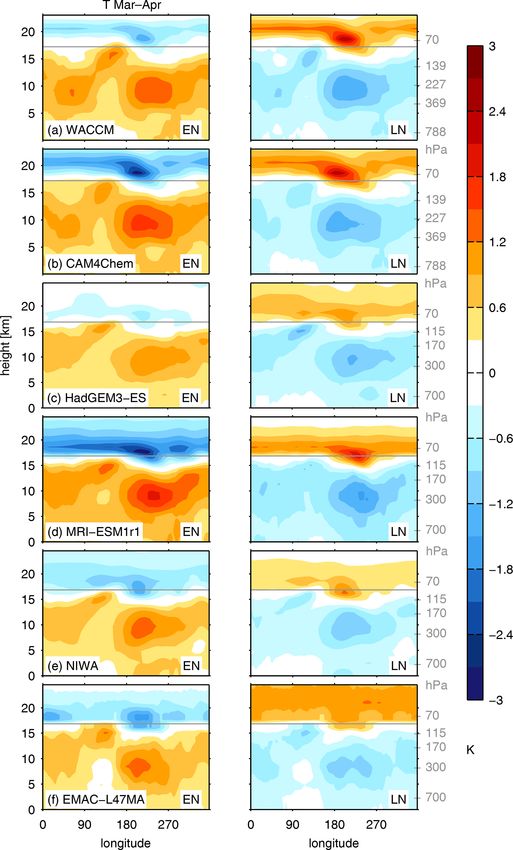
C. I. Garfinkel et al.: ENSO and entry stratospheric water vapor in CCMI and CMIP6                                                  3727

2     Data and methods

2.1    Data

We examine six models participating in the Chemistry-
Climate Model Initiative (CCMI; Morgenstern et al., 2017)
and six models participating in Phase 6 of the Coupled Model
Intercomparison Project (CMIP6; Eyring et al., 2016). How-
ever, the focus in most of this paper is on the CCMI models,
for which data are archived at a higher vertical resolution,
as this allows for a more careful diagnosis of the physical
processes. Coupled chemistry–climate models are expected
to have more robust interannual variability in temperatures
in the lower stratosphere compared with models with fixed
ozone (Yook et al., 2020); hence, we only include CMIP6
models with interactive stratospheric chemistry.
   CCMI was jointly launched by the Stratosphere-
troposphere Processes And their Role in Climate (SPARC)
and the International Global Atmospheric Chemistry (IGAC)
projects to better understand chemistry–climate interactions
in the recent past and future climate (Eyring et al., 2013;
Morgenstern et al., 2017). This modeling effort is an ex-
tension of CCMVal2 (SPARC-CCMVal, 2010), but it uti-
lizes up-to-date chemistry–climate models that also include
tropospheric chemistry. We consider the Ref-C2 simula-
tions, which span the 1960–2100 period, impose ozone-
depleting substances reported by the World Meteorologi-
cal Organization (2011), and impose greenhouse gases other        Figure 1. Anomalous 80 hPa water vapor in WACCM compared
than ozone-depleting substances as in Representative Con-         with the value of the Nino3.4 index for (a) November and Decem-
centration Pathway (RCP) 6.0 (Meinshausen et al., 2011).          ber, (b) January and February, (c) March and April, and (d) May and
The full details of these simulations are described by Eyring     June. Each dot corresponds to 1 model year. When a polynomial fit
et al. (2013). Note that the GEOSCCM simulations provided         better describes the dependence on ENSO than a linear fit, we show
to CCMI did not have a coupled ocean, but Garfinkel et al.        the R 2 for a linear fit and the adjusted R 2 for the polynomial fit (see
(2018) have already examined the ENSO–water vapor con-            Sect. 2.2). Otherwise we show a linear least squares best fit in each
nection in this model in a coupled ocean configuration. As        panel.
we are interested in connections between ENSO and the
stratosphere, we only consider CCMI models with a coupled
                                                                  contrast, CCMI output is available both near 80 and 90hPa.)
ocean in which ENSO develops spontaneously. We consider
                                                                  All of the CCMI models and all of the CMIP6 models except
all available ensemble members. The CCMI models used in
                                                                  GISS-E2-1-G represent the quasi-biennial oscillation (QBO)
this study are listed in Table 1. Harari et al. (2019) showed
                                                                  (Rao et al., 2020a; Richter et al., 2020; Rao et al., 2020b). In
that each of these models simulates surface temperature vari-
                                                                  total, more than 2700 years of model output are available.
ability in the Nino3.4 region similar to that observed.
                                                                     Model output is compared to model-level temperatures
   In addition to the CCMI models, we also consider six
                                                                  in the ERA5.1 reanalysis (Hersbach et al., 2020) and wa-
Earth system models with coupled chemistry that are par-
                                                                  ter vapor from 1993 through 2019 in version 2.6 of the
ticipating in CMIP6: CESM2-WACCM (Gettelman et al.,
                                                                  SWOOSH dataset (specifically the combinedeqfillanomfill
2019), GFDL-ESM4 (Dunne et al., 2019), CNRM-ESM2-1
                                                                  product, Davis et al., 2016). ERA5 assimilates available
(Séférian et al., 2019), GISS-E2-1-G (Kelley et al., 2019),
                                                                  satellite and GPS data in the tropical tropopause layer and has
MRI-ESM2-0 (Yukimoto et al., 2019), and UKESM1-0-LL
                                                                  a higher vertical resolution (approximately 300 m in the trop-
(Sellar et al., 2019). The seasonal cycle and climatology of
                                                                  ical tropopause layer) than any previous reanalyses (Hers-
stratospheric water vapor for five of these models is docu-
                                                                  bach et al., 2020).
mented in Keeble et al. (2020). For these models, we fo-
cus on the historical integrations of the period from 1850
to 2014. Note that standard CMIP6 output includes the 70
and 100 hPa levels but no level in between, which limits our
ability to diagnose physical processes near the cold point. (In

https://doi.org/10.5194/acp-21-3725-2021                                             Atmos. Chem. Phys., 21, 3725–3740, 2021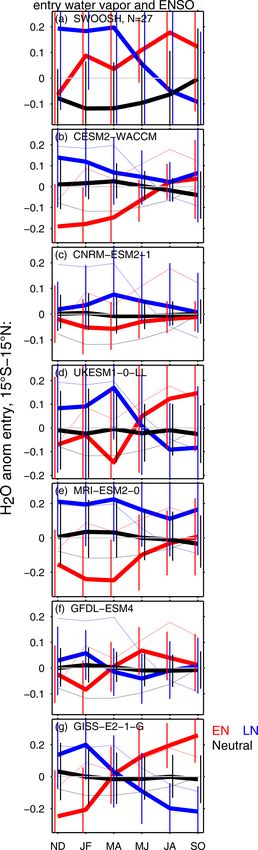
3728                                   C. I. Garfinkel et al.: ENSO and entry stratospheric water vapor in CCMI and CMIP6

Table 1. The data sources used in this study. For CMIP6 models, we focus on the historical integrations of the period from 1850 to 2014; for
CCMI, we focused on the Ref-C2 simulations spanning the period from 1960 to 2100.

                                                 Data source             Ensemble    Reference
                                                                         members
                               Observations      SWOOSH v2.6                1        Davis et al. (2016)
                                                 ERA5                       1        Hersbach et al. (2020)
                               CCMI              NIWA-UKCA                  5        Morgenstern et al. (2009)
                                                 CESM1 WACCM                3        Garcia et al. (2017)
                                                 CESM1 CAM4-chem            3        Tilmes et al. (2016)
                                                 HadGEM3-ES                 1        Hardiman et al. (2017)
                                                 MRI-ESM1r1                 1        Yukimoto et al. (2012)
                                                 EMAC-L47MA                 1        Jöckel et al. (2016)
                               CMIP6             CESM2-WACCM                1        Gettelman et al. (2019)
                                                 GFDL-ESM4                  1        Dunne et al. (2019)
                                                 CNRM-ESM2-1                1        Séférian et al. (2019)
                                                 GISS-E2-1-G                1        Kelley et al. (2019)
                                                 MRI-ESM2-0                 1        Yukimoto et al. (2019)
                                                 UKESM1-0-LL                1        Sellar et al. (2019)

Table 2. Note that the pressure level for each model differs due to       lag to track the QBO. We compute the QBO separately for
data availability, and the levels used for this chart are indicated in    each data source. Tao et al. (2019) found a maximum cor-
Fig. 2.                                                                   relation for a 1-month lag, whereas we find the correlation
                                                                          is higher for a longer lag (not shown), although our con-
          Correlation coefficient (R) between entry water                 clusions are unchanged if we use 1 month. For consistency,
                 vapor and cold-point temperature                         this same MLR procedure is applied to CCMI, CMIP6, and
                            Zonal averaged T ,     The 20 %               ERA5/SWOOSH data.
                                 15◦ S–15◦ N        quintile                 Each CCMI model makes data available at different pres-
                                                                          sure or sigma levels, which limits the precision with which
        WACCM                            −0.28          0.73
        CAM4Chem                         −0.26          0.41
                                                                          we can compare models. However, differences in the pres-
        HadGEM3-ES                        0.42          0.75              sure levels at which data are available are generally less than
        MRI-ESM1r1                        0.50          0.58              2 hPa, and we consider anomalies of each model from its own
        NIWA-UKCA                         0.54          0.96              climatology. When considering entry water vapor for CCMI,
        EMAC-L47MA                        0.35          0.69              we examine the level closest to 80 hPa, and when consider-
                                                                          ing the cold-point temperature, we examine the level closest
                                                                          to 90 hPa archived by each CCMI model. The specific levels
                                                                          chosen for each CCMI model are indicated in the figures.
2.2    Methods                                                               For ENSO, we use surface air temperature in the region
                                                                          bounded by 5◦ S–5◦ N and 190◦ E–240◦ E (i.e., the Nino3.4
This study focuses on the impact of ENSO on the strato-                   region), as sea surface temperature was not available for all
sphere on interannual timescales; in order to remove any im-              models at the time we downloaded the data. A composite
pacts on longer timescales due to climate change and also                 of EN events is formed if the average temperature in the
to remove any linear impacts from the quasi-biennial oscilla-             Nino3.4 region in November through February (NDJF) rel-
tion, which is known to affect water vapor (Reid and Gage,                ative to each model’s climatology exceeds 1 K, whereas a
1985; Zhou et al., 2001, 2004; Fujiwara et al., 2010; Liang               composite of LN events is formed if the average temperature
et al., 2011; Kawatani et al., 2014; Brinkop et al., 2016),               anomaly is less than −1 K. All other years are categorized as
we first use multiple linear regression (MLR) to remove the               neutral ENSO. A typical ENSO event slowly strengthens in
linear variability associated with greenhouse gases and the               the summer and fall, reaches its maximum strength in late fall
QBO from all time series (i.e., the same regression is applied            or early winter, and then decays in the spring (Fig. 1 of Wang
to temperature and water vapor). We use historical CO2 con-               and Fiedler, 2006). This evolution is captured in the models
centrations for historical simulations and the equivalent CO2             (Fig. S1 in the Supplement). While the influence of ENSO on
from the RCP6.0 scenario to track future greenhouse gas con-              tropospheric temperatures is rapid due to convection, there is
centrations (Meinshausen et al., 2011) as well as zonal aver-             a lag of a few months in the transport from the level with
aged zonal winds from 5◦ S to 5◦ N at 50 hPa with a 2-month

Atmos. Chem. Phys., 21, 3725–3740, 2021                                                    https://doi.org/10.5194/acp-21-3725-2021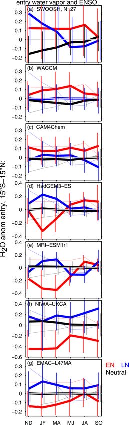
C. I. Garfinkel et al.: ENSO and entry stratospheric water vapor in CCMI and CMIP6 3729
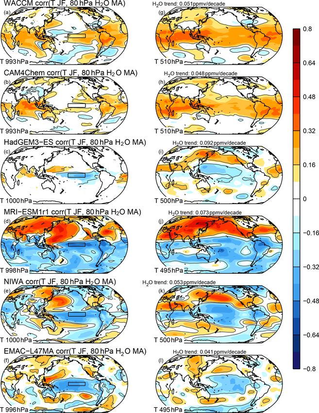
Figure 2. Tropical water vapor from 15◦ S to 15◦ N near 80 hPa in each of the six CCMI models considered here from the late fall as
the event is developing through to the following summer for (red) El Niño, (blue) La Niña and (black) neutral ENSO (left column). The
5 % confidence intervals on the anomalous response based on a two-tailed Student’s t test are shown. The response of zonally averaged
temperature anomalies from 15◦ S to 15◦ N near 90 hPa for each model (middle column). The evolution of the temperature of the coldest
20 % of the tropics at 90 hPa for each model in each ENSO phase compared with the model’s climatology (right column).
peak convective outflow to the cold point (Mote et al., 1996; preferred if the adjusted R 2 for the polynomial fit is larger by
Fueglistaler et al., 2004). However, the sea surface tempera- any amount compared with the linear R 2 , although we only
ture anomalies due to ENSO are already established by fall; show the polynomial fit if the adjusted R 2 exceeds the R 2
hence, all of the anomalies shown here are associated with for a linear fit by 33 %. Note that the 33 % criterion is sub-
ENSO. jectively chosen, although results are similar for a slightly
Statistical significance of the composite mean response to modified criterion.
a given ENSO phase is determined using a Student’s t test.
The adjusted R 2 (Eq. 3.30 of Chatterjee and Hadi, 2012) is
used to quantify the added value in using a polynomial best 3 Results
fit (e.g., H2 O ∼ a · EN2 + b · EN) instead of a linear best fit
(e.g., H2 O ∼ c · EN). The adjusted R 2 considers the likeli- We begin with the water vapor response to ENSO in the
hood that a polynomial predictor will reduce the residuals by WACCM simulation included in CCMI in Fig. 1. At 90 hPa
unphysically over-fitting the data. The polynomial fit can be and also at higher pressure levels (i.e., lower in the TTL), EN
https://doi.org/10.5194/acp-21-3725-2021 Atmos. Chem. Phys., 21, 3725–3740, 2021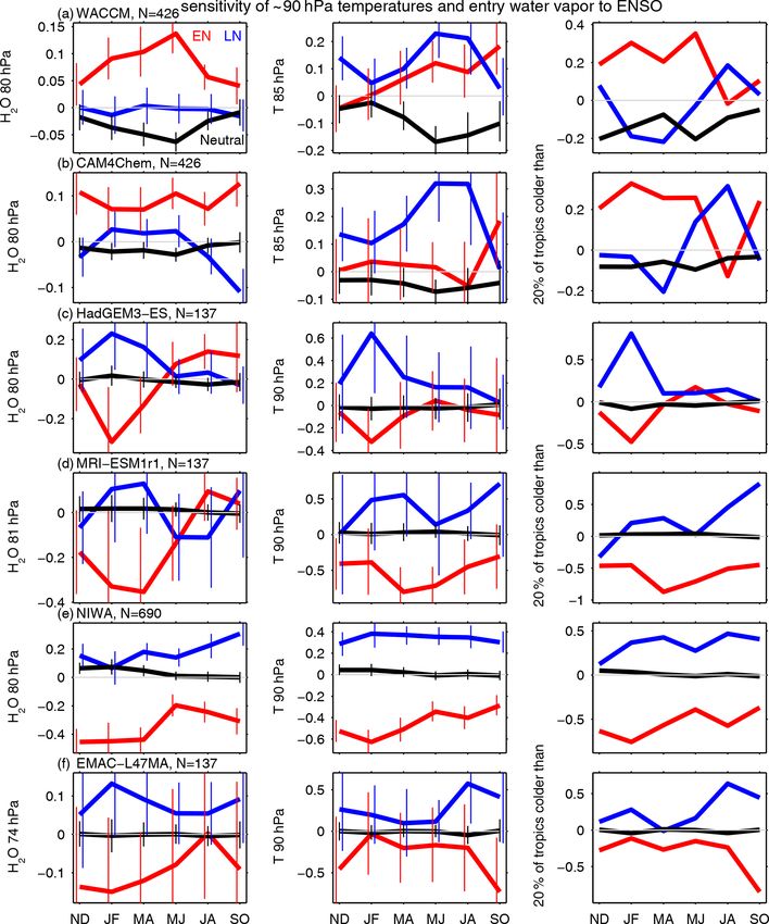
3730                                C. I. Garfinkel et al.: ENSO and entry stratospheric water vapor in CCMI and CMIP6

leads to enhanced water vapor and LN leads to reduced water
vapor in both winter and spring. Convection can rapidly mix
moist boundary layer air with the TTL (e.g., Levine et al.,
2007). Above the cold point, however, the water vapor re-
sponse is not significant in November and December, but it
then shows a distinct nonlinearity in subsequent months, with
both EN and LN leading to enhanced water vapor. This non-
linear effect is similar to that seen in the GEOSCCM model
by Garfinkel et al. (2018) and is also similar to the effect in
SWOOSH observational data (Fig. 1).
   These results are summarized in Fig. 2a, which shows the
water vapor response for EN (the events in the right shaded
box in Fig. 1), LN (the events in the left shaded box in Fig. 1),
and neutral ENSO (all other events). In January through June,
both EN and LN lead to significantly more entry water vapor
than neutral ENSO. The pronounced moistening during EN
peaks in the spring after the event has already begun to decay.
These effects are all consistent with that seen in GEOSCCM
in Garfinkel et al. (2018). A generally similar effect is evident
in CAM4Chem, which shares code with WACCM.
   The four models shown in Fig. 2c, d, e, and f have a qual-
itatively different response to ENSO than the NCAR models
and GEOSCCM. Specifically, HadGEM3-ES, NIWA, MRI-
ESM1r1, and EMAC-L47MA all simulate somewhat more
water vapor for LN than neutral ENSO (although this effect
is generally not statistically significant), and significantly
more water vapor for neutral ENSO than EN, in January
through April. In NIWA and EMAC-L47MA this effect ex-
tends through all calendar months.
   This large diversity in the entry water vapor response
to ENSO occurs despite the fact that all models simulate
a qualitatively similar response in tropospheric and lower-
stratospheric temperatures, as we now demonstrate.
   Figure 3 shows the distribution of 15◦ S–15◦ N tempera-
ture as a function of longitude and height for these six mod-       Figure 3. Longitude vs. height cross section of the 15◦ S–15◦ N
els in March and April, the months with the strongest dis-          temperature anomalies during (left) El Niño and (right) La Niña in
parity among the models in the response of entry water to           each of the CCMI models. The Supplement presents map views of
ENSO, and a map view of the temperature anomalies at 100            temperature anomalies at 70 and 100 hPa.
and 70 hPa are included in the Supplement.
   All models are characterized by a more pronounced tro-
pospheric warming between 200◦ E and 250◦ E immediately             in the tropics near 90 hPa. The zonally averaged tempera-
above the region with warming sea surface temperatures              ture response to ENSO in WACCM has little resemblance to
compared with other longitudes, and there is a zonal mean           the water vapor response. Rather, the water vapor response
increase in temperature throughout the troposphere in all           can be better understood by focusing on the coldest region of
models. The tropospheric warming peaks in the upper tro-            the tropics. Due to the relative slowness of vertical transport
posphere and extends up to the TTL near 120◦ E in all mod-          compared with horizontal transport in the tropical tropopause
els. Furthermore, all models simulate a lower-stratospheric         layer, entry water vapor is sensitive to the coldest regions
cooling (above 70 hPa) in response to EN and a warming in           in the tropics and not just zonal mean temperatures (i.e.,
response to LN. While the magnitude of these features differs       the cold point; Mote et al., 1996; Hatsushika and Yamazaki,
among the model, the patterns are robust.                           2003; Bonazzola and Haynes, 2004; Fueglistaler et al., 2004;
   Near the tropopause, however, there is less agreement            Fueglistaler and Haynes, 2005a; Oman et al., 2008; Randel
among the models in the large-scale temperature response,           and Park, 2019). We quantify this effect as follows: we first
and this difference can account for the large diversity in the      sort the temperature in all grid points from 15◦ S to 15◦ N
water vapor responses to ENSO. The middle column of Fig. 2          in each bimonthly period; we then calculate the threshold
shows the zonally averaged temperature response to ENSO             temperature associated with the first quintile, second quin-

Atmos. Chem. Phys., 21, 3725–3740, 2021                                               https://doi.org/10.5194/acp-21-3725-2021
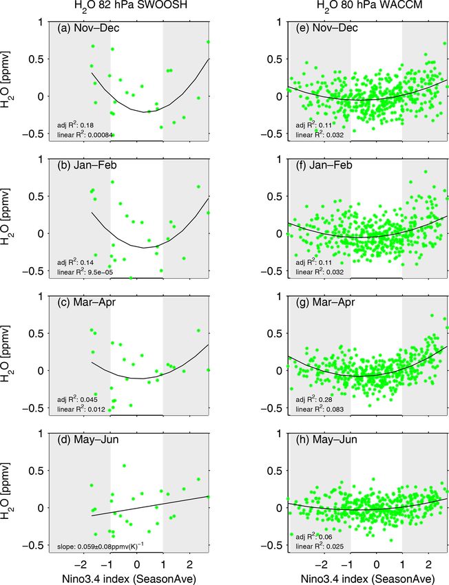
C. I. Garfinkel et al.: ENSO and entry stratospheric water vapor in CCMI and CMIP6                                                 3731

Figure 4. Correlation of (left) near-surface temperature and (right) temperature near 500 hPa with entry water vapor in each of the CCMI
models, with temperature taken for January and February and water vapor for March and April. A black line indicates correlations signifi-
cantly different from zero at the 95 % confidence level.

tile, etc., of tropical temperatures; we compute these quintiles       correlation between the 20 % quintile cold-point temperature
separately for the EN, LN, and neutral ENSO composites                 anomalies and the water vapor anomalies is 0.73 (Table 2).
and then compute the difference for each composite from the            Results are generally similar for CAM4Chem through June:
model climatology. The results of this analysis for the second         the correlation of entry water with the coldest 20 % is pos-
quintile are shown in the right column of Fig. 2a. The coldest         itive, whereas the correlation with zonal mean temperatures
20 % of the tropics is ∼ 0.25 K warmer during EN compared              is not.
with the model climatology from November through June,                    HadGEM3-ES, NIWA, MRI-ESM1r1, and EMAC-
whereas the coldest 20 % of the tropics is colder than the             L47MA all simulate similar temperature responses if we
model climatology for LN and neutral ENSO. Overall, the                focus on the zonal mean or the coldest 20 % of the tropics,

https://doi.org/10.5194/acp-21-3725-2021                                                 Atmos. Chem. Phys., 21, 3725–3740, 2021
3732                                C. I. Garfinkel et al.: ENSO and entry stratospheric water vapor in CCMI and CMIP6

although correlations with entry water vapor are higher if
we focus on the coldest 20 % of the tropics rather than zonal
mean temperature (Table 2). For these models, temperatures
are warmer for LN than neutral ENSO and colder for EN
than neutral ENSO (Table 2). Overall, the temperature
response to ENSO in the coldest 20 % of the tropics near
90 hPa can help account for the substantial inter-model
diversity in the response of entry water to the stratosphere.
    Garfinkel et al. (2013) and Ding and Fu (2018) consid-
ered the possibility that sea surface temperatures (SSTs) in
the Central Pacific may have a different effect on entry water
than SSTs in the East Pacific, and the two studies, using dif-
ferent individual models, found that warmer SSTs in the Cen-
tral Pacific lead to dehydration. We evaluate this effect for the
CCMI models in Fig. 4. Specifically, the left column of Fig. 4
shows the correlation between entry water in March and
April and near-surface temperature in January and February.
There is clearly a wide range of responses evident, and con-
sistent with Fig. 2, some models show a positive correlation
between SSTs in the Nino3.4 region (e.g., WACCM) whereas
others show a negative correlation (HadGEM3-ES, NIWA,
MRI-ESM1r1, and EMAC-L47MA). There is no clear dif-
ference in the correlation between near-surface temperature
to the east or west of the Nino3.4 region (indicated with a
black box in Fig. 4), and there is clearly no consensus among
the models as to whether warmer SSTs in the Central Pacific
lead to dehydration.
    Dessler et al. (2013) and Dessler et al. (2014) find that
tropical tropospheric temperatures at 500 hPa are a better pre-
dictor of entry water vapor than ENSO in the satellite record.
Therefore, we consider the correlation between entry water
in March and April and 500 hPa temperature in January and
February for each model in Fig. 4 (right column). There is
clearly a wide range of responses evident, and the response
is similar in pattern to that in Fig. 4a–f. Specifically, some
models show a positive correlation of entry water with mid-
tropospheric temperatures (e.g., WACCM and CAM4Chem)
whereas others show a negative correlation (HadGEM3-ES,
NIWA, MRI-ESM1r1, and EMAC-L47MA). Note that all
models simulate a long-term moistening trend of the lower
stratosphere if the trend is computed before applying the
MLR described in Sect. 2 (trend indicated above Fig. 4g, h,
i, j, k, and l), and of the six models considered, the two with
the strongest long-term moistening trend simulate a negative
correlation between temperatures at 500 hPa and entry wa-
ter vapor when focusing on interannual variability. Hence,          Figure 5. (a) As in Fig. 2a but for SWOOSH at 82 hPa. (b–g) As in
                                                                    Fig. 2 but subsampling the model output for each model to match
there is no evidence that temperatures at 500 hPa are a more
                                                                    the sample size in observations for each ENSO phase. The uncer-
discriminatory predictor of entry water vapor on interannual
                                                                    tainty (marked with vertical lines) of the model response is deter-
timescales than ENSO. Results are similar if we allow for           mined by Monte Carlo subsampling, as described in the text. The
a 4-month lag between tropospheric temperature and entry            response in Fig. 2a is repeated with a thin line in subsequent panels.
water vapor for five of the six models (Fig. S4). That being
said, it is conceivable that on longer timescales, the magni-
tude of mid-tropospheric warming would be, for example, re-
lated to an upward expansion of the TTL (a robust response
to climate change), and such an expansion of the TTL might

Atmos. Chem. Phys., 21, 3725–3740, 2021                                                https://doi.org/10.5194/acp-21-3725-2021
C. I. Garfinkel et al.: ENSO and entry stratospheric water vapor in CCMI and CMIP6 3733
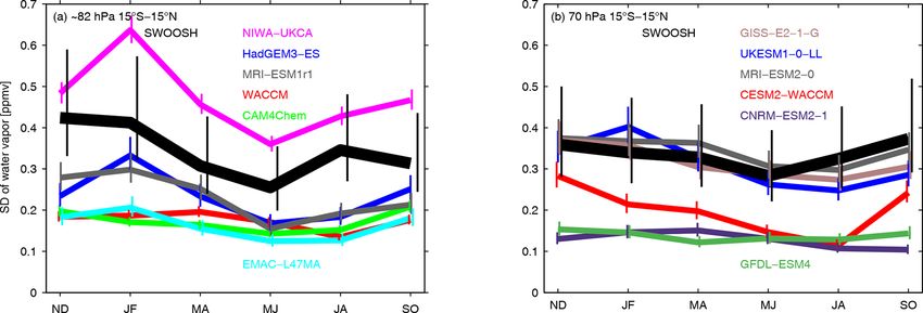
Figure 6. Standard deviation of tropical entry water vapor for each model in (a) CCMI near 82 hPa and (b) CMIP6 at 70 hPa as well as for
SWOOSH water vapor (thick line). The vertical lines denote the 95 % confidence bounds, as discussed in the text.
be expected to lead to more entry water vapor. A thorough tiles of the subsampled response to EN, to which we can
investigation of this possibility is beyond the scope of this compare the observed response.
paper. Figure 5b–g show the response to ENSO in these subsam-
ples for each model, and we repeat the observed response
with a thin line. If the observed response falls outside of the
4 Comparison to observations and CMIP6 middle 95 % of the subsampled response (indicated with a
vertical line), the model response to ENSO is inconsistent
What is the observed response of entry water vapor to with that observed. There is a lack of overlap of the sub-
ENSO? Figure 5a is the same as Fig. 2a but for SWOOSH samples of the model with the observed response for at least
entry water vapor, and while both LN and EN are associated one season or phase for all modeling centers. For some of
with more water vapor, the difference between EN and neu- the CCMI models, the degree of inconsistency is relatively
tral ENSO and between LN and neutral ENSO is not statis- small. Specifically, the response in HadGEM3-ES, WACCM,
tically significant. (Note that if ERA5.1 water vapor is used and CAM4Chem is consistent with observations in most sea-
and the years 1979 to 2019 are considered, the moistening sons and for most phases, with gaps between the vertical bars
for EN is significant in July and August.) Similarly, the re- and the observed response generally being small (Fig. 5b, c,
gression coefficient of a linear best fit of entry water vapor d). The other models, however, suffer from large discrepan-
with ENSO (Fig. 1) is also not statistically significant (and cies between the observed and modeled responses to ENSO
for ERA5.1 water vapor, the increase is significant in July even when we compare similar sample sizes.
and August; details are not shown). Despite the lack of a sig- An additional metric to evaluate differences in observed
nificant effect in observations, the models that appear to be vs. modeled ENSO teleconnections is for the model to sim-
closest to the observed response are the NCAR models and ulate a similar amount of variance compared with that ob-
also the GEOSCCM simulations evaluated by Garfinkel et al. served, as otherwise the model does not satisfactorily capture
(2018). internal atmospheric variability (Deser et al., 2017; Garfinkel
A complication when comparing the models to SWOOSH et al., 2019; Weinberger et al., 2019). Therefore, we compare
entry water is that ∼ 140 years at least of model data are the standard deviation of entry water vapor for each model in
available for each model, whereas only 27 years of data are Fig. 6a. The 95 % confidence interval of the standard devi-
available for observations. Hence, it is ambiguous whether ation as given by a chi-square test is indicated with a ver-
the difference between models and observations reflects an tical line. In boreal winter, only HadGEM3-ES and MRI-
actual model bias or, alternately, might reflect uncertainty ESM1r1 simulate realistic variability, with NIWA simulating
given the small observational sample (i.e., the large error bars too much and the other models simulating too little. In boreal
in Fig. 5a overlap the error bars in Fig. 2 for many models). summer, all models suffer from unrealistic variability.
In order to better compare model and observations, we adopt Recently, at least six coupled ocean–chemistry–climate
a Monte Carlo subsampling technique. Taking EN as an ex- models have participated in CMIP6, and we now assess
ample, we randomly select six EN events from each model the ENSO–water vapor connection in the following mod-
to match the number of observed EN events in the SWOOSH els: CESM2-WACCM, GFDL-ESM4, GISS-E2-1-G, MRI-
period, and we compute the mean entry water vapor anomaly ESM2-0, UKESM1-0-LL, and CNRM-ESM2-1. Of these six
for these events. We then repeat this random sampling 2000 models, three are newer versions or successors of models that
times with different EN events randomly included in the sub- participated in CCMI (CESM2-WACCM, MRI-ESM2-0, and
sample. Finally, we compute the top and bottom 2.5 % quan-
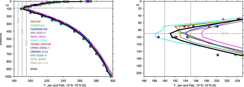
https://doi.org/10.5194/acp-21-3725-2021 Atmos. Chem. Phys., 21, 3725–3740, 20213734 C. I. Garfinkel et al.: ENSO and entry stratospheric water vapor in CCMI and CMIP6 UKESM1-0-LL). Figure 7 is the same as Fig. 5 but for 70 hPa water vapor, as water vapor near 80 hPa is not a standard CMIP6 output variable. The observed water vapor response at 70hPa resembles that at 82 hPa (Fig. 7a vs. Fig. 5a). While the models generally agree that LN leads to moistening in winter, the models simulate a wide diversity of responses in the spring and summer following LN and EN. The modeled response is only consistent with observations for one model, in that the subsampled response from the model encompasses observations (UKESM1-0-LL). For all other models, the ob- served and modeled responses to water vapor are inconsistent in at least one season and one ENSO phase, and while the inconsistency is relatively small for GISS-E2-1-G and MRI- ESM2-0 and to a lesser degree CESM2-WACCM, it is pro- nounced for CNRM-ESM2-1 and GFDL-ESM4. The standard deviation of 70 hPa tropical water vapor for each CMIP6 model is shown in Fig. 6b. While nearly all CCMI models struggled to capture realistic variability, half of the CMIP6 models simulate a realistic amount of variabil- ity. Specifically, the CCMI models HadGEM3-ES and MRI- ESM1r1 failed to simulate realistic variability in spring, but the corresponding CMIP6 models UKESM1-0-LL and MRI- ESM2-0 are realistic. GISS-E2-1-G also simulates a realis- tic amount of variability. However, the other three CMIP6 models simulate too little variability, although the bias in WACCM is smaller in the CMIP6 CESM2-WACCM than in the CCMI version of WACCM in winter. Biases in the standard deviation of entry water have been shown to be associated with biases in cold-point temperature (Hardiman et al., 2015; Brinkop et al., 2016), and such an ex- planation can account for the biased variability in some of the models. Figure 8 shows the climatological zonal mean tem- perature from 10◦ S to 10◦ N in each model in January and February compared with ERA5.1. The NIWA model suffers from an overly warm cold point and, consistent with this, overly strong variability in entry water. EMAC-L47MA and CNRM-ESM2-1 suffer from the opposite problem: an overly cold cold point and too little variability in entry water. The Met Office model used in CMIP5 is known to have a warm cold-point bias (Hardiman et al., 2015), and this bias is some- what reduced in CMIP6 (see blue line and circle in Fig. 8); Figure 7. (a) As in Fig. 2a but for SWOOSH at 68 hPa. (b–g) As this reduced bias is consistent with the improved variability in Fig. 2 but subsampling the model output for six CMIP6 models in entry water. WACCM had a similar bias to the Met Office with interactive chemistry to match the sample size in observations model in CCMI but was substantially improved for CMIP6 for each ENSO phase for water vapor at 70 hPa. (see red circle and circle in Fig. 8), and water vapor variabil- ity is improved at least in midwinter. Not all models show a clear correspondence between cold-point and water vapor not yet adequately simulate all of the processes leading to biases; however, the cold-point warm bias in the MRI model observed variability in water vapor (e.g., ice lofting), or the evident in CCMI was reduced in CMIP6, although water va- models may not include all of the relevant forcing processes por variability increased, indicating that other confounding (e.g., aerosols in the Asian monsoon) that contribute to ob- causes may be present. served variability. Future work to improve models in this re- More generally, there is still an overall tendency for mod- gion of crucial importance for climate is clearly needed. els to have an overly warm cold point, similar to the bias in CMIP5 models (Hardiman et al., 2015), even as entry water vapor variability is generally too weak. These models may Atmos. Chem. Phys., 21, 3725–3740, 2021 https://doi.org/10.5194/acp-21-3725-2021
C. I. Garfinkel et al.: ENSO and entry stratospheric water vapor in CCMI and CMIP6                                              3735

Figure 8. Climatological mean temperature in January and February from 10◦ S to 10◦ N for each model and model level data from ERA5.1.
Panel (b) enlarges the cold-point region from panel (a). For CMIP6 models, we only show the 100 and 70 hPa levels due to the limited
resolution available in the CMIP data archive.

5   Summary                                                          response, with both EN and LN leading to enhanced water
                                                                     vapor in spring. A moistening in the spring as the EN event
                                                                     decays, perhaps the strongest signal in observations, is sim-
The amount of water vapor entering the stratosphere helps to         ulated by only half of the models. A similarly wide diver-
determine the overall greenhouse effect and also regulates the       sity of responses is evident if we focus on Central Pacific
severity of ozone depletion. The goal of this study is to un-        ENSO vs. East Pacific ENSO or on temperatures in the mid-
derstand how the comprehensive models that are used for the          troposphere compared with temperatures near the surface.
projection of future ozone and climate capture the connec-           Despite this diversity in response, the temperature response
tion between the dominant mode of interannual variability            near the cold point can explain the response of water vapor
in the tropical troposphere, the El Niño–Southern Oscillation        when each model is considered separately, with the response
(ENSO), and entry stratospheric water vapor. That is, we fol-        of temperatures in the coldest 20 % of the tropics to ENSO
low the recommendation of Gettelman et al. (2001) and use            able to explain the simulated response to water vapor.
ENSO as a natural experiment to study the fidelity of model-            The observational record is too short to confidently clas-
simulated variability in this region.                                sify models as “good” or “bad”, although most models sim-
   All models simulate a warmer tropical troposphere and             ulate a response inconsistent with that observed even if we
cooler tropical lower stratosphere for El Niño (EN), the             subsample their output to mimic the length of the observa-
ENSO phase with anomalously warm sea surface tempera-                tional record(Figs. 5 and 7). Furthermore, nearly all CCMI
tures in the tropical East Pacific (consistent with previous         models and half of the CMIP6 models suffer from biases in
modeling and observational studies; Free and Seidel, 2009;           the amount of interannual variability in entry water vapor,
Calvo et al., 2010; Simpson et al., 2011). Furthermore, EN           with most models simulating too little variability (Fig. 6).
leads to a zonal dipole in temperature anomalies near the            This bias in some models is due to biases in cold-point
tropopause in these models, with anomalously warm temper-            temperature, although it should be noted that, overall, the
atures over the Indo-Pacific warm pool and anomalously cold          cold point is too warm in most models (Fig. 8 in this pa-
temperatures over the Central Pacific (again consistent with         per and Hardiman et al., 2015, for CMIP5). More generally,
the observed effect and previous modeling studies; Yulaeva           the overly weak variability could be due to biases in how the
and Wallace, 1994; Randel et al., 2000; Zhou et al., 2001;           models simulate key processes regulating water vapor or due
Scherllin-Pirscher et al., 2012; Domeisen et al., 2019). This is     to missing forcings that lead to water vapor variability. Ei-
the first multi-model study to explore the subsequent effects        ther way, the close correspondence between temperatures in
on water vapor. While nearly all models (and observations)           the coldest 20 % of the tropics and the simulated water vapor
simulate a moistening for LN in winter and early spring com-         response to ENSO (Table 2) suggests that the models resolve
pared with neutral ENSO, we find complex changes that dif-           the most important factor governing entry water vapor vari-
fer in sign among the models for other seasons and for EN.           ability (Mote et al., 1996; Hatsushika and Yamazaki, 2003;
Some models simulate enhanced water vapor for EN in both             Fueglistaler et al., 2004; Fueglistaler and Haynes, 2005a;
the winter of the event and the following spring, some mod-          Oman et al., 2008; Randel and Park, 2019). The good news is
els find an opposite response, and some show a nonlinear

https://doi.org/10.5194/acp-21-3725-2021                                               Atmos. Chem. Phys., 21, 3725–3740, 2021
3736 C. I. Garfinkel et al.: ENSO and entry stratospheric water vapor in CCMI and CMIP6
that all three modeling groups that contributed to both CCMI Financial support. Chaim I. Garfinkel was supported by a Euro-
and CMIP6 show an improvement in this bias. Future work is pean Research Council starting grant under the European Union’s
needed to fully consider what led to this improvement as well Horizon 2020 Research and Innovation program (grant no. 677756).
as to consider the impacts of these changes in the lowermost Fiona M. O’Connor and the development of HadGEM3-ES was
stratosphere on water vapor higher up. supported by the joint DECC/Defra Met Office Hadley Centre Cli-
mate Programme (grant no. GA01101) and by the European Com-
mission’s 7th Framework Programme (grant no. 603557; Strato-
Clim project).
Code and data availability. The CCMI model output was retrieved
The EMAC simulations were performed at the German Climate
from the Centre for Environmental Data Analysis (CEDA), the
Computing Center (DKRZ) and were financially supported by the
Natural Environment Research Council’s Data Repository for
Bundesministerium für Bildung und Forschung (BMBF).
Atmospheric Science and Earth Observation (https://data.ceda.
The CESM project is primarily supported by the National Sci-
ac.uk/badc/wcrp-ccmi/data/CCMI-1/output, Hegglin and Lamar-
ence Foundation (NSF). This material is based upon work sup-
que, 2015) and NCAR’s Climate Data Gateway (https://www.
ported by the National Center for Atmospheric Research, which is
earthsystemgrid.org/project/CCMI1.html, National Centre for At-
a major facility sponsored by the NSF under cooperative agreement
mospheric Research, 2021).
no. 1852977.
Olaf Morgenstern received funding from the New Zealand Royal
Society Marsden Fund (grant no. 12-NIW-006), and Makoto Deushi
Supplement. The supplement related to this article is available on- received funding from the Japan Society for the Promotion of Sci-
line at: https://doi.org/10.5194/acp-21-3725-2021-supplement. ence (grant no. JP20K04070).
Author contributions. CIG designed the study, performed the anal- Review statement. This paper was edited by Peter Hess and re-
ysis of the CMIP6 data, completed the analysis of the CCMI data, viewed by Qinghua Ding and one anonymous referee.
and wrote the paper. OH performed the initial analysis of the CCMI
data. SZZ helped with the design of the methodology to isolate
the ENSO signal and provided model level data for ERA5. JR as-
sisted with the CMIP6 data. OH, OM, GZ, ST, DK, FMO, NB, MD,
PJ, AP, and SD contributed CCMI data to the BADC archive or References
SWOOSH data.
Avery, M. A., Davis, S. M., Rosenlof, K. H., Ye, H., and Dessler,
A.: Large anomalies in lower stratospheric water vapor and
Competing interests. The authors declare that they have no conflict ice during the 2015–2016 El Nino, Nat. Geosci., 10, 405–409,
of interest. https://doi.org/10.1038/ngeo2961, 2017.
Banerjee, A., Chiodo, G., Previdi, M., Ponater, M., Conley, A. J.,
and Polvani, L. M.: Stratospheric water vapor: an important cli-
Special issue statement. This article is part of the special mate feedback, Clim. Dynam., 53, 1697–1710, 2019.
issue “Chemistry–Climate Modelling Initiative (CCMI) Bonazzola, M. and Haynes, P.: A trajectory-based study of the trop-
(ACP/AMT/ESSD/GMD inter-journal SI)”. It is not associ- ical tropopause region, J. Geophys. Res.-Atmos., 109, D20112,
ated with a conference. https://doi.org/10.1029/2003JD004356, 2004.
Brinkop, S., Dameris, M., Jöckel, P., Garny, H., Lossow, S., and
Stiller, G.: The millennium water vapour drop in chemistry–
climate model simulations, Atmos. Chem. Phys., 16, 8125–8140,
Acknowledgements. We thank the international modeling groups
https://doi.org/10.5194/acp-16-8125-2016, 2016.
for making their simulations available for this analysis, the joint
Calvo, N., Garcia, R., Randel, W., and Marsh, D.: Dynamical mech-
WCRP SPARC/IGAC CCMI for organizing and coordinating the
anism for the increase in tropical upwelling in the lowermost
model data analysis activity, and the British Atmospheric Data Cen-
tropical stratosphere during warm ENSO events, J. Atmos. Sci.,
tre (BADC) for collecting and archiving the CCMI model output.
67, 2331–2340, 2010.
Olaf Morgenstern and Guang Zeng acknowledge the UK Met Of-
Chatterjee, S. and Hadi, A. S.: Regression analysis by example,
fice for use of the Unified Model, the New Zealand Government’s
John Wiley & Sons, New York, 2012.
Strategic Science Investment Fund (SSIF), and the contribution of
Davis, S. M., Rosenlof, K. H., Hassler, B., Hurst, D. F., Read,
NeSI high-performance computing facilities to the results of this
W. G., Vömel, H., Selkirk, H., Fujiwara, M., and Damadeo,
research. DKRZ and its scientific steering committee are grate-
R.: The Stratospheric Water and Ozone Satellite Homogenized
fully acknowledged for providing the high-performance comput-
(SWOOSH) database: a long-term database for climate studies,
ing and data-archiving resources for the ESCiMo (“Earth System
Earth Syst. Sci. Data, 8, 461–490, https://doi.org/10.5194/essd-
Chemistry integrated Modelling”) consortial project. Computing
8-461-2016, 2016.
and data storage resources, including the Cheyenne supercomputer,
Deser, C., Simpson, I. R., McKinnon, K. A., and Phillips, A. S.:
were provided by the Computational and Information Systems Lab-
The Northern Hemisphere extratropical atmospheric circulation
oratory (CISL) at NCAR. Correspondence should be addressed to
response to ENSO: How well do we know it and how do we
Chaim I. Garfinkel (email: chaim.garfinkel@mail.huji.ac.il).
evaluate models accordingly?, J. Climate, 30, 5059–5082, 2017.
Atmos. Chem. Phys., 21, 3725–3740, 2021 https://doi.org/10.5194/acp-21-3725-2021C. I. Garfinkel et al.: ENSO and entry stratospheric water vapor in CCMI and CMIP6 3737
Dessler, A., Schoeberl, M., Wang, T., Davis, S., and Rosenlof, K.: Fueglistaler, S. and Haynes, P.: Control of interannual and longer-
Stratospheric water vapor feedback, P. Natl. Acad. Sci. USA, term variability of stratospheric water vapor, J. Geophys. Res.,
110, 18087–18091, 2013. 110, D24108, https://doi.org/10.1029/2005JD006019, 2005a.
Dessler, A., Schoeberl, M., Wang, T., Davis, S., Rosenlof, K., and Fueglistaler, S. and Haynes, P.: Control of interannual and longer-
Vernier, J.-P.: Variations of stratospheric water vapor over the term variability of stratospheric water vapor, J. Geophys. Res.-
past three decades, J. Geophys. Res.-Atmos., 119, 12588–12598, Atmos., 110, D24108, https://doi.org/10.1029/2005JD006019,
https://doi.org/10.1002/2014JD021712, 2014. 2005b.
Dessler, A. E., Schoeberl, M. R., Wang, T., Davis, Fueglistaler, S., Wernli, H., and Peter, T.: Tropical troposphere-
S. M., and Rosenlof, K. H.: Stratospheric water va- to-stratosphere transport inferred from trajectory cal-
por feedback, P. Natl. Acad. Sci., 110, 18087–18091, culations, J. Geophys. Res.-Atmos., 109, D03108,
https://doi.org/10.1073/pnas.1310344110, 2013. https://doi.org/10.1029/2003JD004069, 2004.
Diallo, M., Riese, M., Birner, T., Konopka, P., Müller, R., Hegglin, Fueglistaler, S., Dessler, A. E., Dunkerton, T. J., Folkins, I., Fu, Q.,
M. I., Santee, M. L., Baldwin, M., Legras, B., and Ploeger, F.: and Mote, P. W.: Tropical tropopause layer, Rev. Geophys., 47,
Response of stratospheric water vapor and ozone to the unusual RG1004, https://doi.org/10.1029/2008RG000267, 2009.
timing of El Niño and the QBO disruption in 2015–2016, Atmos. Fujiwara, M., Vömel, H., Hasebe, F., Shiotani, M., Ogino, S.-
Chem. Phys., 18, 13055–13073, https://doi.org/10.5194/acp-18- Y., Iwasaki, S., Nishi, N., Shibata, T., Shimizu, K., Nishimoto,
13055-2018, 2018. E., Valverde Canossa, J. M., Selkirk, H. B., and Oltmans, S.
Ding, Q. and Fu, Q.: A warming tropical central Pacific dries the J.: Seasonal to decadal variations of water vapor in the trop-
lower stratosphere, Clim. Dynam., 50, 2813–2827, 2018. ical lower stratosphere observed with balloon-borne cryogenic
Domeisen, D. I., Garfinkel, C. I., and Butler, A. H.: The telecon- frost point hygrometers, J. Geophys. Res.-Atmos., 115, D18304,
nection of El Niño Southern Oscillation to the stratosphere, Rev. https://doi.org/10.1029/2010JD014179, 2010.
Geophys., 57, 5–47, 2019. Garcia, R. R., Smith, A. K., Kinnison, D. E., Cámara, Á. d. l., and
Dunne, J. P., Horowitz, L. W., Adcroft, A. J., Ginoux, P., Held, I. Murphy, D. J.: Modification of the Gravity Wave Parameteriza-
M., John, J. G., Krasting, J. P., Malyshev, S., Naik, V., Paulot, tion in the Whole Atmosphere Community Climate Model: Mo-
F., Shevliakova, E., Stock, C. A., Zadeh, N., Balaji, V., Blan- tivation and Results, J. Atmos. Sci., 74, 275–291, 2017.
ton, C., Dunne, K. A., Dupuis, C., Durachta, J., Dussin, R., Gau- Garfinkel, C. I., Hurwitz, M., Oman, L., and Waugh, D. W.: Con-
thier, P. P. G., Griffies, S. M., Guo, H., Hallberg, R. W., Harrison, trasting Effects of Central Pacific and Eastern Pacific El Nino on
M., He, J., Hurlin, W., McHugh, C., Menzel, R., Milly, P. C. D., Stratospheric Water Vapor, Geophys. Res. Lett., 40, 4115–4120,
Nikonov, S., Paynter, D. J., Ploshay, J., Radhakrishnan, A., Rand, 2013.
K., Reichl, B. G., Robinson, T., Schwarzkopf, D. M., Sentman, Garfinkel, C. I., Gordon, A., Oman, L. D., Li, F., Davis, S., and
L. T., Underwood, S., Vahlenkamp, H., Winton, M., Wittenberg, Pawson, S.: Nonlinear response of tropical lower-stratospheric
A. T., Wyman, B., Zeng, Y., and Zhao, M.: The GFDL Earth Sys- temperature and water vapor to ENSO, Atmos. Chem. Phys., 18,
tem Model version 4.1 (GFDL-ESM4. 1): Model description and 4597–4615, https://doi.org/10.5194/acp-18-4597-2018, 2018.
simulation characteristics, J. Adv. Model. Earth Sy., 11, 3167– Garfinkel, C. I., Weinberger, I., White, I. P., Oman, L. D., Aquila, V.,
3211, 2019. and Lim, Y.-K.: The salience of nonlinearities in the boreal win-
Dvortsov, V. L. and Solomon, S.: Response of the stratospheric tem- ter response to ENSO: North Pacific and North America, Clim.
peratures and ozone to past and future increases in stratospheric Dynam., 52, 4429–4446, 2019.
humidity, J. Geophy. Res.-Atmos., 106, 7505–7514, 2001. Gettelman, A., Randel, W., Massie, S., Wu, F., Read, W., and Rus-
Eyring, V., Arblaster, J. M., Cionni, I., Sedláček, J., Perlwitz, sell III, J.: El Nino as a natural experiment for studying the trop-
J., Young, P. J., Bekki, S., Bergmann, D., Cameron-Smith, P., ical tropopause region, J. Climate, 14, 3375–3392, 2001.
Collins, W. J., Faluvegi, G., Gottschaldt, K.-D., Horowitz, L. Gettelman, A., Mills, M. J., Kinnison, D. E., Garcia, R. R.,
W., Kinnison, D. E., Lamarque, J.-F., Marsh, D. R., Saint-Mar- Smith, A. K., Marsh, D. R., Tilmes, S., Vitt, F., Bardeen,
tin, D., Shindell, D. T., Sudo, K., Szopa, S., and Watanabe, C. G., McInerny, J., Liu, H.-L., Solomon, S. C., Polvani, L. M.,
S.: Long-term ozone changes and associated climate impacts in Emmons, L. K., Lamarque, J.-F., Richter, J. H., Glanville,
CMIP5 simulations, J. Geophys. Res.-Atmos., 118, 5029–5060, A. S., Bacmeister, J. T., Phillips, A. S., Neale, R. B., Simp-
https://doi.org/10.1002/jgrd.50316, 2013. son, I. R., DuVivier, A. K., Hodzic, A., and Randel, W. J.:
Eyring, V., Bony, S., Meehl, G. A., Senior, C. A., Stevens, B., The Whole Atmosphere Community Climate Model Version
Stouffer, R. J., and Taylor, K. E.: Overview of the Coupled 6 (WACCM6), J. Geophys. Res.-Atmos., 124, 12380–12403,
Model Intercomparison Project Phase 6 (CMIP6) experimen- https://doi.org/10.1029/2019JD030943, 2019.
tal design and organization, Geosci. Model Dev., 9, 1937–1958, Harari, O., Garfinkel, C. I., Ziskin Ziv, S., Morgenstern, O., Zeng,
https://doi.org/10.5194/gmd-9-1937-2016, 2016. G., Tilmes, S., Kinnison, D., Deushi, M., Jöckel, P., Pozzer,
Forster, P. M. and Shine, K. P.: Stratospheric water vapor A., O’Connor, F. M., and Davis, S.: Influence of Arctic strato-
changes as a possible contributor to observed strato- spheric ozone on surface climate in CCMI models, Atmos.
spheric cooling, Geophys. Res. Lett., 26, 3309–3312, Chem. Phys., 19, 9253–9268, https://doi.org/10.5194/acp-19-
https://doi.org/10.1029/1999GL010487, 1999. 9253-2019, 2019.
Free, M. and Seidel, D. J.: Observed El Niño-Southern Oscillation Hardiman, S. C., Butchart, N., Haynes, P. H., and Hare,
temperature signal in the stratosphere, J. Geophys. Res., 114, S. H. E.: A note on forced versus internal variabil-
D23108, https://doi.org/10.1029/2009JD012420, 2009. ity of the stratosphere, Geophys. Res. Lett., 34, L12803,
https://doi.org/10.1029/2007GL029726, 2007.
https://doi.org/10.5194/acp-21-3725-2021 Atmos. Chem. Phys., 21, 3725–3740, 20213738 C. I. Garfinkel et al.: ENSO and entry stratospheric water vapor in CCMI and CMIP6 Hardiman, S. C., Boutle, I. A., Bushell, A. C., Butchart, N., Cullen, Leboissetier, A., LeGrande, A. N., Lo, K. K., Marshall, J., M. J. P., Field, P. R., Furtado, K., Manners, J. C., Milton, S. F., Matthews, E. E., McDermid, S., Mezuman, K., Miller, R. L., Morcrette, C., O’Connor, F. M., Shipway, B. J., Smith, C., Wal- Murray, L. T., Oinas, V., Orbe, C., García-Pando, C. P., Perl- ters, D. N., Willett, M. R., Williams, K. D., Wood, N., Abra- witz, J. P., Puma, M. J., Rind, D., Romanou, A., Shindell, ham, N. L., Keeble, J., Maycock, A. C., Thuburn, J., and Wood- D. T., Sun, S., Tausnev, N., Tsigaridis, K., Tselioudis, G., house, M. T.: Processes controlling tropical tropopause tempera- Weng, E., Wu, J., adnd Yao, M. S.: GISS-E2. 1: Configurations ture and stratospheric water vapor in climate models, J. Climate, and Climatology, J. Adv. Model. Earth Sy., e2019MS002025, 28, 6516–6535, 2015. https://doi.org/10.1029/2019MS002025, 2019. Hardiman, S. C., Butchart, N., O’Connor, F. M., and Rum- Konopka, P., Ploeger, F., Tao, M., and Riese, M.: Zonally resolved bold, S. T.: The Met Office HadGEM3-ES chemistry– impact of ENSO on the stratospheric circulation and water va- climate model: evaluation of stratospheric dynamics and por entry values, J. Geophys. Res.-Atmos., 121, 11486–11501, its impact on ozone, Geosci. Model Dev., 10, 1209–1232, https://doi.org/10.1002/2015JD024698, 2016. https://doi.org/10.5194/gmd-10-1209-2017, 2017. Levine, J. G., Braesicke, P., Harris, N. R. P., Savage, N. H., and Pyle, Hatsushika, H. and Yamazaki, K.: Stratospheric drain over Indone- J. A.: Pathways and timescales for troposphere-to-stratosphere sia and dehydration within the tropical tropopause layer diag- transport via the tropical tropopause layer and their relevance nosed by air parcel trajectories, J. Geophys. Res.-Atmos., 108, for very short lived substances, J. Geophys. Res.-Atmos., 112, 4610, https://doi.org/10.1029/2002JD002986, 2003. D04308 https://doi.org/10.1029/2005JD006940, 2007. Hegglin, M. I. and Lamarque, J.-F.: The IGAC/SPARC Chemistry- Li, F. and Newman, P.: Stratospheric water vapor feedback and its Climate Model Initiative Phase-1 (CCMI-1) model data out- climate impacts in the coupled atmosphere–ocean Goddard Earth put, NCAS British Atmospheric Data Centre, available at: https: Observing System Chemistry-Climate Model, Clim. Dynam., 55, //data.ceda.ac.uk/badc/wcrp-ccmi/data/CCMI-1/output (last ac- 1585–1595, https://doi.org/10.1007/s00382-020-05348-6, 2020. cess: 10 March 2021), 2015. Liang, C., Eldering, A., Gettelman, A., Tian, B., Wong, S., Hersbach, H., Bell, B., Berrisford, P., Hirahara, S., Horányi, A., Fetzer, E., and Liou, K.: Record of tropical interannual Muñoz-Sabater, J., Nicolas, J., Peubey, C., Radu, R., Schepers, variability of temperature and water vapor from a com- D., Simmons, A., Soci, C., Abdalla, S., Abellan, X., Balsamo, bined AIRS-MLS data set, J. Geophys. Res., 116, D06103, G., Bechtold, P., Biavati, G., Bidlot, J., Bonavita, M., De Chiara, https://doi.org/10.1029/2010JD014841, 2011. G., Dahlgren, P., Dee, D., Diamantakis, M., Dragani, R., Flem- Meinshausen, M., Smith, S. J., Calvin, K., Daniel, J. S., Kainuma, ming, J., Forbes, R., Fuentes, M., Geer, A., Haimberger, L., M. L. T., Lamarque, J.-F., Matsumoto, K., Montzka, S. A., Raper, Healy, S., Hogan, R. J., Hólm, E., Janisková, M., Keeley, S., S. C. B., Riahi, K., Thomson, A., Velders, G. J. M., and van Laloyaux, P., Lopez, P., Lupu, C., Radnoti, G., de Rosnay, P., Vuuren, D. P. P.: The RCP greenhouse gas concentrations and Rozum, I., Vamborg, F., Villaume, S., and Thépaut, J.-N.: The their extensions from 1765 to 2300, Clim. Change, 109, 213– ERA5 Global Reanalysis, Q. J. Roy. Meteor. Soc., 146, 1999– 241, 2011. 2049, https://doi.org/10.1002/qj.3803, 2020. Morgenstern, O., Braesicke, P., O’Connor, F. M., Bushell, A. Jöckel, P., Tost, H., Pozzer, A., Kunze, M., Kirner, O., Brenninkmei- C., Johnson, C. E., Osprey, S. M., and Pyle, J. A.: Eval- jer, C. A. M., Brinkop, S., Cai, D. S., Dyroff, C., Eckstein, J., uation of the new UKCA climate-composition model – Frank, F., Garny, H., Gottschaldt, K.-D., Graf, P., Grewe, V., Part 1: The stratosphere, Geosci. Model Dev., 2, 43–57, Kerkweg, A., Kern, B., Matthes, S., Mertens, M., Meul, S., Neu- https://doi.org/10.5194/gmd-2-43-2009, 2009. maier, M., Nützel, M., Oberländer-Hayn, S., Ruhnke, R., Runde, Morgenstern, O., Hegglin, M. I., Rozanov, E., O’Connor, F. M., T., Sander, R., Scharffe, D., and Zahn, A.: Earth System Chem- Abraham, N. L., Akiyoshi, H., Archibald, A. T., Bekki, S., istry integrated Modelling (ESCiMo) with the Modular Earth Butchart, N., Chipperfield, M. P., Deushi, M., Dhomse, S. S., Submodel System (MESSy) version 2.51, Geosci. Model Dev., Garcia, R. R., Hardiman, S. C., Horowitz, L. W., Jöckel, P., 9, 1153–1200, https://doi.org/10.5194/gmd-9-1153-2016, 2016. Josse, B., Kinnison, D., Lin, M., Mancini, E., Manyin, M. E., Kawatani, Y., Lee, J. N., and Hamilton, K.: Interannual Varia- Marchand, M., Marécal, V., Michou, M., Oman, L. D., Pitari, tions of Stratospheric Water Vapor in MLS Observations and G., Plummer, D. A., Revell, L. E., Saint-Martin, D., Schofield, Climate Model Simulations, J. Atmos. Sci., 71, 4072–4085, R., Stenke, A., Stone, K., Sudo, K., Tanaka, T. Y., Tilmes, https://doi.org/10.1175/JAS-D-14-0164.1, 2014. S., Yamashita, Y., Yoshida, K., and Zeng, G.: Review of the Keeble, J., Hassler, B., Banerjee, A., Checa-Garcia, R., Chiodo, global models used within phase 1 of the Chemistry–Climate G., Davis, S., Eyring, V., Griffiths, P. T., Morgenstern, O., Model Initiative (CCMI), Geosci. Model Dev., 10, 639–671, Nowack, P., Zeng, G., Zhang, J., Bodeker, G., Cugnet, D., Dan- https://doi.org/10.5194/gmd-10-639-2017, 2017. abasoglu, G., Deushi, M., Horowitz, L. W., Li, L., Michou, Mote, P. W., Rosenlof, K. H., McIntyre, M. E., Carr, E. S., Gille, M., Mills, M. J., Nabat, P., Park, S., and Wu, T.: Evaluating J. C., Holton, J. R., Kinnersley, J. S., Pumphrey, H. C., Rus- stratospheric ozone and water vapor changes in CMIP6 mod- sell III, J. M., and Waters, J. W.: An atmospheric tape recorder: els from 1850–2100, Atmos. Chem. Phys. Discuss. [preprint], The imprint of tropical tropopause temperatures on stratospheric https://doi.org/10.5194/acp-2019-1202, in review, 2020. water vapor, J. Geophys. Res.-Atmos., 101, 3989–4006, 1996. Kelley, M., Schmidt, G. A., Nazarenko, L. S., Bauer, S. E., National Centre for Atmospheric Research: CCMI Phase 1, avail- Ruedy, R., Russell, G. L., Ackerman, A. S., Aleinov, I., Bauer, able at: https://www.earthsystemgrid.org/project/CCMI1.html, M., Bleck, R., Canuto, V., Cesana, G., Cheng, Y., Clune, T. last access: 10 March 2021. L., Cook, B. I., Cruz, C. A., Del Genio, A. D., Elsaesser, Oman, L., Waugh, D. W., Pawson, S., Stolarski, R. S., and Nielsen, G. S., Faluvegi, G., Kiang, N. Y., Kim, D., Lacis, A. A., J. E.: Understanding the Changes of Stratospheric Water Vapor in Atmos. Chem. Phys., 21, 3725–3740, 2021 https://doi.org/10.5194/acp-21-3725-2021
You can also read