CSIRO LAND and WATER Murray Flow Assessment Tool A Technical Description (based on version 1.4)
←
→
Page content transcription
If your browser does not render page correctly, please read the page content below
CSIRO LAND and WATER

Murray Flow Assessment Tool
A Technical Description
(based on version 1.4)

W.J. Young, A.C. Scott, S.M. Cuddy, B.A. Rennie

Client Report for the CRC for Freshwater Ecology
October 2003
Murray Flow Assessment Tool
                       A Technical Description
                         (based on MFAT version 1.4)

              W.J. Young1, A.C. Scott2, S.M. Cuddy1, B.A. Rennie2

              CSIRO Client Report for CRC for Freshwater Ecology
                                October 2003

1
    CSIRO Land and Water
2
    CRC for Freshwater Ecology
© 2003 CSIRO Land and Water and the members of the Cooperative Research Centre for
Freshwater Ecology (‘CRC FE’).
To the extent permitted by law, all rights are reserved and no part of this publication covered
by copyright may be reproduced or copied in any form or by any means except with the
written permission of CSIRO Land and Water and the CRC FE.

Important Disclaimer
CSIRO Land and Water advises that the information contained in this publication comprises
general statements based on scientific research. The reader is advised and needs to be aware
that such information may be incomplete or unable to be used in any specific situation. No
reliance or actions must therefore be made on that information without seeking prior expert
professional, scientific and technical advice. To the extent permitted by law, CSIRO Land and
Water (including its employees and consultants) excludes all liability to any person for any
consequences, including but not limited to all losses, damages, costs, expenses and any other
compensation, arising directly or indirectly from using this publication (in part or in whole)
and any information or material contained in it.

Acknowledgements
The CSIRO MFAT development team was Dr Bill Young, Susan Cuddy, John Coleman and Felix
Andrews. MFAT code was written by John Coleman and Felix Andrews.

Reference
This document should be referenced as:
Young, W.J., Scott, A.C., Cuddy, S.M. and Rennie, B.A. (2003) Murray Flow Assessment Tool –
a technical description. Client Report, 2003. CSIRO Land and Water, Canberra.

This document is available (in pdf format) by following the Client Reports link from
http://www.clw.csiro.au/publications
Table of Contents

1   INTRODUCTION ...................................................................................................1
1.1    Content and purpose of this report .................................................................... 2
1.2    Basic structure of the MFAT ............................................................................. 2
1.3    Software and hardware requirements ................................................................. 2
1.4    Databases................................................................................................... 3
1.5    Ecological assessments, localities and zones ......................................................... 3
1.6    Flow scenarios used in the MFAT ....................................................................... 5
1.7    Read-only (‘public’) and read-write (‘restricted’) modes .......................................... 6
2   THE FLOODPLAIN HYDROLOGY MODEL ..........................................................................7
2.1   Elements of a floodplain configuration ................................................................ 7
2.2   MFAT floodplain constructs .............................................................................. 8
2.3   Procedural guide for setting up a floodplain configuration .......................................12
3   MFAT ECOLOGICAL ASSESSMENT MODELS .................................................................... 16
3.1   Preference Curves........................................................................................16
3.2   Weights ....................................................................................................17
3.3   Recording evidence ......................................................................................19
4   THE FLOODPLAIN VEGETATION HABITAT CONDITION MODEL .................................................. 21
4.1   Model development ......................................................................................21
4.2   Model description ........................................................................................21
4.3   Habitat condition indices ...............................................................................21
4.4   Adult Habitat Condition (AHC) indices................................................................22
4.5   Recruitment Habitat Condition (RHC) indices .......................................................24
4.6   Setting up the model ....................................................................................25
5   THE WETLAND VEGETATION HABITAT CONDITION MODEL..................................................... 27
5.1   Model development ......................................................................................27
5.2   Model description ........................................................................................27
5.3   Habitat condition indices ...............................................................................27
5.4   Adult Habitat Condition (AHC) indices................................................................28
5.5   Recruitment Habitat Condition (RHC) indices .......................................................29
5.6   Setting up the model ....................................................................................31
6   WATERBIRD HABITAT CONDITION MODEL ...................................................................... 33
6.1   Model development ......................................................................................33
6.2   Model description ........................................................................................33
6.3   Habitat condition indices ...............................................................................34
6.4   Breeding Habitat Condition (BHC) indices............................................................34
6.5   Foraging Habitat Condition (FHC) indices ............................................................36
6.6   Setting up the model ....................................................................................37
7   NATIVE FISH HABITAT CONDITION MODEL ..................................................................... 39
7.1   Model development ......................................................................................39
7.2   Model description ........................................................................................39
7.3   Habitat condition indices ...............................................................................40
7.4   Adult Habitat Condition (AHC) indices................................................................40
7.5   Recruitment Habitat Condition (RHC) indices .......................................................43
7.6   Spawning Habitat Condition (SHC) indices ...........................................................44
7.7   Larval Habitat Condition (LHC) indices ...............................................................46

Murray Flow Assessment Tool – a Technical Description, ©2003 CSIRO, CRCFE                                           i
7.8      Setting up the model ....................................................................................48
8   ALGAL GROWTH MODEL ....................................................................................... 51
8.1   Model development ......................................................................................51
8.2   Summary Description ....................................................................................51
8.3   Algal Index values ........................................................................................52
8.4   Setting up the model ....................................................................................52
9    THE MFAT EXPLORE TOOL .................................................................................... 54
9.1    Summary Description ....................................................................................54
9.2    Comparisons...............................................................................................54
9.3    Localities ..................................................................................................55
9.4    Integrated Assessments .................................................................................55
9.5    Graphs......................................................................................................55
9.6    Statistics ...................................................................................................56
9.7    Spell Analyses .............................................................................................56
9.8    Indicators ..................................................................................................57
9.9    Export ......................................................................................................57
9.10   Final note about running Explore ......................................................................57
10    REFERENCES ................................................................................................... 58
APPENDIX A INSTALLING MFAT................................................................................... 59
A.1     Installing the programs and databases................................................................59
A.2     Installing Supporting Software .........................................................................60
A.3     Trouble Shooting .........................................................................................61
APPENDIX B MFAT FILES AND DATABASE STRUCTURE............................................................. 62
B.1     MFAT executables and other files .....................................................................62
B.2     MFAT databases and tables .............................................................................62
APPENDIX C     MFAT CONCEPTUAL MAPS ........................................................................... 68

Murray Flow Assessment Tool – a Technical Description, ©2003 CSIRO, CRCFE                                            ii
Figures
Figure 1.1 Basic framework of the MFAT .............................................................................2
Figure 1.2 The ten zones along the River Murray System, being assessed using the MFAT as part of the Living
Murray Initiative ....................................................................................................5
Figure 2.1 Floodplain hydrology model interface showing a simple floodplain configuration ...............7
Figure 2.2 Suggested volume-area relationship for ‘U’ cross-section billabong.............................. 10
Figure 2.3 Suggested volume-area relationship shape for wide shallow riverine lake ...................... 11
Figure 2.4 Example floodplain configuration ...................................................................... 13
Figure 2.5 Examples of Pipe Flow Volume and Storage Volume graphs of daily volumes................... 14
Figure 3.1 Preference curve for spawning timing of ‘flood spawners’ ........................................ 17
Figure 3.2 Weights window showing zone, zone-assessment, locality-assessment and assessment group weights
for native fish at Upper Mitta river locality within Zone A. Note that these are not necessarily the
weightings used in the Living Murray Initiative assessment. .............................................. 18
Figure 3.3 Form for recording evidence ............................................................................ 19
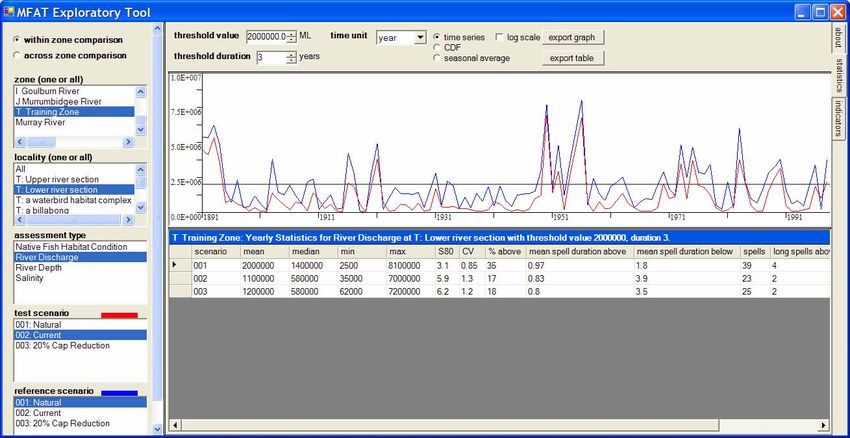
Figure 9.1 Example of within zone comparison, time series graph ............................................ 54
Figure A.1 .NET Licence agreement form .......................................................................... 60
Figure A.2 Content of mfat.ini configuration file ................................................................. 61
Figure C.1 MFAT conceptual linkages map ......................................................................... 68
Figure C.2 Floodplain vegetation habitat assessment model conceptual map ............................... 69
Figure C.3 Wetland vegetation habitat assessment model conceptual map .................................. 70
Figure C.4 Waterbird habitat assessment model conceptual map ............................................. 71
Figure C.5 Native fish habitat assessment model conceptual map............................................. 72
Figure C.6 Algal growth model conceptual map................................................................... 73
Tables
Table 1.1 Association between ecological models and locality types ...........................................4
Table 7.1 Woody Debris (WD) classes with default index values ............................................... 41
Table 7.2 Fish Passage (FP) classes with default index values.................................................. 41
Table 7.3 Water Temperature (WT) classes with default index values........................................ 41
Table 7.4 Look-up table of Channel Condition (CC) default index values..................................... 42
Table 7.5 Channel Condition (CC) index reduction factors and default values .............................. 42
Table 7.6 Spawning habitat condition (SHC) and larval habitat condition (LHC) definitions by fish group43
Table 7.7 Spawning habitat condition (SHC) and larval habitat condition (LHC) index names and definitions
....................................................................................................................... 44
Table 7.8 Substrate condition (SC) classes and default values – for group 4 only ........................... 46
Table 7.9 Summary of data input and preference curves for native fish ..................................... 50
Table 8.1 Cell counts and algal index values ...................................................................... 52
Murray Flow Assessment Tool – a Technical Description, ©2003 CSIRO, CRCFE iiiMurray Flow Assessment Tool – a Technical Description, ©2003 CSIRO, CRCFE iv
1                                                                                          Introduction

1          INTRODUCTION
The Murray Flow Assessment Tool (MFAT) is a software tool for predicting the ecological
benefits/impact of different flow scenarios along the River Murray system. It was developed by
CSIRO Land and Water for the Cooperative Research Centre for Freshwater Ecology (CRC FE) under
contract to the Murray-Darling Basin Commission. The MFAT has been used to support the Scientific
Reference Panel, an expert panel established by the CRC FE to undertake an assessment of three
proposed environmental flow reference points for the Living Murray Initiative.

The structure and conceptualisation of the MFAT are largely based on the Environmental Flows
Decision Support System (EFDSS) developed by CSIRO Land and Water and Environment Canada,
with financial support from the Murray-Darling Basin Commission, Land and Water Australia (then
Land and Water Resources Research and Development Corporation), and Environment Australia
(Young et al., 1999).

The MFAT assesses the impact/benefits of different flow scenarios on the condition of physical
habitat for native fish, waterbirds and vegetation communities, and also assesses the growth of
algal blooms. The MFAT makes these ecological assessments using daily river flows as the primary
input data to a number of ecological models that are largely parameterized on the basis of expert
knowledge. The MFAT enables an objective and repeatable assessment, and also allows the
integration of these assessments across spatial scales ranging from a single locality, through river
zones, and up to the entire river system. The results from the MFAT can then be used to facilitate
an informed trade-off process between environmental and human flow requirements.

Murray Flow Assessment Tool – a Technical Description, ©2003 CSIRO, CRCFE                              1
1                                                                                                      Introduction

1.1          Content and purpose of this report
This document was produced as part of a contractual agreement between the Murray Darling Basin
Commission, the CRC for Freshwater Ecology and CSIRO Land and Water. It was compiled and
edited by Anthony Scott1 and Susan Cuddy2 based on materials prepared by Bill Young2, Susan
Cuddy, Anthony Scott and Bronwyn Rennie1 for the MFAT Procedure Manual, January 2003,
(superseded by this document) and documentation which accompanies the MFAT software.

Its purpose is to provide up-to-date information on the implementation of the ecological models in
MFAT, how to parameterize them and how to use the analysis tools provided as part of MFAT. It
contains updated information to that contained in Young et al. (1999) but does not replace it.

This documentation is based on MFAT v.1.4 released by CSIRO in August 2003.

1.2          Basic structure of the MFAT
The MFAT is a decision support system that can be used to assess the ecological impact/benefit of
different flow scenarios at various localities along the River Murray River, both in-channel and on
the surrounding floodplains and wetlands. For in-channel localities, the daily river flows are used
directly to predict the changes in fish habitat condition and algal growth. For floodplain and
wetland localities, a floodplain configuration is set up which uses the daily river flows to estimate
the timing and quantity of water reaching each floodplain or wetland. These results are then used
to predict the response from floodplain vegetation, wetland vegetation and waterbirds. After
setting up appropriate weightings, the MFAT Explore Tool can be used to analyse the results and to
integrate assessments within river zones, across river zones or across the entire river system.
Figure 1.1 shows the basic framework of the MFAT.

           Input                               Processing                    Output

                  External river                    MFAT floodplain                MFAT ecological
              hydrology model flow               hydrology model and              assessment indices
                 data (e.g. MSM-                 ecological assessment
                     Bigmod)                            models

                                         Figure 1.1 Basic framework of the MFAT

1.3          Software and hardware requirements
This section provides an overview of the system specifications of MFAT version 1.4.

Hardware
The MFAT runs on a PC platform under the MS Windows operating system using standard IBM PC
clone hardware with at least a Pentium II processor. A minimum disk space of 200 MB is required
although this is dependent on the number of flow scenarios and localities being assessed. As an
example, a set of training databases (three flow scenarios and three floodplain configurations)
required about 30 MB. A minimum of 128 MB RAM and a 800 x 600 pixel screen resolution are
recommended.

1
    CRC for Freshwater Ecology
2
    CSIRO Land and Water, Canberra Lab

Murray Flow Assessment Tool – a Technical Description, ©2003 CSIRO, CRCFE                                        2
1 Introduction Software The MFAT has been developed using two different programming languages. This has come about because much of the MFAT is based on revisions to the EFDSS, for which total reprogramming could not be justified. The older components of the MFAT are written in MS Visual Basic and use the underlying RAISONTM software (developed by Environment Canada). These need some Visual Basic controls (*.VBX) and some components of the RAISONTM software to be installed. These are distributed with the software. The rewritten (and new) components are coded in C# in the Microsoft .NET environment. The .NET framework is compatible with Windows operating systems ’98, 2000, NT, and XP. The software is distributed in a zip file. The contents of this file, and install instructions, are documented in Appendix A to this Report. Supporting software Microsoft .NET, Microsoft MDAC (data access components) and JET. These are available under free distributable licenses from Microsoft and are provided on the MFAT installation disk. Depending on the configuration of your computer, you may need to install none or all of these. The original EFDSS was developed using tools from the RAISONTM for Windows Decision Support System (Lam et al., 1994). A licensed copy of RAISONTM is also required to run some components of the read-write version of MFAT. RAISONTM licenses for MFAT can be obtained from the Murray- Darling Basin Commission under a special agreement with the National Water Research Institute, Environment Canada. 1.4 Databases All MFAT data are stored in Microsoft Access™ Version 2.0 databases. Conventions for key, date and time series fields have been implemented. For example, most time series data are stored in binary long object (BLOB) fields to reduce storage requirements. These fields, which cannot be viewed within Access, can be displayed using the MFAT Explore tool. Databases and their tables are detailed in Section B.2 of this Report. While CSIRO is responsible for the implementation of the models in MFAT, the databases were populated by the CRC FE and members of the Regional Evaluation Groups (REGs) established by the Murray Darling Basin Commission. Evidence, including references, supporting the data is contained in Evidence tables contained within the MFAT databases and in other documents produced as part of the Living Murray Initiative. A conceptual diagram of MFAT databases and their linkages is available at Figure C.1. 1.5 Ecological assessments, localities and zones Ecological assessments The MFAT allows users to investigate different flow scenarios and their likely ecological consequences for river and floodplain environments. Ecological consequences are divided into two categories: Murray Flow Assessment Tool – a Technical Description, ©2003 CSIRO, CRCFE 3
1                                                                                                                 Introduction

       1. The habitat condition assessment category includes assessments for native fish habitat,
          floodplain vegetation habitat, aquatic wetland vegetation habitat, and waterbird habitat.
       2. The nuisance assessment is an assessment of algal bloom occurrence.

Each of these single assessments (one ecological group assessed at one locality) can then be
integrated using the MFAT Explore Tool.

Localities
The MFAT recognises six locality types:

       •    river sections
       •    weir pools
       •    billabongs/lagoons
       •    riverine lakes
       •    floodplains
       •    waterbird habitat complexes.

The first two are ‘in-channel’ locality types, the remainder are ‘off-river’ locality types.

Hydrology data is associated with localities, and simulation models can only be run at these
localities. The in-river localities are described by hydrology data imported from an external
hydrology simulation model, such as MSM-BigMod or IQQM. Off-river localities are described by
hydrology data from the MFAT floodplain hydrology model. The hydrology data drives the
assessment models at the different localities.

Details of locality types and a record of which assessments (or models) are run at each locality are
stored in database tables which are defined during the MFAT setup process. Each run of an
assessment model is for a single flow scenario at a single locality.

The ecological assessment models are associated with particular locality types (Table 1.1).

                            Table 1.1 Association between ecological models and locality types

    Assessment Model           MFAT Locality Type            Hydrology Data

    Native Fish Habitat        ‘River Sections’              Each MFAT ‘river section’ locality is linked to a river node.
    Condition                                                Daily flow for each scenario and stage height data are
                                                             provided for each river node by an external river hydrology
                                                             model.

    Floodplain Vegetation      ‘Floodplains’                 The Floodplain Hydrology Model is used to describe ‘off-
    Habitat Condition                                        river’ hydrology. The floodplain configuration is linked to a
                                                             river node (flow file) to receive its initial inflow.

    Wetland Vegetation         ‘Riverine lakes’              The MFAT Floodplain Hydrology Model is used to describe
    Habitat Condition          ‘Billabongs/lagoons’          ‘off-river’ hydrology. The floodplain configuration is linked
                                                             to a river node (flow file) to receive its initial inflow.

    Waterbird Habitat          ‘Waterbird habitat complex’   The MFAT Floodplain Hydrology Model is used to describe
    Condition                                                ‘off-river’ hydrology. The floodplain configuration is linked
                                                             to a river node (flow file) to receive its initial inflow.

    Algal Growth Model         ‘Weir Pools’                  Each MFAT ‘weir pool’ locality is linked to a river node
                                                             (flow file). Daily flow for each scenario and stage height
                                                             data are provided for each river node by an external river
                                                             hydrology model.

Murray Flow Assessment Tool – a Technical Description, ©2003 CSIRO, CRCFE                                                    4
1 Introduction
Zones
Localities are grouped into river zones to enable spatial integration. Zones have been mapped to
the ten (10) River Murray reaches that have been defined for the Living Murray Initiative, and are
shown in Figure 1.2.
Zone F
Zone E
Zone J: Murrumbidgee
Zone G Zone D
Zone B
Zone C
Zone H
Zone A
Zone I: Goulburn
Figure 1.2 The ten zones along the River Murray System, being assessed using the MFAT as part of the Living
Murray Initiative
1.6 Flow scenarios used in the MFAT
Within MFAT, a scenario is a set of daily flow records for selected river locations. There is no limit
to the number of scenarios that can be loaded into the MFAT, except for any data storage
constraints of the hardware being used. Clearly, large numbers of scenarios will increase
processing and data access times. It is suggested that between 4 and 12 scenarios is sufficient to
allow investigation of a wide range of alternative flow options. Extra scenarios can be loaded into
the system at any time.
The MFAT recognises two special scenarios that are assumed to always be in the set of scenarios −
the ‘natural’ scenario, and the ‘current‘ scenario. The natural scenario is the flow conditions
without flow regulation or diversion. This means no water management infrastructure − for
example, dams − and no irrigation or other consumptive water use. Typically, it does not include
natural land use conditions, as the data to allow calibration of a river hydrology model to pre-
catchment disturbance conditions are seldom available. The current scenario is the flow conditions
under the present level of development − land use, regulation and diversions.
Importantly, it is sensible for flow scenarios to be of the same length, eg 100 years of daily flow.
This ensures consistency of prediction and comparison of alternate scenarios. These flow records
can be provided by any river hydrology model, as long as the output is a file of daily flow values
which can be imported into MFAT.
Murray Flow Assessment Tool – a Technical Description, ©2003 CSIRO, CRCFE 51 Introduction MSM-BigMOD and IQQM For localities along the River Murray and lower Darling, the flow files for each scenario are provided by the MSM-BigMOD model, which has been developed by the MDBC. The model is complex and includes rainfall-runoff relationships, operating rules for storages, irrigation demands, water resource assessment and water accounting, and flow and salinity routing. MSM-BigMOD provides daily flows for a period of over 100 years. The flow series for each locality (or river flow node) are provided as a file which can be imported into the MFAT. The IQQM model, developed by the NSW Department of Infrastructure, Planning and Natural Resources (previously Land and Water Conservation) (Podger et al., 1994) provided the flow files for the Murrumbidgee River. A similar model provided flow files for the Goulburn River. 1.7 Read-only (‘public’) and read-write (‘restricted’) modes The distributable version of MFAT is v1.4 which provides a read-only (public) mode for public distribution and a read-write (restricted) mode for licensed users. MFAT defaults to running in public mode. To run MFAT v1.4 in read-write mode, a separate MFAT control program is required. This is available through the Commission, and its distribution is restricted by licence. The only difference between the modes is that, in read-only mode, all databases are fully populated and the Run and Save buttons in the user interface are disabled. ‘Fully populated databases’ means that all models have been run and databases updated with run results. In public mode, you can view, but not alter, all data in the system. This includes input data, as well as run results. Disabled means that the buttons are either greyed out, or simply not displayed, depending on the context. In the read-write mode, users can add/edit all input data, and run the assessments to populate the databases. Murray Flow Assessment Tool – a Technical Description, ©2003 CSIRO, CRCFE 6
2                                                                                 The Floodplain Hydrology Model

2          THE FLOODPLAIN HYDROLOGY MODEL
The MFAT includes a model for configuring and running simulations of floodplain hydrology. The
model represents the floodplain system as a network of storages and pipes. The floodplain
hydrology model provides a time series of daily volume for each storage, in the same way as the
external river hydrology model provides a time series of daily flow for a river section. In fact, the
floodplain hydrology model is driven by flow data provided by the external river hydrology model.

The model allows very simple or very complex configurations to be defined. The level of
complexity should reflect both the actual complexity of the floodplain system, and also the extent
of data available to accurately parameterise the model.

2.1        Elements of a floodplain configuration
A floodplain configuration is a set of storages which are linked by (conceptual) pipes. A simple
example of a floodplain configuration is shown in Figure 2.1. The configuration must be defined
before its storages and pipes can be created. A configuration must be linked to a ZONE to pick up
the correct potential evapotranspiration (PET) data. This is provided in the Configuration
‘Properties’ dialog box.

           Figure 2.1 Floodplain hydrology model interface showing a simple floodplain configuration

Murray Flow Assessment Tool – a Technical Description, ©2003 CSIRO, CRCFE                                     7
2 The Floodplain Hydrology Model
Storages
Storages are elements on the floodplain which periodically receive water from the river. They are
assigned one of the following types:
• (used for special case of partitioning storage, ref below)
• floodplain
• billabong/lagoon
• riverine lake.
They are parameterised with
• maximum area
• maximum storage volume
• initial storage volume
• area-volume relationship
• (seepage) decay rate.
At each time step (t) the floodplain model calculates the volume (V) in a storage according to the
water balance of Equation 2.1, in terms of the pipe inflows (I), pipe outflows (O), the evapo-
transpiration rate (ET) across the inundated area (A), and the seepage rate (k).
Vt = (Vt −1 + I t − Ot − ETt × At −1 ) × e kt 2.1
Pipes
Storages are linked to the river and to each other via (conceptual) pipes. These pipes both feed
water to a storage and drain water away from it.
Most pipes are parameterised with
• Pmin – the volume in the source storage at which the pipe commences to flow
• Pmax – the volume in the source storage that coupled with Pmin defines the pipe capacity, vis
capacity = Pmax – Pmin
A special class of pipe – a ‘return pipe’ – has no parameters and is described in the following
section.
2.2 MFAT floodplain constructs
Storages and pipes can be parameterised to describe many types of behaviour that are observed on
the floodplain. Special storage constructs have been developed for MFAT to describe
• partitioning flow from the river onto the floodplain
• fully shedding floodplains
• partially shedding floodplains
• multi-level shedding floodplains
• floodplain wetlands.
Details on how to use and parameterize these storages, and extra information on how to establish
the volume area relationships and decay rate parameters, are below.
Murray Flow Assessment Tool – a Technical Description, ©2003 CSIRO, CRCFE 82 The Floodplain Hydrology Model
Pipe constructs have been developed to describe
• moving water between storages
• draining shedding floodplains (called ‘return’ pipes).
These are also described below.
River flow partitioning pipe and storage
If the river hydrology model does not provide flow to the floodplain, it is necessary to calculate this
from channel flow. A simple construct for doing this is to set up a ‘partitioning’ storage to
calculate the split between overbank flow reaching the floodplains and wetlands, and channel flow
that continues down the main river channel.
To do this requires the construction of a storage with one input and multiple output pipes as
follows:
1. a storage (of type ) of zero volume and zero decay rate
2. an input pipe to the storage whose flow is taken from a times series of river flow provided by a
floodplain hydrology model
3. an output pipe from the storage that does not connect to another storage (notionally returns to
the river) with a Pmin of zero and a Pmax that exceeds the highest flow ever experienced in that
part of the river
4. any number of other output pipes that connect to other floodplain and wetland storages. Each
pipe is set as follows
• set the Pmin to the ‘Commence to Flow’ (CTF) for the floodplain or wetland storage
• set the Pmax so that the peak flow reaching the storage is equal to Pmax - Pmin.
Fully shedding floodplains
For a floodplain whose water level rises and falls directly with the river water level (and has no lag
and hence no ‘storage’ behaviour) use a ‘return pipe’ to drain all of yesterday’s water back to the
river, so that today’s storage volume is equal to today’s inflow.
If the water level on the floodplain does not respond immediately to the water level in the river
(and has a lag), but does eventually shed all water, a ‘standard’ pipe should be used for the output,
with a Pmin of zero. This allows all water to drain off the floodplain. The pipe capacity (Pmax – Pmin )
will vary according to how rapidly the floodplain drains.
Partially shedding floodplains
Partially shedding floodplains (some water is retained on the floodplain after the flood recedes)
have one or more output pipes but with Pmin greater than zero, again with capacity reflecting rate
of drainage. Complete drying in this case occurs through seepage (via the ‘decay rate’) or by
evapotranspiration.
Murray Flow Assessment Tool – a Technical Description, ©2003 CSIRO, CRCFE 92 The Floodplain Hydrology Model
Multi-level shedding floodplains
To represent multi-level floodplains that occur as successive benches above the channel, link each
successive higher level floodplain to the previous level floodplain using a single pipe. Higher level
floodplain storages may have a ‘return pipe’ if they drain rapidly, and/or may have other ‘drain’
pipes that drain water more slowly.
Floodplain wetlands
Billabongs/lagoons, and riverine lakes are defined as ‘floodplain wetlands’ in MFAT, and may be
represented by one or more storage elements.
Floodplain wetland storages may have one or more ‘slow’ (low capacity) drain pipes, but probably
with Pmin well above the empty storage level. The output pipe capacity is determined by Pmax – Pmin.
These wetlands may empty by evaporation, or may also have a decay rate that increases the loss
rate and represents drainage to groundwater.
Volume-Area Relationships
Each storage requires a volume-area relationship. This describes how the inundated area changes
with storage volume. The volume-area relationship also defines the average depth of the storage
(average depth = volume/area). The inundated area and the average depth are used in the
waterbird habitat, floodplain vegetation habitat and wetland vegetation habitat condition models.
Volume-area curves should include some data points close to the origin to ensure that sensible
depths are obtained for storages which are almost dry.
Volume-Area relationships will range from those for relatively steep ‘U’ cross-section billabongs
which, as they drain or dry out, have a loss in volume with almost no loss in area (Figure 2.2), to
wide, shallow riverine lakes formed in aeolian deflation basins, where initial drainage causes losses
in both area and volume (Figure 2.3).
Billabong
60 4.5
4
50
3.5
40 3
mean depth (m)
Area (Ha)
2.5
30
2
20 MFAT volume-area curve 1.5
1
10 MFAT calculated mean
depth* 0.5
0 0
0 500 1000 1500 2000 2500
Volume (ML)
Figure 2.2 Suggested volume-area relationship for ‘U’ cross-section billabong
Murray Flow Assessment Tool – a Technical Description, ©2003 CSIRO, CRCFE 102 The Floodplain Hydrology Model
Lake
120 1.20
100 1.00
80 0.80
mean depth (m)
Area (Ha)
60 0.60
40 0.40
MFAT volume-area curve
20 0.20
MFAT calculated mean depth*
0 0.00
0 200 400 600 800 1000
Volum e (ML)
Figure 2.3 Suggested volume-area relationship shape for wide shallow riverine lake
More unusual storages include those where the average depth increases as they drain. This could
occur for a waterhole with a deep central channel and a wide shallow margin. In this case the
average depth will initially increase on draining, but then, once the central channel section begins
to drain, the average depth will decrease.
Ideally, volume-area relationships would be established using cross-sectional survey information.
However, knowledge of the typical cross-sectional shape is generally sufficient to represent the
changes in inundated area with filling and draining.
Decay Rate
Storages are parameterised by an exponential decay rate (k). This is used to represent the rate at
which water is lost to groundwater. Negative values are required to produce a loss (Equation 2.1).
Realistic rates will depend on the soil type and the nature of underlying aquifers. Typically values
are probably between –0.002 and –0.02, which represent loss rates of 0.2% and 2% respectively, per
day.
Moving water between storages
For floodplain or wetland storages that are not fed by partitioning storages, their inflow pipe is set
as follows;
• Set the Pmin at the level in the supply storage at which the connected storage commences to
fill with water. For example, if storage A, the ‘supply’ storage, (max volume 1000 ML) starts
to flow into storage B, the connected storage, when it is 50% full, then set the P min of the
inflow pipe to storage B to 500ML.
• Set the Pmax so that the peak flow reaching the new storage is equal to Pmax - Pmin . Note that
Pmax should be less than the maximum volume of the supply storage.
Murray Flow Assessment Tool – a Technical Description, ©2003 CSIRO, CRCFE 112 The Floodplain Hydrology Model
‘Return pipes’
A return pipe is a special case of a pipe which is used to represent the rapid drainage of water from
shedding floodplains directly back to the river – essentially a return pipe drains the storage in a
single time step (day) once the river flow drops. Return pipes have no parameters.
For return pipes, the water balance of Equation 2.1 uses Ot = Vt −1 and hence the water balance for
the source storage becomes simply that of Equation 2.2.
Vt = (I t − ETt × At −1 ) × e kt 2.2
2.3 Procedural guide for setting up a floodplain configuration
The suggested procedure for setting up a floodplain configuration is outlined below.
Step 1 – draw a mud map
Produce a ‘mud map’ of the floodplain-wetland system, and identify floodplains (water shedding
areas), wetlands (water holding areas), and connecting channels (water moving areas). Identify
inflow and outflow pathways for these areas.
Step 2 – specify storages for assessment
Decide which storage elements of the system you wish to use to represent waterbird habitat,
floodplain vegetation habitat or wetland vegetation habitat. (Consider elements with national or
international significance, elements which are representative of the region, and elements which
contain the best hydrological and ecological data).
Step 3 – specify other storages
Determine if there are any connecting storage elements within the system that must also be
modelled to provide accurate hydrological inputs to the storage elements identified in (2).
Step 4 – record properties for each storage
Record the following data (and the references) for each storage element.
• (a) storage type (floodplain, riverine lake, billabong/lagoon)
• (b) number of connecting channels or pathways to river (a pathway might include overbank
sheet flow). Each pathway will be modelled by a separate ‘pipe’
• (c) maximum area in hectares of the storage element
• (d) maximum volume in ML (for a floodplain storage this will be defined by the largest flood
recorded)
• (e) initial volume in ML. This will be 0 ML for a dry wetland and some other value for an
already wet wetland. (This value is only used in the initial year of computation, and in most
cases only affects the results for year 1.)
• (f) commence to flow (ML/day) in river when water flows along pathway (or pipe) into the
storage element; and the river node which provides the in-stream flow data
• (g) maximum capacity of this pathway (ML)
• Repeat (f) and (g) for all inlet pathways to the storage element
• (h) volume in storage element when outflow commences to flow, and when it ceases to flow
Murray Flow Assessment Tool – a Technical Description, ©2003 CSIRO, CRCFE 122 The Floodplain Hydrology Model
• (i) return flow limit (water being moved back to the river system) in ML/day
• (j) volume-area relationship
• (k) average flood frequency and duration. Also record any other flooding data that might help
calibrate the model.
Example configuration
Figure 2.4 is an example of a floodplain configuration. The configuration has a partitioning storage
construct to determine overbank flow from the river, has two shedding floodplains at different
levels, both with return pipes, and a riverine lake that receives water from the higher floodplain
level.
Figure 2.4 Example floodplain configuration
The lake is notionally contained within the higher floodplain, and receives water shortly after the
floodplain is about 40% (by volume) inundated. The lake has no outlet pipe and loses water only by
evapotranspiration (ET) and decay (groundwater seepage).
(The floodplain model only allows inflows from the left of the edit window. This means that connections
must be drawn from the left, irrespective of which side of the river the system lies. For systems that have
elements on both sides of the river, these two parts of the system would be drawn one above the other.)
Running the model3
The command Run gives you the ability to run the configuration for one or all (flow) scenarios. The
Batch Run button will run all scenarios for all configurations.
3
Running the model is only available to those with MFAT read-write mode. For all others, the Run and Batch Run buttons
are not available (they are disabled and greyed out).
Murray Flow Assessment Tool – a Technical Description, ©2003 CSIRO, CRCFE 132 The Floodplain Hydrology Model
Both Run and Batch Run take the daily inflow data (provided by the external river hydrology
model) and then run it through the configurations of storages and pipes to produce daily time series
of volumes in the pipes and storages.
Analysing results
The simulated volume time series for pipes and storages can be viewed by selecting Pipe Graph or
Storage Graph.
Figure 2.5 Examples of Pipe Flow Volume and Storage Volume graphs of daily volumes
The Storage Volume graph gives access to time series of the storage’s daily volume and its daily
area (via the radio buttons in the bottom left hand corner of the graph window). Time series for all
scenarios can be visualized by selecting the scenario from the scenario list at the bottom of the
graph window. (Hint: Positioning the mouse over the right arrow of the year bar and double clicking will
automatically move through the time series.)
Calibration of the floodplain configurations
For each storage element, the simulated volume (and area) time series should be compared with
field data and anecdotal knowledge of the flooding and drying patterns experienced by that
storage. This will include a comparison of parameters such as;
• flood frequency
• flood duration
• flood magnitude (volume and area inundated)
• typical length of dry periods
• rate of drainage after flood recession
Murray Flow Assessment Tool – a Technical Description, ©2003 CSIRO, CRCFE 142 The Floodplain Hydrology Model
• rate of rise during floods.
Fine tuning of model response can be achieved by adjusting;
• inlet pipe properties (Pmin and Pmax) to adjust the rate of filling and the commence to flow
• outlet pipe properties (Pmin and Pmax) to adjust the rate of draining and the cease to flow
volume
• decay rates (or groundwater seepage)
• maximum storage volumes and areas, and the area-volume graphs
• the number of input and output pipes connected to each storage.
Murray Flow Assessment Tool – a Technical Description, ©2003 CSIRO, CRCFE 153 MFAT Ecological Assessment Models
3 MFAT ECOLOGICAL ASSESSMENT MODELS
The MFAT contains five ecological models. The first four models assess habitat condition under
different flow scenarios for;
• native fish
• floodplain vegetation
• aquatic wetland vegetation
• waterbirds.
The fifth model is an assessment of Algal Growth (rather than habitat condition).
The first four ecological models rely on user-defined ‘preference curves’ to determine the output
indices.
3.1 Preference Curves
X-axis
A preference curve has as its x axis (or input) a variable that is usually a function of the flow
regime (a hydrologic or hydraulic variable) or a function of time (such as calendar month, or time
duration – usually days or months). Some of the preference curves used in the models are functions
of:
• daily water depth
• daily depth variability for the year
• flow percentile
• rate of depth increase
• duration of rate of depth increase
• rate of depth decrease
• duration of dry period between inundation
• percentage of total area inundated
• duration of inundation
• calendar months for spawning.
Most of the preference curves describe the response of a particular biotic group to environmental
conditions. In addition to varying between groups these responses may also vary between
localities. For example, not only may Golden perch have a different preferred season for spawning
to Freshwater catfish, Golden perch in the lower Darling may have a different preferred season for
spawning than Golden perch in the Murray near Yarrawonga.
Details of how to set individual preference curves will be considered in following sections, model by
model.
Y-axis
A preference curve has as its y axis (or output) a non-dimensional index with a range from 0 to 1.
Zero (0) is used to indicate intolerable habitat conditions, and one (1) is used to indicate ‘ideal’
habitat conditions. The index value of one (1) is not necessarily related to the ‘natural’ flow
Murray Flow Assessment Tool – a Technical Description, ©2003 CSIRO, CRCFE 163 MFAT Ecological Assessment Models
conditions, because it is recognised that while natural could be considered ecologically optimal for
the entire system, the natural flow condition does not provide ideal habitat for all biota at all
times.
Figure 3.1 Preference curve for spawning timing of ‘flood spawners’
3.2 Weights
MFAT uses weights within, between and across assessment models to indicate the relative
importance of different aspects of the assessment.
At the assessment model level4, weights are used to indicate the relative importance of
• life cycle stages
• each criterion within each stage.
Examples from the waterbird habitat assessment model are the relative importance of
• breeding habitat and foraging habitat to the overall waterbird habitat condition
assessment
• flood duration, rate of fall, dry period and nesting vegetation to the breeding habitat
condition assessment.
External to the assessment model,5 weights indicate the relative importance of:
• different zones along the river
• assessment models for each zone
• localities within each zone, by assessment model
• groups and/or communities within each assessment at each locality.
4
These weights are set and viewed within each assessment model.
5
These weights are set and viewed using the MFAT Set up Weights tool.
Murray Flow Assessment Tool – a Technical Description, ©2003 CSIRO, CRCFE 173 MFAT Ecological Assessment Models
Figure 3.2 Weights window showing zone, zone-assessment, locality-assessment and assessment group weights
for native fish at Upper Mitta river locality within Zone A. Note that these are not necessarily the weightings
used in the Living Murray Initiative assessment.
The form shown in Figure 3.2 demonstrates how these weights are set.
Weights may reflect some or all of the following factors:
• amount or quality of information underpinning each component of the assessment
• relative extent (length or area) represented by the locality
• ecological importance of the species group or locality to the overall community structure
• conservation status of the particular group or locality
• icon status of the particular group or locality
• national or International significance of a particular group or locality
• indigenous interests
• local community or stakeholder group interests or values.
As with other data that is entered into MFAT, a facility is provided for users to record the
‘evidence’ or justification for the weights that are entered.
Murray Flow Assessment Tool – a Technical Description, ©2003 CSIRO, CRCFE 183 MFAT Ecological Assessment Models
Setting weights
There is no prescription for setting weights. Indeed, they can all be set the same, ie each
criterion, life cycle stage, assessment, locality and zone can have equal weighting. Weights are
entered as integers. These values are normalised to being between 0 and 1 by MFAT and the
entered values, and their normalised weights, are displayed.
Note that the overall assessments made by the MFAT Explore tool are integrated across all groups
for a given assessment model. To take advantage of Explore to investigate statistics and indicators
for a single group within an assessment model where several groups have been run, it is necessary
to use weights of zero to ‘turn off’ the groups that are not of interest. This is only available to
those with MFAT read-write mode.
3.3 Recording evidence
MFAT provides a simple mechanism (Figure 3.3) for recording the quality and source of ecological
data and information that is used to assign preference curves and weightings. Four pieces of
‘evidence’ are recorded:
• author
• date of entry
• confidence level
• evidence and sources of information.
Figure 3.3 Form for recording evidence
A confidence level must be assigned to each piece of evidence. Three (3) levels are provided:
• (A) Expert judgement supported by data and consensus knowledge from published
papers and reports
Murray Flow Assessment Tool – a Technical Description, ©2003 CSIRO, CRCFE 193 MFAT Ecological Assessment Models
• (B) Expert judgement supported by unpublished data or knowledge that can be made
available for public consideration
• (C) Expert judgement based on general scientific experience or anecdotal information.
The user who has entered the data will have made an appropriate selection from the Confidence
Level list.
The ‘Evidence’ and ‘Sources’ boxes are MEMO fields which mean they have no limit on their length.
In the case of preference curves, two sets of evidence are recorded and available for viewing. One
is associated with the default values provided by the Scientific Reference Panel (SRP), and are
accessed via the SRP Evidence button. The other, to record evidence supporting any changes to the
default values, is available via the standard Evidence button.
Murray Flow Assessment Tool – a Technical Description, ©2003 CSIRO, CRCFE 204 The Floodplain Vegetation Habitat Condition Model
4 THE FLOODPLAIN VEGETATION HABITAT CONDITION MODEL
4.1 Model development
The MFAT floodplain vegetation habitat condition (FVHC) model is a refinement of the Vegetation
Habitat Condition (VHC) model of the EFDSS (Young et al., 1999). The EFDSS VHC model was
based primarily on information obtained via formal interviews with Leon Bren, Terry Hillman, Jane
Roberts, Alistar Robertson, Geoff Sainty and Glen Walker in 1996. These conceptualisations are
documented in Young et al. (1999), Roberts (2001) and diagrammatically in Appendix C, Figure C.2.
The refinements that led to the FVHC were primarily based on interviews with Jane Roberts and Terry
Hillman in 2002-3, and were reviewed and endorsed for use in MFAT v1.4 by the Scientific Reference
Panel of the Living Murray Initiative. Evidence supporting the MFAT input data is recorded in the
Evidence tables in the FVEGHAB database for each zone. This evidence has been prepared by the
CRC FE and regional evaluation groups.
4.2 Model description
The FVHC model enables simulation of the likely condition of floodplain vegetation habitat
(primarily flow-related habitat) on the floodplains of the Murray River system under different river
flow scenarios. The model is run for ‘floodplains’ for which the hydrology can reasonably be
described by time series data of inundation volumes and inundation areas. Other input data are in
the form of habitat preference curves that relate aspects of habitat condition to hydrologic,
hydraulic or time variables.
Habitat condition is represented by a dimensionless ‘unit’ index that ranges from 0 (intolerable) to
1 (ideal). Ideal is not considered equivalent to natural, the latter usually being less than ideal for
the long term average. Explicit consideration is made of adult and recruitment (specifically
germination and seedling establishment) habitat preferences, with habitat condition indices
calculated for each life stage.
Vegetation groups
Separate assessments are made for five (5) vegetation groups
• River red gum forest
• River red gum woodland
• Black box woodland
• Lignum shrubland
• Rats Tail Couch grassland/
4.3 Habitat condition indices
The annual floodplain vegetation habitat condition index (FVHC) is a weighted sum of an annual
adult habitat condition index (AHC) and an annual recruitment habitat condition index (RHC)
(equation 4.1). The annual values of FVHC, AHC and RHC are for a water year (July-June).
FVHC = x1AHC + x2RHC 4.1
where xi are normalised weights that are defined for each vegetation group.
Murray Flow Assessment Tool – a Technical Description, ©2003 CSIRO, CRCFE 214 The Floodplain Vegetation Habitat Condition Model
4.4 Adult Habitat Condition (AHC) indices
Adult habitat condition (AHC) is a function of unit indices for flood timing (FT), inundation duration
(FD), annual drying period (DP) and flood memory (FM). A preliminary value of AHC (AHC*) is
calculated as a function of FT, FD and DP (equation 4.2).
AHC* = 3 FT ∗ FD ∗ DP 4.2
FM is partly a function of AHC*. The final AHC is then a function of FT, FD, DP and FM (equation
4.3).
AHC = 4 FT ∗ FD ∗ DP ∗ FM 4.3
FT, FD, DP and FM are all determined by preference curves which are specific to vegetation group,
but do not vary between localities. FM is also partly determined by 4 separate parameters, all of
which are vegetation group specific.
Flood Timing (FT)
FT values are determined by a preference curve that indicates the relative preferability of the
different calendar months for the timing of inundation of the floodplain (for the maintenance of
adult vegetation). The preference curve is treated as a continuous function not a stepwise monthly
function6. Daily FT values are therefore interpolated from the preference curve according to the
position within a calendar month.
The annual value of FT for a water year is the median of
the daily values over the duration (see Inundation
Duration) of the ‘best flood event’. The ‘best flood
event’ is the event that produces the highest value of
AHC*.
Inundation Duration (FD)
FD values are determined by a preference curve that indicates the preferred duration (in days) of
floodplain inundation (for the maintenance of adult vegetation).
The annual value of FD for a water year is the single value from
the preference curve for the ‘best flood event’, with the
duration of the event being defined as the period for which the
inundated area exceeds 50% of the total floodplain area.
Note: This definition of an inundation event means that, the
volume-area relationships defined for the floodplain in the floodplain hydrology model will affect
the FVHC model outputs.
Inter-flood Dry Period (DP)
DP values are determined by a preference curve that indicates the preferred duration (in months)
of the dry period since the last flood.
6
Sample graphs are provided with each preference curve as a visual aid to support the description of curve definition in this
report. They are not necessarily endorsed by the authors or the Scientific Reference Panel.
Murray Flow Assessment Tool – a Technical Description, ©2003 CSIRO, CRCFE 22You can also read