Multistep-ahead daily inflow forecasting using the ERA-Interim reanalysis data set based on gradient-boosting regression trees
←
→
Page content transcription
If your browser does not render page correctly, please read the page content below
Hydrol. Earth Syst. Sci., 24, 2343–2363, 2020
https://doi.org/10.5194/hess-24-2343-2020
© Author(s) 2020. This work is distributed under
the Creative Commons Attribution 4.0 License.

Multistep-ahead daily inflow forecasting using the ERA-Interim
reanalysis data set based on gradient-boosting regression trees
Shengli Liao1,2 , Zhanwei Liu1,2 , Benxi Liu1,2 , Chuntian Cheng1,2 , Xinfeng Jin1,2 , and Zhipeng Zhao1,2
1 Institute
         of Hydropower System and Hydroinformatics, Dalian University of Technology, Dalian 116024, China
2 KeyLaboratory of Ocean Energy Utilization and Energy Conservation of Ministry of Education,
Dalian University of Technology, Dalian 116024, China

Correspondence: Zhanwei Liu (337891617@qq.com)

Received: 13 November 2019 – Discussion started: 13 December 2019
Revised: 10 March 2020 – Accepted: 8 April 2020 – Published: 8 May 2020

Abstract. Inflow forecasting plays an essential role in reser-   cate that reanalysis data enhance the accuracy of inflow fore-
voir management and operation. The impacts of climate            casting for all of the lead times studied (1–10 d), and the
change and human activities have made accurate inflow            method developed generally performs better than other mod-
prediction increasingly difficult, especially for longer lead    els, especially for extreme values and longer lead times (4–
times. In this study, a new hybrid inflow forecast frame-        10 d).
work – using the ERA-Interim reanalysis data set as input
and adopting gradient-boosting regression trees (GBRT) and
the maximal information coefficient (MIC) – is developed for
                                                                 1   Introduction
multistep-ahead daily inflow forecasting. Firstly, the ERA-
Interim reanalysis data set provides more information for        Reliable and accurate inflow forecasting 1–10 d in advance
the framework, allowing it to discover inflow for longer lead    is significant with respect to the efficient utilization of wa-
times. Secondly, MIC can identify an effective feature sub-      ter resources, reservoir operation and flood control, espe-
set from massive features that significantly affects inflow;     cially in areas with concentrated rainfall. Rainfall in southern
therefore, the framework can reduce computational burden,        China is usually concentrated for several days at a time due to
distinguish key attributes from unimportant ones and pro-        strong convective weather, such as typhoons. Low accuracy
vide a concise understanding of inflow. Lastly, GBRT is a        inflow predictions can consequently mean that power sta-
prediction model in the form of an ensemble of decision          tions are unable to devise reasonable power generation plans
trees, and it has a strong ability to more fully capture non-    7–10 d ahead of disaster events, and this subsequently leads
linear relationships between input and output at longer lead     to unnecessary water abandonment and even substantial eco-
times. The Xiaowan hydropower station, located in Yunnan         nomic losses. Figure 1 shows the “losses of electric quantity
Province, China, was selected as the study area. Six evalu-      due to discarded water” (LEQDW) in Yunnan and Sichuan
ation criteria, namely the mean absolute error (MAE), the        provinces, China, from 2011 to 2016 (Sohu, 2017; Jiang,
root-mean-squared error (RMSE), the Pearson correlation          2018). The total LEQDW in Yunnan and Sichuan provinces
coefficient (CORR), Kling–Gupta efficiency (KGE) scores,         increased from 1.5 × 10⁹ to 45.6 × 10⁹ kWh during the pe-
the percent bias in the flow duration curve high-segment vol-    riod from 2011 to 2016, with an average annual growth rate
ume (BHV) and the index of agreement (IA) are used to eval-      of 98.0 %. In recent years, due to the increasing number of
uate the established models utilizing historical daily inflow    hydropower stations and improved hydropower capacity, the
data (1 January 2017–31 December 2018). The performance          problem of discarding water due to inaccurate inflow fore-
of the presented framework is compared to that of artificial     casting is becoming increasingly serious and has had a nega-
neural network (ANN), support vector regression (SVR) and        tive impact on the development of hydropower in China.
multiple linear regression (MLR) models. The results indi-

Published by Copernicus Publications on behalf of the European Geosciences Union.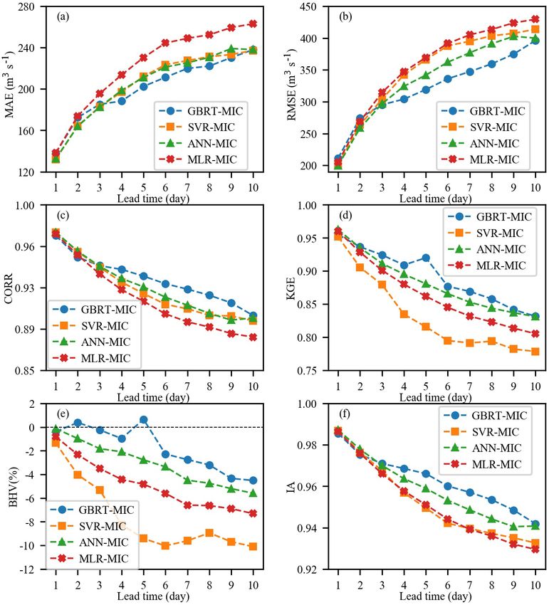
2344                                                    S. Liao et al.: Daily inflow forecasting using ERA-Interim reanalysis

   The main challenge with respect to inflow forecasting at        2019) issues, where it has proven to alleviate the above-
present, which is caused by climate change and human ac-           mentioned problems. Thus, GBRT is selected for daily inflow
tivities, is low accuracy, especially for longer lead times        prediction with lead times of 1–10 d in this paper. Compared
(Badrzadeh et al., 2013; El-Shafie et al., 2007). Meanwhile,       with ANN and SVR, GBRT also has two other advantages.
streamflow variation, which also stems from climate change         Firstly, GBRT can rank features according to their contribu-
and anthropogenic activities, means that inflow forecasting        tion to model scores, which is of great significance for re-
models often need to be rebuilt, and the model parameters          ducing the complexity of the model. Secondly, GBRT is a
need to be recalibrated according to the actual inflow and         white box model and can be easily interpreted. To the best of
meteorological data within 1 or 2 years.                           our knowledge, GBRT has not previously been used for daily
   To address these problems, a variety of models and ap-          inflow prediction with lead times of 1–10 d. For comparison
proaches have been developed. These approaches can be              purposes, ANN, SVR and multiple linear regression (MLR)
divided into three categories: statistical methods (Valipour       have been employed to forecast daily inflow and are consid-
et al., 2013), physical methods (Duan et al., 1992; Wang           ered to be benchmark models in this study.
et al., 2011; Robertson et al., 2013) and machine-learning            In addition to forecasting models, a vital reason why many
methods (Chau et al., 2005; Liu et al., 2015; Rajaee et al.,       approaches cannot attain a higher inflow prediction accuracy
2019; Zhang et al., 2018; Yaseen et al., 2019; Fotovatikhah        is that inflow is influenced by various factors (Yang et al.,
et al., 2018; Mosavi et al., 2018; Chau, 2017; Ghorbani et al.,    2019), such as rainfall, temperature and humidity. Thus,
2018). Each method has its own conditions and scope of ap-         it is very difficult to select appropriate features for inflow
plication.                                                         forecasting. The current feature selection methods for in-
   Statistical methods are usually based on historical inflow      flow forecasting mainly include two methodologies. The first
records and mainly include the autoregressive model, the au-       method is the model-free method (Bowden, 2005; Snieder
toregressive moving average (ARMA) model and the autore-           et al., 2020) which employs a measure of the correlation
gressive integrated moving average (ARIMA) model (Lin              coefficient criterion (Badrzadeh et al., 2013; Siqueira et al.,
et al., 2006). Statistical methods assume that the inflow series   2018; Pal et al., 2013) to characterize the correlation between
is stationary and the relationship between input and output is     a potential model input and the output variable. The sec-
simple. However, real inflow series are complex, nonlinear         ond method is the model-based method (Snieder et al., 2020)
and chaotic (Dhanya and Kumar, 2011), making it difficult          which usually utilizes the model and search strategies to de-
to obtain high-accuracy predictions using statistical models.      termine the optimal input subset. Common search strategies
   Physical methods, which have clear mechanisms, are im-          include forward selection and backward elimination (May
plemented using theories of inflow generation and conflu-          et al., 2011). The correlation coefficient has a limited abil-
ence. These methods can reflect the characteristics of the         ity to capture nonlinear relationships and exhaustive searches
catchment but are very strict with initial conditions and in-      tend to increase the computational burden. Thus, in order to
put data (Bennett et al., 2016). Meanwhile, these methods,         accurately and quickly select effective inputs, the maximal
which are used for flood forecasting, have a shorter lead time     information coefficient (MIC; Reshef et al., 2011) is used to
and cannot be utilized to acquire long-term forecasting re-        select input factors for inflow forecasting.
sults due to input uncertainty.                                       MIC is a robust measure of the degree of correlation be-
   Machine-learning methods, which have a strong ability           tween two variables and has attracted a lot attention from
to handle the nonlinear relationship between input and out-        academia (Zhao et al., 2013; Ge et al., 2016; Lyu et al., 2017;
put and have recently shown excellent performance with re-         Sun et al., 2018). In addition, sufficient potential input factors
spect to inflow prediction, are widely used for medium- and        are a prerequisite for obtaining reliable and accurate predic-
long-term inflow forecasts. In particular, several studies have    tion results, and it is not enough to use only antecedent in-
shown that artificial neural networks (ANNs; Rasouli et al.,       flow series as model input. To enhance the accuracy of in-
2012; Cheng et al., 2015; El-Shafie and Noureldin, 2011)           flow forecasting and acquire a longer lead time, increasing
and support vector regression (SVR; Tongal and Booij, 2018;        amounts of meteorological forecasting data have been used
Luo et al., 2019; Moazenzadeh et al., 2018) are two power-         for inflow forecasting (Lima et al., 2017; Fan et al., 2015;
ful models for inflow prediction. However, these models still      Rasouli et al., 2012). However, with extended lead times, the
have some inherent disadvantages. For example, ANNs are            errors of forecast data continuously increase, as the variables
prone to being trapped by local minima, and both ANN and           are obtained using a numerical weather prediction (NWP)
SVR suffer from over-fitting issues and reduced generalizing       system are also affected by complex factors (Mehr et al.,
performance.                                                       2019). Moreover, due to the continuous improvement of fore-
   In recent years, gradient-boosting regression trees (GBRT)      casting systems, it is difficult to obtain consistent and long
(Fienen et al., 2018; Friedman, 2001), a nonparametric             series of forecasting data (Verkade et al., 2013).
machine-learning method based on a boosting strategy and              To mitigate these problems, reanalysis data generated
decision trees, has been developed and has been used to study      by the European Centre for Medium-Range Weather Fore-
traffic (Zhan et al., 2019) and environmental (Wei et al.,         casts (ECMWF) Reanalysis Interim – ERA-Interim (Dee

Hydrol. Earth Syst. Sci., 24, 2343–2363, 2020                                    www.hydrol-earth-syst-sci.net/24/2343/2020/
S. Liao et al.: Daily inflow forecasting using ERA-Interim reanalysis                                                       2345

                                                                  2     Data

                                                                  2.1    The study area and the data utilized

                                                                  The Xiaowan hydropower station in the lower reaches of
                                                                  the Lancang River was chosen as the study site (Fig. 2).
                                                                  The Xiaowan hydropower station is the main controlling hy-
                                                                  dropower station in the Lancang River; therefore, it is very
                                                                  meaningful to adopt it as the case study. The Lancang River,
                                                                  which is also known as the Mekong River, is approximately
                                                                  2000 km long and has a drainage area of 113 300 km2 above
                                                                  the Xiaowan hydropower station. The river originates on the
                                                                  Tibetan Plateau and runs through China, Myanmar, Laos,
                                                                  Thailand, Cambodia and Vietnam. The major source of water
                                                                  flowing into the Lancang River in China comes from melting
Figure 1. Losses of electric quantity due to discarded wa-
                                                                  snow on the Tibetan Plateau (Mekong River Commission,
ter (LEQDW) in Sichuan and Yunnan provinces.
                                                                  2005).
                                                                     We collected the ERA-Interim reanalysis data set and
et al., 2011), which employs one of the best methods for the      the observed daily inflow and rainfall data for Xiaowan for
reanalysis of data describing atmospheric circulation and el-     8 years (January 2011 to December 2018). Figure 3 de-
ements (Kishore et al., 2011), have been used as model in-        picts the daily inflow series. The data from January 2011
put. The reanalysis data have less error than observed data       to December 2014 (1461 d, accounting for approximately
and forecast data, which is the result of assimilating observed   50 % of the whole data set), from January 2015 to Decem-
data with forecast data. ERA-Interim provides the results of a    ber 2016 (731 d, accounting for approximately 25 % of the
global climate reanalysis from 1979 to date, which have been      whole data set) and from January 2017 to December 2018
produced using a fixed version of a NWP system. The fixed         (730 d, accounting for approximately 25 % of the whole data
version ensures that there are no spurious trends caused by an    set) are used as the training, validation and testing data
evolving NWP system. Therefore, these meteorological re-          sets respectively. The reanalysis data set can be downloaded
analysis data satisfy the need for long sequences of consistent   from https://apps.ecmwf.int/datasets/data/interim-full-daily/
data and have been used for the prediction of wind speeds         levtype=sfc/ (last access: 1 July 2019), and it is provided
(Stopa and Cheung, 2014) and solar radiation (Ghimire et al.,     every 12 h on a 0.25◦ × 0.25◦ spatial grid. Based on expert
2019; Linares-Rodríguez et al., 2011) in the past.                knowledge and available literature, the 26 near-surface vari-
   This study aims to provide a reliable inflow forecasting       ables (Table A1), which include the total precipitation (tp),
framework with longer lead times for daily inflow forecast-       the 2 m temperature (t2m) and the total column water (tcw),
ing. The framework adopts the ERA-Interim reanalysis data         from the reanalysis data are considered as potential predic-
as model input, which ensures that ample information is sup-      tors for inflow forecasting. More details regarding the ERA-
plied to depict inflow. The MIC is used to select appropriate     Interim data set are presented in Appendix A.
features to avoid over-fitting and the waste of computing re-
                                                                  2.2    Feature scaling and feature selection
sources caused by feature redundancy. GBRT, which is ro-
bust to outliers and has a strong nonlinear fitting ability, is   Feature scaling is necessary for machine-learning methods,
used as the prediction model to improve the inflow forecast-      and all features are scaled to the range between zero and one,
ing accuracy of longer lead times. This paper is organized as     as shown in Eq. (1), before being included in the calculation.
follows: Sect. 2 describes a case study and the data collected;
                                                                           xoriginal − xmin
Sect. 3 introduces the theory and processes of the methods        xscale =                  ,                                (1)
used, including the MIC and GBRT; Sect. 4 presents the re-                   xmax − xmin
sults and a discussion of the data; and the conclusions are       where xscale and xoriginal indicate the scaled and original data
given in Sect. 5.                                                 respectively; and xmax and xmin represent the maximum and
                                                                  minimum of inflow series respectively. The reasonable selec-
                                                                  tion of input variables can reduce the computational burden
                                                                  and improve the prediction accuracy of the model by remov-
                                                                  ing redundant feature information and reducing the dimen-
                                                                  sions of the features. If too many features are selected, the
                                                                  model will become very complex, which will cause trouble
                                                                  when adjusting parameters and subsequently result in over-
                                                                  fitting and difficult convergence. Moreover, natural patterns

www.hydrol-earth-syst-sci.net/24/2343/2020/                                    Hydrol. Earth Syst. Sci., 24, 2343–2363, 2020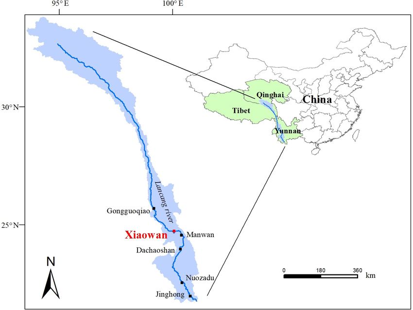
2346                                                      S. Liao et al.: Daily inflow forecasting using ERA-Interim reanalysis

Figure 2. Location of the Xiaowan hydropower station.

                                                                     time series into the input data (Amiri, 2015; Shoaib et al.,
                                                                     2015).

                                                                     3     Methodology

                                                                     3.1    Feature selection via the maximal information
                                                                            coefficient

                                                                     The calculation of the MIC is based on the concept of mu-
                                                                     tual information (MI; Kinney and Atwal, 2014). For a ran-
                                                                     dom variable X, such as observed inflow, the entropy of X is
Figure 3. Daily inflow time series for the Xiaowan hydropower sta-   defined as
tion.                                                                           X
                                                                     H (X) = −      p(x) log p(x),                            (2)
                                                                                 x∈X

                                                                     where p(x) is the probability density function of X = x. Fur-
in the data will be blurred by noise (Zhao et al., 2013). Con-       thermore, for another random variable Y , such as observed
versely, if irrelevant features are chosen, noise will be added      rainfall, the conditional entropy of X given Y may be evalu-
into the model and hinder the learning process. The MIC              ated using the following expression:
is employed to select input data from candidate predictors                          XX
from the reanalysis data set. The lagged inflow and rainfall         H (X|Y ) = −          p(x, y) log p(x|y),                 (3)
                                                                                   x∈X y∈Y
series are identified using the partial autocorrelation func-
tion (PACF) and the cross-correlation function (CCF). The            where H (X|Y ) is the uncertainty of X given knowledge of Y ,
corresponding 95 % confidence interval is used to identify           and p(x, y) and p(x|y) are the joint probability density and
significant correlations. Furthermore, when the correlation          the conditional probability of X = x and Y = y respectively.
coefficient slowly declines and cannot fall into the confidence      The reduction of the original uncertainty of X, due to the
interval, a trial-and-error procedure is used to determine the       knowledge of Y , is called the MI (Amorocho and Espildora,
optimum lag, i.e. starting from one lag and then modifying           1973; Chapman, 1986) and is defined by
the external inputs by successively adding one more lagged

Hydrol. Earth Syst. Sci., 24, 2343–2363, 2020                                      www.hydrol-earth-syst-sci.net/24/2343/2020/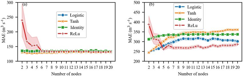
S. Liao et al.: Daily inflow forecasting using ERA-Interim reanalysis                                                                        2347

MI (X, Y ) = H (X) − H (X|Y )
             XX                  p(x, y)
           =        p(x, y) log          .                                 (4)
             x∈Xy∈Y
                                p(x)p(y)

Considering a given data set D, including variable X and Y
with a sample size n, the calculation of the MIC is divided
into three steps. Firstly, scatter plots of X and Y as well
as grids for partitioning, which are called “x-by-y” grids,
are drawn. Let D|G denote the distribution of D divided by
one of the x-by-y grids as G. MI∗ (D, x, y) = max MI(D|G),
where MI(D|G) is the mutual information of D|G. Secondly,
the characteristic matrix is defined as
                 MI∗ (D, x, y)
M(D)x,y =                      .                                           (5)
                log(min(x, y))

Lastly, the MIC is introduced as the maximum value of the
characteristic matrix: MIC(D) = max M(D)x,y , where
                                              xy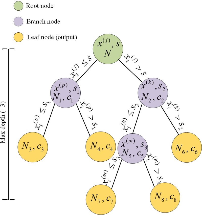
2348                                                           S. Liao et al.: Daily inflow forecasting using ERA-Interim reanalysis

3.2.2    The boosting algorithm                                           and max_depth. Hence, GBRT has six parameters that con-
                                                                          trol model complexity (Fienen et al., 2018), which we ad-
The idea of gradient boosting originated from the observa-                justed for tuning using a trial-and-error procedure.
tion by Breiman (Breiman, 1997) and can be interpreted as an
optimization algorithm based on a suitable cost function. Ex-             3.3   Evaluation criteria of the models
plicit regression gradient-boosting algorithms have been sub-
sequently developed (Friedman, 2001; Mason et al., 1999).                 It is critical to carefully define the meaning of performance
The boosting algorithm used is described in the following.                and to evaluate the performance on the basis of the fore-
Supposing a training data set with n samples (X1 , y1 ), (X2 ,            casting and fitted values of the model compared with his-
y2 ), . . . , (Xn , yn ), a squared loss function is used to train the    torical data. The root-mean-squared error (RMSE) and mean
decision tree:                                                            absolute error (MAE) are the most commonly used criteria
                                                                          to assess model performance, and they are calculated using
                 n
                 X                                                        Eqs. (11) and (12) respectively:
L(y, f (X)) =          (y − f (Xi ))2 .                          (10)                 v
                 i=1                                                                  u n
                                                                                      u1 X                2
                                                                          RMSE = t              Q̂i − Qi                           (11)
The core of the GBRT algorithm is the iterative process of                               n i=1
training the decision with a residual method. The iterative
                                                                                      n
training process of GBRT with M decision trees is explained                        1X
                                                                          MAE =          Q̂i − Qi ,                                 (12)
in the following.                                                                  n i=1
                                           n
  1. Initialization f0 (x) = arg min
                                           P
                                                  L(yi , c);              where Q̂i and Qi are the inflow estimation and observed
                                       c i=1                              value at time i respectively, and n is the number of sam-
                                                                          ples. The RMSE is more sensitive to extremes in the sam-
  2. for m (m = 1, 2, . . . , M) decision trees:
                                                                          ple sets, and it is consequently used to evaluate the model’s
        a. operating i (i = 1, 2, . . . , n) sample points, and us-       ability to simulate flood peaks. The Pearson correlation coef-
           ing the negative gradient of the loss function to              ficient (CORR) is a measure of the strength of the association
           replace the residual    in the current model rmi =             between the observed inflow series and the forecasted inflow
             h            i
           −   ∂L(yi ,f (xi ))
                                              ;                           series, and it is calculated according to Eq. (13):
                 ∂f (xi )      f (x)=fm−1 (x)
                                                                                           Pn

        b. fitting a regression tree with Rmt xi , rmi , the
                                                                                               Qi − Q Q̂i − Q̂
                                                                                           i=1
           ith regression tree with Rmt (t = 1, 2, . . . , T ) as its     CORR = s                     s                 ,          (13)
                                                                                         n           2 P n          2
           corresponding leaf node region is obtained, where                            P
                                                                                             Qi − Q           Q̂i − Q̂
           t is the number of leaf nodes of regression;                               i=1              i=1
        c. for each leaf region t = 1, 2, . . . , T , the
           best fitting   value is calculated by cmt =                    where Q̂ is the mean of the estimation series. The range of
           argmin
                  P
                      L                                                   the CORR is between zero and one and values close to one
              c         (y i , fm−1 (xi ) + c);
                 xi ∈Rmt                                                  demonstrate a perfect estimation result. The Kling–Gupta ef-
        d. the fitting results are updated by adding the fit-             ficiency (KGE) score (Knoben et al., 2019) is also a widely
           ting values obtained to the previous values using              used evaluation index. It can be provided following Eqs. (14)
                                    T
                                    P                                    and (15):
           fmt (xi ) = fm−1 (xi ) +   cmt I xi ∈ Rmt ;                                v
                                                                                      u                                       !2
                                        t=1                                                                      2
                                                                                      u
                                                                                                     2
                                                                                                           σ̂           Q̂
                                                                          KGE = 1 − (CORR − 1) +              −1 +         −1      (14)
                                                                                      t
  3. finally, a strong learning method is obtained fˆ (xi ) =                                              σ            Q
                  M P
                  P   T                                                       v
                                                                               u n
                                                                                                          v
                                                                                                          u n
     fM (xi ) =         cmt I xi ∈ Rmt .                                       u1 X              2       u1 X             2
                  m=1 t=1                                                 σ̂ = t        Q̂i − Q̂ , σ = t             Qi − Q ,      (15)
                                                                                  n i=1                       n i=1
According to the above introduction to GBRT, the parame-
ters of the GBRT can be divided into two categories: boost-               where σ is the standard deviation of the observed values, σ̂ is
ing parameters and tree parameters. The boosting parameters               the standard deviation of the inflow estimation, µ is the mean
include the learning rate and the number of weak learners                 of the observed series and µ̂ is the mean of the inflow esti-
(learning_rate and n_estimators). The learning rate setting is            mation series. The percent bias in the flow duration curve
used to reduce the gradient step. The learning rate influences            high-segment volume (BHV; Yilmaz et al., 2008; Vogel and
the overall time of training: the smaller the value, the more it-         Fennessey, 1994) is presented to estimate the prediction per-
erations are required for training. There are four tree parame-           formance of the model for extreme values. It can be provided
ters: max_leaf_nodes, min_samples_leaf, min_samples_split                 following Eq. (16):

Hydrol. Earth Syst. Sci., 24, 2343–2363, 2020                                          www.hydrol-earth-syst-sci.net/24/2343/2020/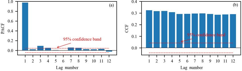
S. Liao et al.: Daily inflow forecasting using ERA-Interim reanalysis                                                                       2349

         H
         P
            Q̂h − Qh
         k=1
BHV =                         × 100,                         (16)
                 H
                 P
                     Qh
               h=1

where h = 1, 2, . . . , H is the inflow index for inflows with
exceedance probabilities lower than 0.02. In this paper, the
inflow threshold of exceedance probabilities equalling 0.02
is 1722 m3 s−1 . The index of agreement (IA; Willmott, 1981)
plays a significant role in evaluating the degree of the agree-
ment between observed series and inflow estimation series.
Similar to CORR, it ranges between zero (no agreement at
all) and one (perfect fit). It is given by
                     n
                     P                2
                           Q̂i − Qi
                     i=1
IA = 1 −   n                              2 .              (17)
           P
                 Q̂i − Q + Qi − Q
           i=1

3.4   Overview of framework

Figure 5 illustrates the overall structure of the framework
presented. This structure consists of two major models:
GBRT and GBRT-MIC. In GBRT, we measure the relevance
of the different lags in observed inflow and rainfall with ob-
served inflow at the time of forecast using the partial auto-
correlation function (PACF) and the cross-correlation func-          Figure 5. Overview of the framework.
tion (CCF; Badrzadeh et al., 2013), and we select appropri-
ate lags as predictors for the model using hypothesis testing
                                                                     et al., 2012). Thus, the static multistep forecasting strategy
and trial-and-error procedures. Data preprocessing and fea-
                                                                     is employed in this paper. As the static strategy does not use
ture scaling are then carried out for selected predictors. Next,
                                                                     any approximated values to compute the forecasts, it is not
the data set is divided into a training set, a validation set, and
                                                                     prone to the accumulation of errors. The model structures of
a testing set according to the length of each data set, which is
                                                                     GBRT and GBRT-MIC are as follows:
specified in advance (in Sect. 2.2). A grid search algorithm,
which is an exhaustive search-all candidate parameter combi-         Q̂It+T = f θ It ; Qt , Qt−1 , . . ., Qt+1−p , Rt , Rt−1 , . . .,
nation method, is guided to the optimization model parame-
                                                                            Rt+1−q (T = 1, 2, . . ., 10)                                    (18)
ters by the evaluation of the validation set for each lead time
(Chicco, 2017). Lastly, the prediction results are evaluated         Q̂II
                                                                       t+T   =f    θ II
                                                                                     t ; Qt , Qt−1 ,   . . ., Qt+1−p , Rt , Rt−1 , . . .,
based on the testing set. Compared with GBRT, GBRT-MIC
                                                                             Rt+1−q , Et1 , Et2 , . . ., Etk (T = 1, 2, . . ., 10),         (19)
adds reanalysis data which are selected via MIC (in Sect. 3.1)
as the model input. Moreover, GBRT-MIC also calculates the
                                                                     where Q̂It+T and Q̂II t+T are the forecasted values of GBRT
importance of features according to the prediction results and
                                                                     and GBRT-MIC at lead time T of current time t respectively;
ranks the features (Louppe, 2014).
                                                                     θ It and θ II
                                                                                t are parameters of GBRT and GBRT-MIC at lead
   It is difficult to perform multistep forecasting due to the ac-
                                                                     time T of current time t respectively; p and q are lags of the
cumulation of errors, reduced accuracy and increased uncer-
                                                                     observed inflow and rainfall determined using the PACF and
tainty. Therefore, the current state of multistep-ahead fore-
                                                                     CCF respectively; Et represents the features from reanalysis
casting is reviewed. There are two main strategies that one
                                                                     data at the current time t; and k is the number of features
can use for multistep forecasting for single output, namely,
                                                                     from the reanalysis data determined via the MIC.
static (direct) multistep forecasting and recursive multistep
forecasting (Bontempi et al., 2012; Taieb et al., 2012). The
recursive forecasting strategy is biased when the underlying         4   Experimental results and discussion
model is nonlinear, and it is sensitive to the estimation error
as estimated values, instead of actual values, are used more         In order to compare them with GBRT-MIC, the ANN-MIC,
often as the forecasts move further into the future (Bontempi        SVR-MIC and MLR-MIC models, which were obtained by

www.hydrol-earth-syst-sci.net/24/2343/2020/                                         Hydrol. Earth Syst. Sci., 24, 2343–2363, 2020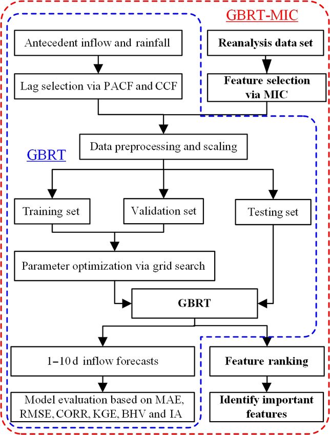
2350                                                       S. Liao et al.: Daily inflow forecasting using ERA-Interim reanalysis

Figure 6. (a) The PACF plot of Xiaowan daily inflow, and (b) the CCF of Xiaowan rainfall and inflow.

Table 1. The candidate inputs via the PACF and CCF.

                  No.    Input
                  1      Qt−1 , Qt−4
                  2      Qt−1 , Qt−4 , Rt−1
                  3      Qt−1 , Qt−4 , Rt−1 , Rt−2
                  4      Qt−1 , Qt−4 , Rt−1 , Rt−2 , Rt−3
                  5      Qt−1 , Qt−4 , Rt−1 , Rt−2 , Rt−3 , Rt−4
                  6      Qt−1 , Qt−4 , Rt−1 , Rt−2 , Rt−3 , Rt−4 , Rt−5
                  7      Qt−1 , Qt−4 , Rt−1 , Rt−2 , Rt−3 , Rt−4 , Rt−5 , Rt−6
                  8      Qt−1 , Qt−4 , Rt−1 , Rt−2 , Rt−3 , Rt−4 , Rt−5 , Rt−6 , Rt−7
                  9      Qt−1 , Qt−4 , Rt−1 , Rt−2 , Rt−3 , Rt−4 , Rt−5 , Rt−6 , Rt−7 , Rt−8
                  10     Qt−1 , Qt−4 , Rt−1 , Rt−2 , Rt−3 , Rt−4 , Rt−5 , Rt−6 , Rt−7 , Rt−8 , Rt−9
                  11     Qt−1 , Qt−4 , Rt−1 , Rt−2 , Rt−3 , Rt−4 , Rt−5 , Rt−6 , Rt−7 , Rt−8 , Rt−9 , Rt−10
                  12     Qt−1 , Qt−4 , Rt−1 , Rt−2 , Rt−3 , Rt−4 , Rt−5 , Rt−6 , Rt−7 , Rt−8 , Rt−9 , Rt−10 , Rt−11
                  13     Qt−1 , Qt−4 , Rt−1 , Rt−2 , Rt−3 , Rt−4 , Rt−5 , Rt−6 , Rt−7 , Rt−8 , Rt−9 , Rt−10 , Rt−11 , Rt−12

replacing GBRT in the framework with ANN, SVR and MLR                    the lagged rainfall series. A total of 13 input structures are
respectively, are also employed for inflow forecasting with              tried (Table 1), and the trial results are shown in Fig. A1.
lead times of 1–10 d. As mentioned previously, six indices,              The results indicate that 7th input structure shows the best
the MAE, RMSE, CORR, KGE, BHV and IA, are calcu-                         performance. Accordingly, rainfall series from 1 to 6 d lag
lated to evaluate the performance of models based on the                 are selected as the model input. As mentioned previously,
testing set. We also explored the feature importance based               based on the MIC between inflow and the reanalysis variable
on the GBRT-MIC model (Louppe, 2014). All computations                   (Table A1), a trial-and-error procedure is used to determine
carried out in this paper were performed on a ThinkPad P1                the optimal input subset. A total of 26 input structures are
workstation containing an Intel Core i7-9850H CPU with                   tried (Table 2), and the trial results are shown in Fig. A2. The
2.60 GHz and 16.0 GB of RAM, using the version 3.7.10 of                 results show that 8th input structure shows the best perfor-
Python (Python Software Foundation, 2020), which is pow-                 mance; thus, the predictors nos. 1–8 in Table A1 are selected
erful, fast and open, and the scikit-learn package (Pedregosa            as the model input. Finally, a total of 16 variables including
et al., 2011).                                                           8 observed variables and 8 reanalysis variables are selected
                                                                         as the model input (Table 3). As shown in Table 3, nos. 9–
4.1    Feature selection                                                 18 are reanalysis variables, and the range of the MIC of the
                                                                         reanalysis variables selected is 0.643 to 0.847. Furthermore,
                                                                         no. 9 and nos. 13–16 are variables related to temperature.
Figure 6 shows the PACF, CCF and the corresponding 95 %
                                                                         Soil temperature level 3 (no. 9) is the temperature of the soil
confidence interval from lag 1 to lag 12. The PACF shows
                                                                         in layer 3 (28–100 cm, where the surface is at 0 cm). The
significant autocorrelation at lag 1 and lag 4 respectively
                                                                         temperature of the snow layer (no. 13) gives the tempera-
(Fig. 6a); thus, inflow series 1 and 4 d lag are selected as the
                                                                         ture of the snow layer from the ground to the snow–air inter-
model inputs. The CCF between inflow and rainfall gradu-
                                                                         face. Nos. 10–12 are variables related to the water content of
ally decreases as the time lag increases (Fig. 6b) and cannot
                                                                         the atmosphere. The 2 m dewpoint temperature (no. 10) is a
fall into the 95 % confidence interval. Therefore, a trial-and-
                                                                         measure of the humidity of the air, and, when combined with
error procedure is used to determine the optimal selection of

Hydrol. Earth Syst. Sci., 24, 2343–2363, 2020                                           www.hydrol-earth-syst-sci.net/24/2343/2020/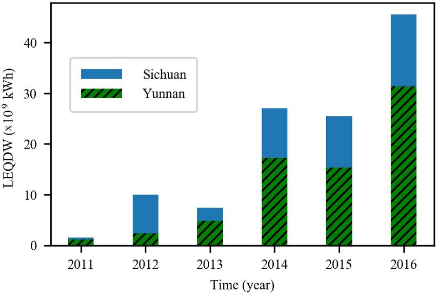
S. Liao et al.: Daily inflow forecasting using ERA-Interim reanalysis                                                                                                         2351

Table 2. The candidate inputs from reanalysis data via the MIC.

     No.      Input
     1        obs, stl3t−1
     2        obs,stl3t−1 , d2mt−1
     3        obs,stl3t−1 , d2mt−1 , tcwvt−1
     4        obs,stl3t−1 , d2mt−1 , tcwvt−1 , tcwt−1
     5        obs,stl3t−1 , d2mt−1 , tcwvt−1 , tcwt−1 , stl2t−1
     6        obs,stl3t−1 , d2mt−1 , tcwvt−1 , tcwt−1 , stl2t−1 , mn2tt−1
     7        obs,stl3t−1 , d2mt−1 , tcwvt−1 , tcwt−1 , stl2t−1 , mn2tt−1 , tsnt−1
     8        obs,stl3t−1 , d2mt−1 , tcwvt−1 , tcwt−1 , stl2t−1 , mn2tt−1 , tsnt−1 , stl4t−1
     9        obs,stl3t−1 , d2mt−1 , tcwvt−1 , tcwt−1 , stl2t−1 , mn2tt−1 , tsnt−1 , stl4t−1 , stl1t−1
     10       obs,stl3t−1 , d2mt−1 , tcwvt−1 , tcwt−1 , stl2t−1 , mn2tt−1 , tsnt−1 , stl4t−1 , stl1t−1 , rot−1
     11       obs,stl3t−1 , d2mt−1 , tcwvt−1 , tcwt−1 , stl2t−1 , mn2tt−1 , tsnt−1 , stl4t−1 , stl1t−1 , rot−1 , swvl1t−1
     12       obs,stl3t−1 , d2mt−1 , tcwvt−1 , tcwt−1 , stl2t−1 , mn2tt−1 , tsnt−1 , stl4t−1 , stl1t−1 , rot−1 , swvl1t−1 , swvl2t−1
     13       obs,stl3t−1 , d2mt−1 , tcwvt−1 , tcwt−1 , stl2t−1 , mn2tt−1 , tsnt−1 , stl4t−1 , stl1t−1 , rot−1 , swvl1t−1 , swvl2t−1 , swvl3t−1
     14       obs, rea, t2mt−1
     15       obs, rea, t2mt−1 , swvl4t−1
     16       obs, rea, t2mt−1 , swvl4t−1 , mx2tt−1
     17       obs, rea, t2mt−1 , swvl4t−1 , mx2tt−1 , sft−1
     18       obs, rea, t2mt−1 , swvl4t−1 , mx2tt−1 , sft−1 , cpt−1
     19       obs, rea, t2mt−1 , swvl4t−1 , mx2tt−1 , sft−1 , cpt−1 , tpt−1
     20       obs, rea, t2mt−1 , swvl4t−1 , mx2tt−1 , sft−1 , cpt−1 , tpt−1 , rsnt−1
     21       obs, rea, t2mt−1 , swvl4t−1 , mx2tt−1 , sft−1 , cpt−1 , tpt−1 , rsnt−1 , lspt−1
     22       obs, rea, t2mt−1 , swvl4t−1 , mx2tt−1 , sft−1 , cpt−1 , tpt−1 , rsnt−1 , lspt−1 , sdt−1
     23       obs, rea, t2mt−1 , swvl4t−1 , mx2tt−1 , sft−1 , cpt−1 , tpt−1 , rsnt−1 , lspt−1 , sdt−1 , smltt−1
     24       obs, rea, t2mt−1 , swvl4t−1 , mx2tt−1 , sft−1 , cpt−1 , tpt−1 , rsnt−1 , lspt−1 , sdt−1 , smltt−1 , istl1t−1
     25       obs, rea, t2mt−1 , swvl4t−1 , mx2tt−1 , sft−1 , cpt−1 , tpt−1 , rsnt−1 , lspt−1 , sdt−1 , smltt−1 , istl1t−1 , istl3t−1
     26       obs, rea, t2mt−1 , swvl4t−1 , mx2tt−1 , sft−1 , cpt−1 , tpt−1 , rsnt−1 , lspt−1 , sdt−1 , smltt−1 , istl1t−1 , istl3t−1 , istl2t−1
   Note: “obs” represents the selected observed optimal input set, obs = {Qt−1 , Qt−4 , Rt−1 , Rt−2 , Rt−3 , Rt−4 , Rt−5 , Rt−6 }. “rea” represents the selected input set from
   the reanalysis, rea = {stl3t−1 , d2mt−1 , tcwvt−1 , tcwt−1 , stl2t−1 , mn2tt−1 , tsnt−1 , stl4t−1 , stl1t−1 , rot−1 , swvl1t−1 , swvl2t−1 , swvl3t−1 }.

Table 3. List of input data for GBRT-MIC. There are of two input types, observed and reanalysis variables. The reanalysis variables are
available twice a day at 00:00 and 12:00 UTC. The cumulative variables (e.g. total column water) are the sum of two periods, and the
instantaneous variables (e.g. 2 m dewpoint temperature) are the mean of two periods.

                                    No.      Description                                Index           Unit             MIC         Type
                                    1        Inflow on day t − 1                        Qt−1            (m3 s−1 )          –         Obs.
                                    2        Inflow on day t − 2                        Qt−2            (m3 s−1 )          –         Obs.
                                    3        Rainfall on day t − 1                      Rt−1            (mm)               –         Obs.
                                    4        Rainfall on day t − 2                      Rt−2            (mm)               –         Obs.
                                    5        Rainfall on day t − 3                      Rt−3            (mm)               –         Obs.
                                    6        Rainfall on day t − 4                      Rt−4            (mm)               –         Obs.
                                    7        Rainfall on day t − 5                      Rt−5            (mm)               –         Obs.
                                    8        Rainfall on day t − 6                      Rt−6            (mm)               –         Obs.
                                    9        Soil temperature level 3                   stl3t−1         (K)              0.847       ERA-I.
                                    10       2 m dewpoint temperature                   d2mt−1          (K)              0.781       ERA-I.
                                    11       Total column water vapour                  tcwvt−1         (kg m−2 )        0.699       ERA-I.
                                    12       Total column water                         tcwt−1          (kg m−2 )        0.699       ERA-I.
                                    13       Soil temperature level 2                   stl2t−1         (K)              0.689       ERA-I.
                                    14       Minimum temperature at 2 m                 mn2tt−1         (K)              0.684       ERA-I.
                                    15       Temperature of snow layer                  tsnt−1          (K)              0.664       ERA-I.
                                    16       Soil temperature level 4                   stl4t−1         (K)              0.643       ERA-I.

www.hydrol-earth-syst-sci.net/24/2343/2020/                                                                    Hydrol. Earth Syst. Sci., 24, 2343–2363, 2020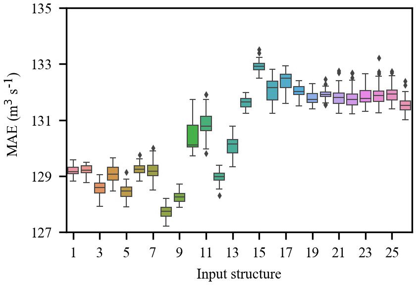
2352                                                    S. Liao et al.: Daily inflow forecasting using ERA-Interim reanalysis

Figure 7. Sensitivity of the activation function and the number of nodes in the hidden layer to the MAE of the ANN-MIC model: (a) 1 d
ahead and (b) 10 d ahead. The shaded area represents the 95 % confidence interval obtained by a bootstrap of 50 trials.

Table 4. Four commonly used activation functions for ANN-MIC.        tion function and the number of nodes of the hidden layer are
                                                                     determined by selecting the minimal MAE of the validation
                Name       Functional expression                     set for each lead time. The results of the trials show that tanh
                                                                     and the logistic function are the two more robust activation
                Logistic   f (x) = 1+e1 −x
                                     x    −x                         functions (Fig. 7), and ANN, with fewer nodes, is inclined to
                Tanh       f (x) = eex −e
                                       +e−x                          obtain a lower error. The optimal parameter combination for
                Identity   f (x) = x                                 each lead time is listed in Table 5. It can be seen that the op-
                ReLU       f (x) = max(0, x)                         timal number of nodes is 2, 3 or 4, and the optimal activation
                                                                     function is either tanh or the logistic function.
                                                                        For SVR, according to Lin et al. (2006) and Dibike et al.
temperature and pressure, it can be used to calculate the rel-       (2001), the radial basis function (RBF) outperforms other
ative humidity. The total column water vapour (no. 11) is the        kernel functions for runoff modelling; thus, RBF is used as
total amount of water vapour, which is a fraction of the total       the kernel function in this study. There are three parameters
column water. The total column water (no. 12) is the sum of          that need to be adjusted. Firstly, an appropriate tuning range
the water vapour, liquid water, cloud ice, rain and snow in a        of each parameter is determined by a trial-and-error proce-
column extending from the surface of the Earth to the top of         dure. Then, to reach at an optimal choice of these parame-
the atmosphere. The volumetric soil water layer 1 (no. 19) is        ters, the MAE is used to optimize the parameters using grid
the volume of water in soil layer 1. In summary, all the se-         search. The optimal tuning parameters of SVR are shown in
lected predictors are interpretable and have a good physical         Table 5. As mentioned earlier, for GBRT, there are six param-
connection to inflow.                                                eters need to be adjusted. In order to obtain an optimal pa-
                                                                     rameter combination as soon as possible, we optimize all pa-
4.2    Hyperparameter optimization                                   rameters in two steps. Firstly, n_estimators and learning_rate
                                                                     are fixed to 100 and 0.1 respectively. The max_leaf_nodes,
For machine-learning methods, hyperparameters are param-             min_samples_leaf, max_depth and min_samples_split tun-
eters that are set before training and cannot be directly learnt     ing parameters generate 40 000 models at each lead time.
from the regular training process. In order to improve the           Secondly, after the tree parameters are determined, learn-
performance of models, it is imperative to tune the hyper-           ing_rate is modified to 0.01 and n_estimators is determined
parameters of models. The grid search function is employed           using grid search. To accommodate the computational bur-
to tune the hyperparameters of GBRT, GBRT-MIC, ANN-                  den, all models are distributed among about 12 central pro-
MIC and SVR-MIC. After a review of the available literature          cessing units (CPUs), and the total wall time for the runs is
(Badrzadeh et al., 2013; Rasouli et al., 2012), an optimizer         about 7 h for GBRT_MIC and GBRT. Table 6 lists the opti-
in the family of quasi-Newton methods, namely L-BFGS, is             mal tuning parameters for GBRT and GBRT-MIC.
chosen as the training algorithm for the ANN, and the num-
ber of hidden layers is fixed to three. Another two parame-          4.3   Input comparison
ters, namely the activation function and the number of nodes
of the hidden layer, need to be adjusted. A range of 2–20 neu-       Figure 8 illustrates the performance indices of GBRT and
rons and four commonly used activation functions (Table 4)           GBRT-MIC for the testing set (1 January 2017–31 Decem-
are selected by grid search. To alleviate the influence of the       ber 2018) at lead times of 1–10 d. It is obvious that the re-
random initialization of weights, 50 ANN-MIC models are              analysis data selected by the MIC greatly improves upon the
trained for each parameter combination. The optimal activa-          GBRT forecasting at both short and long lead times. In par-

Hydrol. Earth Syst. Sci., 24, 2343–2363, 2020                                      www.hydrol-earth-syst-sci.net/24/2343/2020/
S. Liao et al.: Daily inflow forecasting using ERA-Interim reanalysis 2353
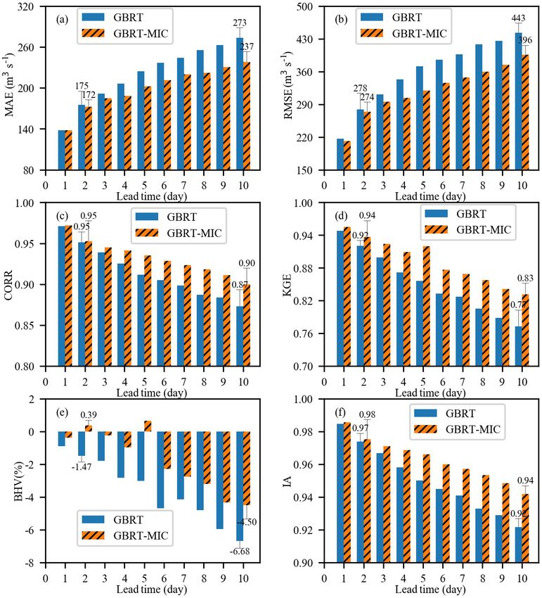
Figure 8. Performance of GBRT and GBRT-MIC for the testing set (2017–2018) in terms of the following six indices: (a) MAE, (b) RMSE,
(c) CORR, (d) KGE, (e) BHV and (f) IA.
Table 5. Tuning parameters for ANN-MIC and SVR-MIC.
Model Tuning Tuning range 1 2 3 4 5 6 7 8 9 10
parameter
ANN-MIC Structure – 19–4–1 19–2–1 19–3–1 19–2–1 19–2–1 19–2–1 19–2–1 19–2–1 19–2–1 19–2–1
Activation – Tanh Tanh Logistic Logistic Logistic Logistic Logistic Logistic Tanh Tanh
function
SVR-MIC C (1, 100, 20) 6.2105 1.0000 1.0000 1.0000 11.4211 1.0000 1.0000 6.2105 1.0000 6.2105
(0.001, 0.1, 20) 0.0069 0.0084 0.0017 0.0079 0.0017 0.0001 0.0022 0.0006 0.0048 0.0043
γ (0.001, 0.1, 20) 0.0323 0.0583 0.0844 0.0271 0.0062 0.0218 0.0375 0.0166 0.0687 0.0166
h i
Note: the bold text, (min, max, step) represents min + max−min max−min max−min
step−1 × 0, min + step−1 × 1, . . ., min + step−1 × (step − 1) .
www.hydrol-earth-syst-sci.net/24/2343/2020/ Hydrol. Earth Syst. Sci., 24, 2343–2363, 20202354 S. Liao et al.: Daily inflow forecasting using ERA-Interim reanalysis
Table 6. Tuning parameters for GBRT and GBRT-MIC.
Tuning parameter Tuning range Optimal parameters (lead times of 1–10 d)
GBRT GBRT-MIC
max_leaf_nodes [2, 4, 6, . . . , 40] 8, 4, 4, 4, 4, 2, 4, 2, 2, 2 7, 9, 13, 7, 15, 4, 5, 4, 4, 17
min_samples_leaf [1, 6, 11, . . . , 46] 6, 31, 1, 1, 1, 31, 6, 1, 6, 1 2, 7, 2, 4, 2, 1, 10, 10, 8, 1
max_depth [1, 2, 3, . . . , 10] 3, 2, 2, 2, 3, 1, 3, 1, 1, 1 4, 6, 8, 5, 9, 9, 2, 2, 7, 2
min_samples_split [2, 4, 6, . . . , 40] 18, 2, 16, 16, 24, 2, 16, 2, 2, 2 18, 15, 12, 13, 8, 3, 19, 3, 19, 8
n_estimators [100, 200, 300, . . . , 4000] 1100, 900, 1200, 700, 700, 3800, 2700, 1300, 900, 1000,
1200, 600, 1100, 900, 900 700, 1400, 2000, 1300, 1200
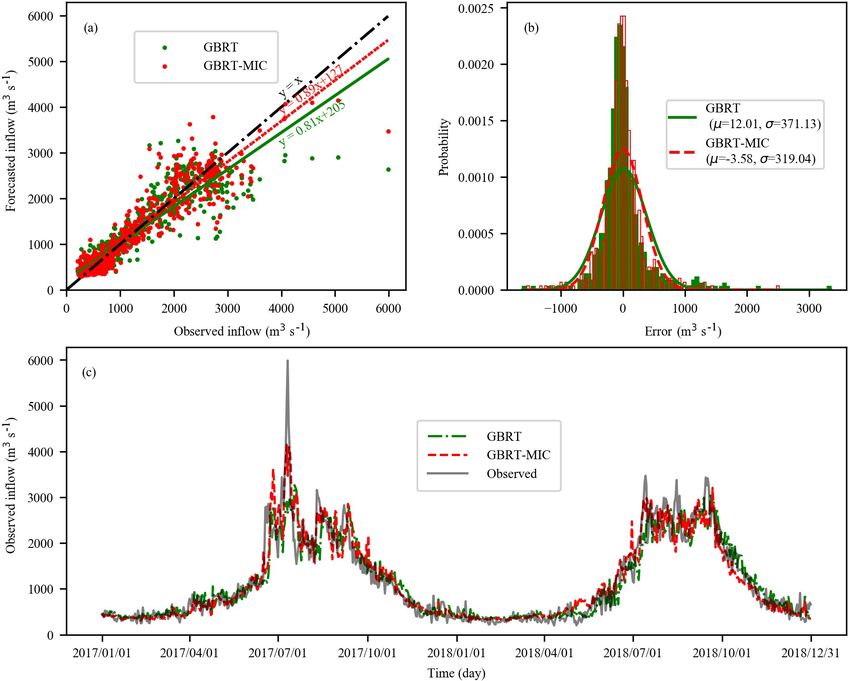
Figure 9. The 5 d ahead inflow forecasts of GBRT and GBRT-MIC for the testing set (2017–2018, 730 d). (a) Observed versus forecasted
inflow. (b) The histogram of the prediction error of the testing set. (c) Comparison of the observed and forecasted inflow.
ticular, for the longer lead times, GBRT-MIC significantly the CORR, KGE and IA of GBRT-MIC increase by 0.2 %,
outperforms GBRT. From Fig. 8a, it can be noted that the 2.2 %, 1.0 % for 2 d ahead forecasting and 3.4 %, 7.8 % and
MAE of GBRT-MIC decreases from 175 to 172, which is 2.2 % for 10 d ahead forecasting respectively. Figure 8e com-
a decrease of 1.74 %, for 2 d ahead forecasting, and it de- pares the BHV values for GBRT and GBRT-MIC and indi-
creases from 273 to 237, which is a decrease of 13.18 %, for cates that the reanalysis data can enhance the forecasting of
10 d ahead forecasting compared with GBRT. From Fig. 8b, extreme values. Figure 9a shows the 5 d ahead forecasted in-
it can be seen that the RMSE of GBRT-MIC achieves a 1.4 % flow of GBRT-MIC and GBRT versus the observed inflow
and 10.6 % reduction for 2 and 10 d ahead forecasting respec- in the testing set. The slopes of the fitting curves of GBRT-
tively compared with GBRT. Figure 8c, d and f show that MIC and GBRT are 0.89 and 0.81 respectively; this also
Hydrol. Earth Syst. Sci., 24, 2343–2363, 2020 www.hydrol-earth-syst-sci.net/24/2343/2020/S. Liao et al.: Daily inflow forecasting using ERA-Interim reanalysis 2355
Table 7. Performance indices of the training set.
Index Model 1 2 3 4 5 6 7 8 9 10
MAE (m3 s−1 ) GBRT-MIC 56 63 78 122 89 163 161 155 161 172
SVR-MIC 98 126 144 162 173 183 188 194 197 203
ANN-MIC 99 129 148 162 172 184 192 196 203 205
MLR-MIC 103 136 159 175 187 198 207 215 221 228
RMSE (m3 s−1 ) GBRT-MIC 77 87 107 185 124 257 255 245 254 278
SVR-MIC 153 212 247 280 300 319 329 337 344 353
ANN-MIC 151 206 240 264 284 304 318 328 334 339
MLR-MIC 157 214 250 275 295 315 330 342 352 361
CORR GBRT-MIC 0.9952 0.9940 0.9908 0.9724 0.9877 0.9464 0.9468 0.9510 0.9476 0.9366
SVR-MIC 0.9811 0.9641 0.9511 0.9380 0.9286 0.9186 0.9126 0.9073 0.9039 0.8977
ANN-MIC 0.9815 0.9653 0.9528 0.9424 0.9331 0.9232 0.9156 0.9101 0.9066 0.9036
MLR-MIC 0.9801 0.9628 0.9485 0.9376 0.9278 0.9172 0.9090 0.9019 0.8959 0.8900
KGE GBRT-MIC 0.9884 0.9827 0.9738 0.9439 0.9642 0.9009 0.9069 0.9099 0.9002 0.8877
SVR-MIC 0.9618 0.9207 0.8982 0.8613 0.8445 0.8266 0.8223 0.8247 0.8149 0.8103
ANN-MIC 0.9735 0.9508 0.9325 0.9177 0.9048 0.8907 0.8800 0.8724 0.8668 0.8611
MLR-MIC 0.9718 0.9473 0.9272 0.9117 0.8979 0.8829 0.8713 0.8613 0.8528 0.8444
BHV (%) GBRT-MIC −0.3025 −0.6382 −0.8986 −1.3422 −1.4019 −1.5485 −1.7486 −1.7692 −2.6647 −3.0375
SVR-MIC −1.3488 −3.3959 −4.0686 −6.9058 −7.5421 −8.2216 −6.9950 −6.1996 −6.2406 −5.6687
ANN-MIC −0.1814 −0.2586 −0.7710 −0.7723 −0.6249 −0.6815 −0.6878 −0.8821 −0.6487 −0.1239
MLR-MIC −0.4668 −1.0527 −1.5863 −1.9709 −1.9477 −2.1634 −2.0182 −1.8074 −2.0454 −1.7473
IA GBRT-MIC 0.9976 0.9969 0.9952 0.9854 0.9935 0.9706 0.9712 0.9734 0.9712 0.9650
SVR-MIC 0.9902 0.9804 0.9727 0.9636 0.9574 0.9506 0.9472 0.9449 0.9421 0.9386
ANN-MIC 0.9906 0.9820 0.9752 0.9695 0.9643 0.9586 0.9541 0.9509 0.9487 0.9468
MLR-MIC 0.9898 0.9807 0.9729 0.9668 0.9613 0.9551 0.9502 0.9460 0.9423 0.9387
Note: the bold text represents the values of the performance criterion for the best fitted models.
demonstrates that GBRT-MIC can obtain more accurate in- cient in the training set than other models at lead times of
flow forecasting than GBRT. Figure 9b illustrates the dis- 1–10 d, which demonstrates that GBRT-MIC has a power-
tribution of the forecast errors of GBRT and GBRT-MIC. ful fitting ability. Meanwhile, all machine-learning models
The results show that the prediction error of two models has obtain better forecasted results than MLR-MIC, which can-
an approximately normal distribution. This demonstrates that not capture nonlinear relationships. It should be noted that
the prediction error contains information that is not extracted ANN-MIC has the best performance for extreme values in
by the model and that more errors of the forecasted inflow terms of the BHV in the training set. As shown in Table 8,
concentrate at around zero for GBRT-MIC than for GBRT. GBRT-MIC performs best for the testing set at lead times of
Figure 9c provides forecasted inflow time series (from the 4–10 d in terms of the above-mentioned six indices. At a lead
testing set) for GBRT-MIC and GBRT at a lead time of 5 d. It time of 10 d, the KGE of GBRT-MIC even reached 0.8317.
can be seen that GBRT-MIC shows great performance com- At lead times of 1–3 d, three machine-learning models obtain
pared with GBRT, especially for extreme values. This re- good performance and outperform MLR-MIC. The machine-
veals that the problem of inaccurate extreme value predic- learning models can acquire enough information to perform
tion that has arisen in areas with concentrated rainfall for the forecasting at short lead times (1–3 d). The performance in-
GBRT model could be mitigated by incorporating the reanal- dices of these four models in the testing set (2017–2018) at
ysis data identified by the MIC. lead times of 1–10 d are presented in Fig. 10. The results in-
dicate that the performance of these four models decreases
4.4 Model comparison (higher MAE, RMSE and BHV, and lower CORR, KGE
and IA) as the lead time increases. As mentioned earlier, the
GBRT-MIC, SVR-MIC and ANN-MIC with the optimal four models perform equally well for 1 to 3 d ahead forecast-
model parameters are employed for inflow forecasting of 1 ing, whereas significant differences among their performance
to 10 d ahead. The summarized results for the training and are found as lead times exceed 3 d. This clearly indicates
testing set are presented in Tables 7 and 8 respectively. To that GBRT produces much higher CORR, KGE and IA val-
avoid the problem of local minima, 50 ANN-MIC models ues and lower MAE, RMSE and BHV values than the other
are trained for each lead time, and the median of the predic- three models for 4–10 d ahead forecasting, although ANN-
tions of the 50 models is used as the final prediction. It is MIC performs almost as well as GBRT-MIC for 10 d ahead
clear from Table 7 that the GBRT-MIC model is more effi- forecasting. It should be noted that SVR shows the worst
www.hydrol-earth-syst-sci.net/24/2343/2020/ Hydrol. Earth Syst. Sci., 24, 2343–2363, 20202356 S. Liao et al.: Daily inflow forecasting using ERA-Interim reanalysis
Figure 10. Performance of GBRT-MIC, SVR-MIC, ANN-MIC and MLR-MIC for the testing set (2017–2018) in term of the following six
indices: (a) MAE, (b) RMSE, (c) CORR, (d) KGE, (e) BHV and (f) IA.
performance according to the BHV and KGE values, and (e.g. stl3t−10 and d2mt−10 ) from the reanalysis data have
this demonstrates that SVR cannot capture extreme values. a high relative importance at longer lead times (Fig. 11b).
On the contrary, GBRT-MIC significantly outperforms other Based on the analysis of the concepts of stl3t−10 and tcwt−10
models in terms of the BHV at lead times of 1–10 d, which (Sect. 4.1), we infer that the temperature near the ground im-
indicates that GBRT-MIC is the most successful model with pacts the inflow by affecting the melting of snow, which is
respect to obtaining extreme values among all of the models consistent with the fact that the Lancang River is a snowmelt
developed in this paper. river. The 10 d lag observed time series (Qt−10 ) is also very
important, which indicates the long memory of inflow se-
4.5 Feature importance ries (Salas, 1993). Meanwhile, it is found that the reanalysis
data provide important information for inflow forecasting at
A benefit of using gradient boosting is that after the boosted longer lead times.
trees are constructed, the relative importance scores for each
feature can be acquired to estimate the contribution of each
feature to inflow forecasting. Figure 11 shows the feature 5 Conclusions
importance based on GBRT-MIC for lead times of 1 and
10 d respectively. The 1 d lag observed time series (Qt−1 ) In this study, GBRT-MIC is employed to make inflow fore-
is more important for shorter lead times (Fig. 11a), which casts for lead times of 1–10 d, and ANN-MIC, SVR-MIC
demonstrates that the historical observed values are essen- and MLR-MIC are developed to compare with GBRT-MIC.
tial to inflow forecasting at shorter lead times. The features The reanalysis data selected by the MIC and the antecedent
Hydrol. Earth Syst. Sci., 24, 2343–2363, 2020 www.hydrol-earth-syst-sci.net/24/2343/2020/S. Liao et al.: Daily inflow forecasting using ERA-Interim reanalysis 2357
Table 8. Performance indices of the testing set.
Index Model 1 2 3 4 5 6 7 8 9 10
MAE (m3 s−1 ) GBRT-MIC 137 172 185 188 202 211 219 222 230 237
SVR-MIC 131 164 182 197 212 223 227 231 233 237
ANN-MIC 132 163 182 198 211 221 225 230 239 238
MLR-MIC 138 173 195 213 230 244 248 252 259 263
RMSE (m3 s−1 ) GBRT-MIC 211 274 295 304 319 336 347 359 374 396
SVR-MIC 200 263 303 342 366 387 395 403 407 413
ANN-MIC 199 258 296 324 341 362 376 391 402 399
MLR-MIC 205 268 314 347 369 391 404 413 423 429
CORR GBRT-MIC 0.9722 0.9526 0.9449 0.9414 0.9354 0.9285 0.9236 0.9181 0.9112 0.8997
SVR-MIC 0.9751 0.9575 0.9434 0.9300 0.9196 0.9099 0.9058 0.8999 0.8993 0.8950
ANN-MIC 0.9752 0.9580 0.9444 0.9333 0.9257 0.9163 0.9091 0.9017 0.8956 0.8975
MLR-MIC 0.9738 0.9545 0.9374 0.9231 0.9126 0.9012 0.8940 0.8893 0.8834 0.8802
KGE GBRT-MIC 0.9550 0.9367 0.9244 0.9092 0.9200 0.8769 0.8693 0.8580 0.8417 0.8317
SVR-MIC 0.9520 0.9055 0.8797 0.8347 0.8158 0.7950 0.7915 0.7941 0.7822 0.7786
ANN-MIC 0.9625 0.9352 0.9115 0.8953 0.8808 0.8658 0.8530 0.8440 0.8371 0.8313
MLR-MIC 0.9605 0.9284 0.9011 0.8800 0.8620 0.8452 0.8319 0.8232 0.8137 0.8054
BHV (%) GBRT-MIC −0.3826 0.3880 −0.2319 −0.9629 0.6566 −2.2766 −2.7422 −3.1924 −4.3363 −4.5040
SVR-MIC −1.3382 −4.0253 −5.3037 −8.2410 −9.4167 −10.0357 −9.6049 −8.9452 −9.6886 −10.1058
ANN-MIC −0.1228 −0.9608 −1.8150 −2.0839 −2.7642 −3.3509 −4.4831 −4.7424 −5.1999 −5.5886
MLR-MIC −0.8093 −2.3244 −3.4945 −4.4210 −4.8268 −5.5955 −6.5914 −6.6302 −6.8944 −7.3080
IA GBRT-MIC 0.9856 0.9753 0.9710 0.9686 0.9661 0.9601 0.9571 0.9535 0.9485 0.9419
SVR-MIC 0.9869 0.9763 0.9676 0.9568 0.9495 0.9421 0.9396 0.9372 0.9351 0.9326
ANN-MIC 0.9872 0.9779 0.9701 0.9637 0.9590 0.9532 0.9486 0.9442 0.9405 0.9408
MLR-MIC 0.9865 0.9759 0.9661 0.9577 0.9511 0.9441 0.9392 0.9360 0.9320 0.9295
Note: the bold text represents the values of the performance criterion for the best fitted models.
Figure 11. Feature importance obtained by GBRT-MIC: (a) 1 d ahead and (b) 10 d ahead.
inflow and the rainfall records selected by the PACF and ues. According to a comparison of the forecasted results of
CCF are used as predictors to drive the models. These mod- GBRT and GBRT-MIC, we conclude that GBRT-MIC can
els are compared using six evaluation criteria: the MAE, be used for more accurate and reliable inflow forecasting
RMSE, CORR, KGE, BHV and IA. It is shown that GBRT- at lead times of 1–10 d and that reanalysis data selected by
MIC, ANN-MIC and SVR-MIC outperform MLR-MIC at the MIC greatly improve upon the GBRT forecasting, espe-
lead times of 1–10 d, and GBRT-MIC performs best at lead cially for lead times of 4–10 d. In addition, the feature im-
times of 4–10 d, especially for the forecasting of extreme val- portance achieved by GBRT-MIC demonstrates that soil tem-
www.hydrol-earth-syst-sci.net/24/2343/2020/ Hydrol. Earth Syst. Sci., 24, 2343–2363, 20202358 S. Liao et al.: Daily inflow forecasting using ERA-Interim reanalysis perature, the total amount of water vapour in a column and dewpoint temperature near the ground contribute to increas- ing the prediction accuracy of inflow at longer lead times. In summary, the framework developed integrates GBRT and reanalysis data selected by the MIC and can perform inflow forecasting well at lead times of 1–10 d. The results of this study are of significance as they can assist power stations in making power generation plans 7–10 d in advance in order to reduce LEQDW and flood disasters. Another possibility to improve the results may be the consideration of heuristic methods (e.g. the Grey Wolf algorithm) to optimize model parameters, which could search a wider range of hyperpa- rameters and optimization parameters more quickly. Hydrol. Earth Syst. Sci., 24, 2343–2363, 2020 www.hydrol-earth-syst-sci.net/24/2343/2020/
S. Liao et al.: Daily inflow forecasting using ERA-Interim reanalysis                                                          2359

Appendix A: ERA-Interim reanalysis data set and
model input

ERA-Interim is a reanalysis product of global atmospheric
forecasts at ECMWF that is produced using the Integrated
Forecast System (IFS) data assimilation system. The system
includes a four-dimensional variational analysis (4D-Var)
with a 12 h analysis window. The spatial resolution of the
data set is approximately 80 km (0.72◦ ) with vertical 60 lev-
els from the surface up to 0.1 hPa (Berrisford et al., 2011).
The 0.125 to 2.5◦ reanalysis meteorological products are
generated by interpolation. Reanalysis meteorological prod-
ucts from the ERA-Interim such as rainfall, maximum and
minimum temperatures, and wind speed at a 0.25◦ × 0.25◦
(latitude × longitude) spatial and 12 h temporal resolution for
the study period from 2011 to 2018 are downloaded from the        Figure A1. Trial results of 13 input structures from the observed
                                                                  data.
ECMWF web page.
   A total of 13 input structures from the observed data are
tried, and 50 trials are performed for each input structure.
The results (Fig. A1) show that the 7th input structure is the
optimal input subset for GBRT.
   A total of 26 input structures from the reanalysis data are
tried, and 50 trials are performed for each input structure.
The results (Fig. A2) show that the 8th input structure is the
optimal input subset for GBRT-MIC.

                                                                  Figure A2. Trial results of 26 input structures from the reanalysis
                                                                  data.

www.hydrol-earth-syst-sci.net/24/2343/2020/                                     Hydrol. Earth Syst. Sci., 24, 2343–2363, 2020
2360 S. Liao et al.: Daily inflow forecasting using ERA-Interim reanalysis
Table A1. Description and notations of the ECMWF reanalysis fields.
No. Variable MIC Description Units
1 stl3 0.847 Soil temperature level 3 (K)
2 d2m 0.781 2 m dewpoint temperature (K)
3 tcwv 0.699 Total column water vapour (kg m−2 )
4 tcw 0.699 Total column water (kg m−2 )
5 stl2 0.689 Soil temperature level 2 (K)
6 mn2t 0.684 Minimum temperature at 2 m since previous post-processing (K)
7 tsn 0.664 Temperature of snow layer (K)
8 stl4 0.643 Soil temperature level 4 (K)
9 stl1 0.631 Soil temperature level 1 (K)
10 ro 0.619 Runoff m
11 swvl1 0.614 Volumetric soil water layer 1 (m3 m−3 )
12 swvl2 0.610 Volumetric soil water layer 2 (m3 m−3 )
13 swvl3 0.610 Volumetric soil water layer 3 (m3 m−3 )
14 t2m 0.571 2 m temperature (K)
15 swvl4 0.550 Volumetric soil water layer 4 (m3 m−3 )
16 mx2t 0.539 Maximum temperature at 2 m since previous post-processing (K)
17 sf 0.470 Snowfall (m w.e.)
18 cp 0.426 Convective precipitation (K)
19 tp 0.416 Total precipitation (m)
20 rsn 0.408 Snow density (kg m−3 )
21 lsp 0.358 Large-scale precipitation (m)
22 sd 0.337 Snow depth (m w.e.)
23 smlt 0.252 Snowmelt (m w.e.)
24 istl1 0.112 Ice temperature layer 1 (K)
25 istl3 0.109 Ice temperature layer 3 (K)
26 istl2 0.100 Ice temperature layer 2 (K)
Note: “m w.e.” refers to metres of water equivalent.
Hydrol. Earth Syst. Sci., 24, 2343–2363, 2020 www.hydrol-earth-syst-sci.net/24/2343/2020/You can also read