Domino: A Tailored Network-on-Chip Architecture to Enable Highly Localized Inter- and Intra-Memory DNN Computing
←
→
Page content transcription
If your browser does not render page correctly, please read the page content below
Domino: A Tailored Network-on-Chip Architecture to Enable
                                          Highly Localized Inter- and Intra-Memory DNN Computing

                                                                           Kaining Zhou* , Yangshuo He* , Rui Xiao* and Kejie Huang*

                                                                                               * Zhejiang   University
arXiv:2107.09500v1 [cs.AR] 18 Jul 2021

                                         ABSTRACT                                                             or fully digital [11, 22] CIM schemes and allows weight up-
                                         The ever-increasing computation complexity of fast-growing           dating during inference. Resistive Random Access Memory
                                         Deep Neural Networks (DNNs) has requested new com-                   (ReRAM), which has shown great advantages of high density,
                                         puting paradigms to overcome the memory wall in conven-              high resistance ratio, and low reading power, is one of the
                                         tional Von Neumann computing architectures. The emerg-               most promising candidates for CIM schemes [7,29,36,44,45].
                                         ing Computing-In-Memory (CIM) architecture has been a                   However, most research focuses only on the design of the
                                         promising candidate to accelerate neural network comput-             CIM array, which lacks a flexible top-level architecture for
                                         ing. However, the data movement between CIM arrays may               configuring the storage and computing units of DNNs. Due to
                                         still dominate the total power consumption in conventional           the high write power of ReRAM, the weight updating should
                                         designs. This paper proposes a flexible CIM processor archi-         be minimized [35, 38]. Therefore new flexible interconnect
                                         tecture named Domino to enable stream computing and local            architectures and mapping strategies should be employed
                                         data access to significantly reduce the data movement energy.        to meet the various requirements of DNNs while achieving
                                         Meanwhile, Domino employs tailored distributed instruction           high components utilization and energy efficiency. There
                                         scheduling within Network-on-Chip (NoC) to implement                 are two main challenges to designing a low-power flexible
                                         inter-memory-computing and attain mapping flexibility. The           CIM processor. The first challenge is that complicated 4-D
                                         evaluation with prevailing CNN models shows that Domino              tensors have to be mapped to 2-D CIM arrays. The conven-
                                         achieves 1.15-to-9.49× power efficiency over several state-          tional 4-D tensor flattening method has to duplicate data or
                                         of-the-art CIM accelerators and improves the throughput by           weight, which increases the on-chip memory requirement.
                                         1.57-to-12.96×.                                                      The second challenge comes from the flexibility requirement
                                                                                                              to support various neural networks. Therefore, partial-sums
                                                                                                              and feature maps are usually stored in the external memory,
                                         1.   INTRODUCTION                                                    and an external processor is generally required to maintain
                                            The rapid development of Deep Neural Network (DNN)                complicated data sequences and computing flow.
                                         algorithms has led to high energy consumption due to mil-               Network-on-Chip (NoC) with high parallelism and scal-
                                         lions of parameters and billions of operations in one infer-         ability has attracted a lot of attention from industry and
                                         ence [19, 37, 39]. Meanwhile, the increasing demand for              academia [3]. In particular, NoC can optimize the process of
                                         Artificial Intelligence (AI) computing entails flexible and          computing DNN algorithms by organizing multiple cores
                                         power-efficient computing platforms to reduce inference en-          uniformly under specified hardware architectures [1, 6, 8,
                                         ergy and accelerate DNN processing. However, shrinkage in            9, 13]. This paper proposes a tailored NoC architecture
                                         Complementary Metal-Oxide Semiconductor (CMOS) tech-                 called Domino to enable highly localized inter- and intra-
                                         nology nodes abiding by Moore’s Law has been near the                memory computing for DNN inference. Intra-memory com-
                                         end. Meanwhile, the conventional Von Neuman architectures            puting is the same as the conventional CIM array to execute
                                         encounter a “memory wall” where the delay and power dissi-           Multiplication-and-Accumulation (MAC) operations in mem-
                                         pation of accessing data has been much higher than that of an        ory. Inter-memory computing is that the rest of computing
                                         Arithmetic Logic Unit (ALU), which is caused by the separa-          (partial sum addition, activation, and pooling) is performed in
                                         tion of storage and computing components in physical space.          the network when data are moving between CIM arrays. Con-
                                         Therefore, new computation paradigms are pressed for the             sequently, “computing-on-the-move” dataflow is proposed to
                                         computing power demand for AI devices in the post-Moore’s            maximize data locality and significantly reduce the energy of
                                         Law era.                                                             the data movement. The dataflow is controlled by distributed
                                            One of the most promising solutions is to adopt Computing-        local instructions instead of an external/global controller or
                                         in-Memory (CIM) scheme to greatly increase the parallel              processor. A synchronization and weight duplication scheme
                                         computation speed with much lower computation power. Re-             is put forward to maximize parallel computing and through-
                                         cently, both volatile memory and non-volatile memory have            put. The high-energy efficient CIM array is also proposed. It
                                         been proposed as computing memories for CIM. SRAM is a               is worth noting that various CIM schemes can be adopted in
                                         volatile memory that enables partially digital [10, 17, 23, 47]      our proposed Domino architecture. The contributions of this
paper are as follows: Parameter Description
• We propose an NoC based CIM processor architecture H/W IFM height / width
with distributed local memory and dedicated routers for input
C Number of IFM / filter channels
feature maps and output feature maps, which enables flex-
ible dataflow and reduces the data movement significantly. P Padding size
The evaluation results show that Domino improves power K Convolution filter height / width
efficiency and throughput by more than 15% and 57%, re- Kp Pooling filter height / width
spectively. M Number of filters / OFM channels
• We define a set of instructions for Domino. The dis-
tributed, static, and localized instruction schedules are pre- E/F OFM height / width
loaded to Domino to control specific actions in the runtime. S Convolution stride
Consequently, our scheme avoids the overhead of the instruc- Sp Pooling stride
tion and address movement in the NoC.
• We design a “computing-on-the-move” dataflow that per- Table 1: Shape Parameters of a CNN.
forms Convolution Neural Network (CNN) related operations
with our proposed NoC and local instruction tables. MAC
operations are completed in CIMs, and other associated com- followed by pooling to reduce the spatial resolution and avoid
putations like partial sum addition, pooling, and activation data variation and distortion. After a series of CONV and
are executed in the network when data are moving between pooling operations, Fully Connected (FC) layers are applied
CIM arrays. and performed to classify target objects.
The rest of the paper is organized as follows: Section 2
introduces the background of CNNs, dataflow, and NoCs; 2.2 Dataflow
Section 3 details the opportunity and innovation with respect The dataflow rules how data are generated, calculated and
to Domino; Section 4 describes the architecture and building transmitted on an interconnected multi-core chip under a
blocks of Domino; Section 5 illustrates the computation and given topology. General dataflow for a CNN accelerator can
dataflow model; Section 6 defines the instruction and execu- be categorized into four types: Weight Stationary (WS), Input
tion; Section 7 presents the evaluation setup, experimental Stationary (IS), Output Stationary (OS), and Row Stationary
results, and experimental comparison; Section 8 introduces (RS), based on the taxonomy and terminology proposed in
related works; finally, Section 9 concludes this work. [42].
Kwon et al. propose MEARI, i.e., a type of flexible
2. BACKGROUND dataflow mapping for DNN with reconfigurable intercon-
High computation costs of DNNS have posed challenges nects [25, 27]. Chen et al. present a row-stationary dataflow
to AI devices for power-efficient computing in a real-time adapting to their spatial architecture designed for CNNs pro-
environment. Conventional processors such as CPUs and cessing [9]. Based on that, [8] is put forward further as a
GPUs are power-hungry devices and inefficient for AI com- more hierarchical and flexible architecture. FlexFlow is an-
putations. Therefore, accelerators that improve computing other dataflow model dealing with parallel types mismatch
efficiency are under intensive development to meet the power between the computation and CNN workloads [31]. These
requirement in the post Moore’s Law era. works attempt to make the best advantages of computation
parallelism, data reuse, and flexibility [5, 16, 34].
2.1 CNN Basics
An essential computation operation of a CNN is convolu- 2.3 Network-on-Chip
tion. Within a convolution layer (CONV layer), 3-D input Current CIM-based DNN accelerators use a bus-based
activations are stacked as an Input Feature Map (IFM) to H-tree interconnect [33, 40], where most latency of each
be convolved with a 4-D filter. The value and shape of an different type of CNN is spent on communication [32]. A
Output Feature Map (OFM) are determined by convolution bus has limited address space and is forced synchronized on
results and other configurations such as convolution stride a complex chip. In contrast, an NoC can span synchronous
and padding type. and asynchronous clock domains or use asynchronous logic
Given parameters in Tab. 1, and let O, I, W , and B denote that is not clock-bound, to improve a processor’s scalability
the OFM tensor, IFM tensor, weight tensors (filters), and bias and power efficiency.
(linear) tensor, respectively, the total OFM can be calculated Unlike simple bus connections, routers and Processing
as Elements (PEs) are linked according to the network topology,
C−1 K−1 K−1 which makes a variety of dataflows on an NoC. Following
O[m][x][y] = ∑ ∑ ∑ I[c][Sx + i][Sy + j] NNs’ characteristics of massive calculation and heavy traffic
c=0 i=0 j=0 requirements, the NoC is a prospective solution to provide
×W[m][c][i][ j] + B[m], (1) an adaptive architecture basis. Kwon et al. propose an NoC
0 ≤ m < M, 0 ≤x < E, 0 ≤ y < F, generator that generates customized networks for dataflow
within a chip [26]. Firuzan et al. present a reconfigurable
H + 2P − K + S W + 2P − K + S NoC architecture of 3-D memory-in-logic DNN accelerator
E =b c, F = b c.
S S [15]. Chen et al. put forward Eyeriss v2, which achieves high
Usually, a nonlinear activation is applied on the OFM performance with a hierarchical mesh structure [8].
23. OPPORTUNITIES & INNOVATIONS This section details the designed architecture for DNN
Aimed at challenges mentioned in Section 1, we identify processing. To boost DNN computation while maintaining
and point out opportunities lying in prior propositions. flexibility, we propose an architecture called Domino. The
purpose of Domino’s architecture is to enable “computing-
3.1 Opportunities on-the-move” within a chip, so Domino assigns hardware
Opportunity #1. The CIM schemes significantly reduce resources uniformly and identically on each building block
the weight movement. However, they may still have to ac- of different hierarchy.
cess the global buffer or external memory to complete the From a top view, Domino consists of an input buffer and
operations such as tensor transformation. partial addition, Ar × Ac tiles interconnected in a 2-D mesh NoC. The number
activation, and pooling. Methods like image-to-column and of tiles is adjusted for different applications. The weights and
systolic matrix need to duplicate input data, leading to ad- configuration parameters are loaded initially. The input buffer
ditional storage requirement and low data reuse. Therefore, is used to store the required input data temporarily. A Domino
the power consumption may be still dominated by the data block is an array of tiles virtually split in mesh NoC to serve a
movement. DNN layer. A tile contains a PE performing in-memory DNN
Opportunity #2. Some overhead still exists in instruction computation, and the two routers transmit the results in a tile.
and address transmission on an NoC. They need to be dis- By this means, Domino achieves a high level of distributed
patched from a global controller, and transmitted in the router. computation and uniformity, making it a hierarchical, flexible,
These overheads will cause extra bandwidth requirement and and easily reconfigurable DNN processor architecture.
bring in long latency and synchronization issues.
4.1 Domino Block
3.2 Domino Innovations Domino is virtually split into blocks corresponding to the
In face of the aforementioned opportunities and challenges, layers in a neural network. Let mt and ma denote the number
we employ the “computing-on-the-move” dataflow, localized of rows and columns of a tile array in a block. In the initial-
static schedule table, together with tailored routers to avoid ization and configuration stages, a mt × ma array of tiles are
the cost of off-chip accessing, instruction transmitting over assigned to form a block used to deal with a CONV layer
NoC. Following are our innovations in Domino’s architecture. together with a pooling layer (if needed) or an FC layer. A
Innovation #1. Domino adopts CIM array to minimize the block provides interconnection via a bi-direction link between
energy cost of weight refreshing and transmission. The data tiles in four directions, as shown in Fig. 1. A Domino block
are transmitted through dedicated dual routers NoC structure, provides diverse organizations of tiles for various dataflows
where one router is for input feature map processing and based on layer configurations, including DNN weight dupli-
another one is equipped with a computation unit and schedule cation and block reuse schemes. For instance, in pursuit of
table for localized control and partial-sum addition. The layer synchronization, block adopts weight duplication that
localized data processing greatly reduces the energy for data the block processes ma rows of pixels simultaneously. We
movement. will discuss the details of block variations in the dataflow
Innovation #2. Domino adopts “computing-on-the-move” section.
dataflow to reduce the excessive and complex input and
partial-sum movement and tensor transformation. In prior
works of CIM-based architectures, the data have to be dupli-
cated or stored in extra buffers for future reuses, the addition
of partial-sum is either be performed in an external accumu-
lator or a space-consuming adder tree outside PE arrays [27].
The “computing-on-the-move” dataflow used in Domino aims
at performing the extra computation in data movements and
maximize data locality. Domino reuses input by transferring
over the array of tiles and adds partial-sums along unified
routers on NoC. The overall computation can be completed
on-chip and no off-chip data accesses are required.
Innovation #3. Domino adopts localized instructions in
routers to achieve flexible and distributed control. We identify
that existing designs of “computing-on-the-move” dataflow,
like [21], are supported by the external controller or the head
information including source and destination in transmis-
sion packets. They introduce additional transmission delay, Figure 1: The top-level block diagram of the Domino ar-
bandwidth requirement, and power consumption. A local chitecture. A Domino block is a mt × ma array of tiles on
instruction table enables distributed and self-controlled com- NoC for computation of a DNN layer.
putation to reduce the energy and time consumed by external
instruction or control signals. The instructions fit and support
Domino’s “compute-on-the-move” well. 4.2 Domino Tile
A tile is the primary component of Domino that is used
4. DOMINO ARCHITECTURE for DNN computation. It involves a CIM array called PE, a
3“enable" signals to I/O ports to receive or transmit data based
on the initial configuration and the counter’s value.
4.4 Domino Rofm
Rofm is the key component for “computing-on-the-move”
dataflow controlled by instructions to manage I/O ports and
buffers, add up partial/group-sum results, and perform acti-
vation or pooling to get convolution results. Fig. 2 shows
the micro-architecture in Rofm, which consists of a set of
four-direction I/O ports, input/output registers, an instruction
schedule table, a counter to generate instruction indices, a
Rofm buffer to store partial computation results, a reusable
adder, a computation unit with adequate functions, and a de-
coder. The instructions are generated by the compiler based
on DNN configurations. The instructions in the schedule
table are executed periodically based on initial configurations.
The internal counter starts functioning and keeps increasing
its value as soon as any input packet is received. The decoder
reads in the value of counter every cycle used as the index
of the schedule table to fetch an instruction. Instructions are
then decoded and split into control words to control ports,
buffers, and other computation circuits within Rofm. The
partial-sums are added to group-sums when transferring be-
tween tiles. The group-sums are queued in the buffer for
other group-sums to be ready and then form a complete com-
Figure 2: A Domino tile contains two routers Rifm and putation result.
Rofm and a computation center PE. A computation unit is equipped in each Rofm to cope with
the non-linear operations in DNN computation, including
activation and pooling, as shown in Fig. 2. Activation is
router transferring IFMs called Rifm, and a router transfer-
only used in the last tile of a block. The comparator is used
ring OFMs or their partial-sums in convolution computation
for the max-pooling, which outputs the larger value of the
called Rofm. The basic structure of a tile is illustrated in
convolution results from adjacent Rofms. The multiplier and
Fig. 2. Rifm receives input data from one out of four direc-
adder perform the average-pooling.
tions in each tile and controls the input dataflow to remote
Rifm, local PE, and local Rofm. The in-memory computing
starts from the Rifm buffer and ends at Analog-to-Digital
(ADC) converters in PE. The outputs of PE are sent to Rofm
for temporary storage or partial-sum addition. Rofm is con-
trolled by a series of periodic instructions to receive either
computation results or input data via a shortcut from Rifm
and maintain the dataflow to adding up partial-sums.
4.3 Domino Rifm
As shown in Fig. 2, each Rifm possesses I/O ports in four
directions to communicate with Rifms in the adjacent tiles.
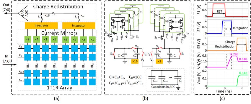
It is also equipped with a buffer called Rifm buffer to store Figure 3: Domino PE: (a) The block diagram of the
received input data in the current cycle. Moreover, Rifm Domino PE, (b) the neuron circuit in the Domino PE, and
has in-tile connections with PE and Rofm. The bits in the (c) the simulation waveform of the PE.
Rifm buffer controlled by an 8-to-1 MUX are sequentially
sent to PE for MAC computations. The buffer size is 8×Nc
bits where Nc is the number of rows in PE (PE consists a 4.5 Domino PE
Nc × Nm ReRAM array which is discussed in Section 4.5). It PE is the computation center that links a Rifm and a Rofm
supports an in-buffer shifting operation with a step size of 64 in the same tile. Fig. 3 (a) shows the architecture of the pro-
or the multiple of 64, which supports the case when the input posed Domino PE, which is composed of a 1T1R crossbar
channels of a layer are less than Nc . A shortcut connection array, current mirrors, two integrators, and a Successive Ap-
from Rifm to Rofm is established to support the situation that proximation Register (SAR) ADC [50]. As shown in Fig. 3
MAC computation is skipped (i.e., the shortcut in a ResUnit). (b), eight single-level 1T1R cells are used to represent one
A counter and a controller in Rifm decide input dataflow 8-bit weight w[7:0] . The voltage on ReRAM is clamped by the
based on the initial configuration. Once Rifm receives input gate voltage and threshold voltage, which will generate two
packets, the counter starts to increment the counter’s value. levels’ of current based on the status of ReRAM and access
The controller chooses to activate MAC computation or sends transistors. Weight bits are divided into two sets (BL7−4 and
4BL3−0 ). In each set, four current mirrors are used to provide described in Eqn. 2 is used to deal with the above-mentioned
the significance for each bit line ( 8k , 4k , 2k , and k, where k is the issue: the Cin × Cout weight matrix is divided into mt × ma
gain to control the integration speed). The output of current smaller matrices Wi j with the dimension of Nc × Nm . The
mirrors is accumulated in the integrator. The higher four bits input vector is divided into mt small slices xi to multiply the
and lower four bits are jointed by the charge redistribution partitioned weight matrices. As shown in Fig. 4 (a), the sum
between two capacitors in the two integrators with a ratio of of the multiplication results within a column of partitioned
16:1. The significance of the input data is also realized by matrices is a slice of output vector y j . The slices of vectors
averaging the charge between integrators and ADC [50]. The are concatenated to produce the complete output.
simulation waveform of the integration and charge sharing
process is shown in Fig. 3 (c). In the initial configuration, x = [x1 , x2 · · · , xmt ]
neural network weights are mapped to ReRAM arrays in PEs,
which will be discussed in detail in Section 5. W11 W12 · · · W1ma
W = ... .. .. ..
. . .
5. DATAFLOW MODEL (2)
Wmt 1 Wmt 2 · · · Wmt ma
We propose “computing-on-the-move” dataflow to reduce
mt
both data movement and data duplication. Below we will in-
y = [y1 , y2 · · · , yma ], y j = ∑ xi Wij
troduce the dataflow in FC layers, CONV layers, and pooling i=1
layers, then reveal how it supports different types of DNN and
achieve high performances. The other “computing-on-the- We propose a mapping scheme for efficient computation
way” schemes such as MAERI [27] and Active-routing [21] in FC layers to efficiently handle partitioned matrix multi-
map computation elements to memory network for near- plication in our tile-based Domino. As shown in Fig. 4 (b),
memory computing and aggregate intermediate results when the partitioned blocks are mapped to mt × ma tiles (mt =
transmitting in a tree adder controlled by a host CPU. In d CNinc e, ma = d CNout
m
e), which is divided into four columns and
contrast, Domino conducts MAC operations in memory. The four rows. The input vectors are transmitted to all ma columns
partial-sums are added up to get group-sums, which are then of tiles. The multiplication results, ¶ to ¹, are added while
stored in the buffer to wait for other group-sums ready for transmitting along the column. The final addition results in
addition. The group-sums are added up when moving along the last tiles of the four columns, U to Z, are small slices of an
the routers controlled by local schedule tables. Domino only output vector. Concatenating the small slices in all columns
transmits data while MAERI/Active-routing contains extra gives the complete partitioned matrix multiplication result.
complex information such as operator and flow states.
5.2 Dataflow in CONV Layers
5.1 Dataflow in FC layers
Based on Eqn. 1, the computation of a pixel in OFM is
the sum of point-wise MAC results in a sliding window.
As shown in Fig. 5, we define the Nm point-wise and row-
wise MAC results as the partial-sum and group-sum, respec-
tively. This figure illustrates our distributed way of adding
partial-sums and timing control of “computing on the move”
(l)
dataflow. Let Pa denote the partial-sum of the l th pixels in
th (b)
the a sliding window and Ga denote the group-sum of the
th th
b row in the a sliding window.
C−1
(l)
Pa = ∑ I[Sx + i][Sy + j][c] × W[i][ j][c]
c=0
C−1 c−1
(b)
Figure 4: The proposed mapping and dataflow in FC lay-
Ga = ∑ ∑ I[Sx + b][Sy + j][c] × W[b][ j][c] (3)
c=0 j=0
ers: (a) the partitioned input vector and weight matrix; K−1
(b) the dataflow to transmit and add multiplication re- O[x][y] =
(b)
sults to a complete MVM result.
∑ Ga
b=0
(l) (b)
In an FC layer, IFMs are flattened to a vector with di- where l = iK + j, and a = xF + y. Pa , Ga , O[x][y], and
mension 1 ×Cin to perform a Matrix-Vector Multiplication W[i][ j][c] ∈ RM . As shown in Fig. 5 (a), K partial-sums (¶,
(MVM) computing with the weights. MVM can be formu- ·, and ¸) can be added up to be a group-sum (U1 ). Fig. 5
lated as y = xW, where x ∈ R1×Cin , y ∈ R1×Cout are input and (b) illustrates how K group-sums (U1 , U2 , and U3 ) are added
output vector, respectively, and W ∈ RCin ×Cout is a weight up to be a complete convolution result U (the same for X, Y,
matrix. Z). U1 , U2 , and U3 are sequentially generated and summed
In most cases, the input and output vector dimensions in up one by one, in different timing and tiles. The group-sums
FC layers are larger than the size of a single crossbar array wait in the buffer for ready of other group-sum, or are evicted
in PE. Therefore, the partitioned matrix multiplication as once they are no longer needed.
5array. As defined in Eqn. 3, a group-sum is the sum of K
partial-sums. We can cluster K tiles mapped into the same
row to a group. We categorize the CONV dataflow into three
types: input dataflow, partial-sum dataflow, and group-sum
dataflow.
The input dataflow. The blue arrows in Fig. 6 (a) illus-
trate the input dataflow in a K 2 × 1 array of tiles. The inputs
are transmitted to an array in rows and flow through Rifms in
K 2 tiles with identical I/O directions. Another type of zigzag
dataflow is demonstrated in Fig. 6 (b) in a K × K array of
tiles. When the input data reach the last tile of a group, Rifm
inverts the flow direction, and the input data are transmitted
to the tile at the adjacent column.
Figure 5: (a) The defined partial-sum and group-sum; (b)
The partial-sum dataflow. The partial-sum dataflow is
The timing and location of how Domino generates OFM
shown in Fig. 6 (c). a represents the first input data of IFM.
with naive dataflow.
At each cycle, input packets are transmitted to the Rifm of
the succeeding tile. Meanwhile, MAC computation in PE
As shown in Fig. 6 (a), the input channels and output is enabled if needed. Take input data a as an example, in
channels of a CONV layer are mapped to the inputs and the the first cycle, a is multiplied with weight A to produce a
outputs of a tile, respectively. If Nc = C and Nm = M, K 2 partial-sum ¶ which will be transmitted by Rofm to the next
points of the filters are mapped to K 2 tiles. In the case that the tile. In the second cycle, a is transmitted to tile whose PE
dimension of a weight matrix exceeds the size of the ReRAM is mapped with weight B. The controller in the Rifm will
crossbar array in PE (Nc ≤ C and Nm ≤ M), the filters are split bypass MAC computation because a only multiplies with A
and mapped to d NCc e × d NMm e tiles. The tiles are placed closely in convolution. In the meanwhile, ¶ is stored in the Rofm
to minimize the data transmission. Likewise, the input vector buffer waiting for addition. In the third cycle, b is multiplied
is split and contained in d NCc e input packets. Adding and with B in PE, and partial-sum · is received by Rofm. Then
¶ is popped out from the Rofm buffer and added with ·.
concatenating MAC results of these PEs will generate the
Generally, partial-sums are added up to be a group-sum U1
same result as the non-split case. This case is similar to the
when transmitting along a group of tiles.
FC dataflow as discussed earlier. When Nc > C, multiple
The group-sum dataflow. Adding group-sums to convo-
points in a filter can be mapped to the same tile to improve
lution results is also a process executed during data trans-
ReRAM cells’ utilization and reduce the energy for data
mission. As shown in Fig. 6 (a) and (b), the orange arrows
movement and partial-sum addition. In such a scenario, the
indicate the group-sum dataflow. Group-sums add up to get
CONV computing is accomplished by the in-buffer shifting
the convolution result U in the last tile of each group. When
operation. In case Nm ≥ 2M, the filters can be duplicated
U1 is generated, it will wait in the third tile until U2 is gen-
inside a tile to maximize parallel computing.
erated in the sixth tile. Then, U1 will be transferred to the
sixth tile to add U2 . Similarly, U1 + U2 waits in the sixth
tile for U3 to generate a complete result U. After all linear
matrix computation, the computation unit in Rofm controlled
by instructions takes effect. An activation function is applied
on the complete convolution result in Rofm in the last tile.
5.3 Synchronization
Because of down sampling in CONV layers, the CONV
steps change with layers. For example, if the pooling filter
size K p = 2 and the pooling filter stride S p = 2, every four
OFM pixels will produce a pooling result. Therefore, the com-
puting speed of the next layer has to be four times slower than
the preceding layer, which will waste the hardware resource
Figure 6: The proposed mapping and dataflow in CONV and severely affect the computing throughput. To maximize
layer: (a) a K 2 × 1 tile array mapping weights in a CONV computation parallelism and throughput, the CONV filters
layer; (b) another type of K × K tiles array mapping need to be duplicated. In other words, the weights of the
weights in a CONV layer; (c) adding a group-sum while preceding filters should be duplicated by four times in the
transmitting MAC results in a group of tiles. above example.
However, a DNN model usually has a few down sampling
As shown in Fig. 6 (a) and (b), each split block is allocated layers. As a result, the number of duplicated tiles may exceed
with an array of tiles that maps weights in a CONV layer. the total number of tiles in Domino. Therefore, a block
The array has multiple mapping typologies, such as K 2 × 1 reuse scheme is proposed for such a situation to alleviate
(mt = K 2 , ma = 1) and K × K (mt = ma = K), in pursuit heavy hardware requirements. Fig. 7 demonstrates our weight
of flexible dataflow and full utilization of tiles in the NoC duplication and block reuse scheme for VGG-11 model used
6tiles in reverse order. As shown in Fig. 8 (a), the first four
rows are transmitted to the block in increasing order. The
fifth row of an IFM flows into the last column of the block.
Group-sum T1 is computed in the third tile when the fourth
row flows through the tile. When the fifth row flows through,
group-sum T2 is computed in the sixth tile. Since T1 and T2
are generated in the same column of a block, inter-column
data transfer is reduced.
The partial-sum dataflow. Fig. 8 (b) and (c) depict the
partial-sum dataflow at a certain cycle and the third cycle
thereafter, respectively. In Fig. 8 (b), partial-sums ¶, ¹, and
¼ are computed in the first tiles of their groups and stored in
the Rofm buffer in their succeeding tiles. After two cycles,
Figure 7: Duplication and reuse scheme in VGG-11 partial-sums ·, º, and ½ are generated in the second tiles
model used in [23], there are three pooling layers before in their groups, which are then added with the stored partial-
L5, L7, and L9. The left axis shows the number of tiles sums ¶, ¹, and ¼, respectively. The computing process is
and duplication, and the right axis shows the number of similar to the dataflow without weight duplication except that
reuses. K group-sums are computed in K columns.
The group-sum dataflow. A group-sum dataflow with
weight duplication aims to reduce the data moving distance
in [23] (CIFAR-10 dataset). There are three pooling layers,
by adding up group-sums locally. Blue and pink arrows
and the CONV steps before these three layers are 64, 16,
indicate the group-sum dataflow in Fig. 8 (a). We take the
and 4. If all layers are synchronized, a total of 892 tiles are
convolution results Q and T for instances. Based on the input
required to map the network. If we reuse the tiles for all
dataflow and partial-sum dataflow, group-sums Q1 and Q2
CONV layers by four times, the speed of the CONV layers
are computed in the first two columns of a block. Thus Q1
will be four times faster than the FC layers. In such a situation,
is transmitted from the first column to the adjacent column
a total of 286 tiles are required to map the network. It can
when it reaches the sixth tile. Q2 is stored in the Rofm buffer
be concluded that there is a trade-off between chip size and
waiting for Q1 . Q2 will be popped out by instruction when
throughput.
Rofm receives Q1 . They will be added up before transmitting
5.4 Dataflow with Weight Duplication along the second column. The pink arrows represent another
situation that the second group-sum is not waiting in Rofm.
Based on the input dataflow, T1 and T2 are computed in the
same column but in two turns of inputs. When T1 reaches the
sixth tile, T2 is not ready yet. Therefore, T1 will be stored in
the Rofm buffer to wait for the fifth row of data to flow into
the tiles. Once T2 is computed in the sixth tile, T1 and T2
are added up to get T1 + T2 . The group-sum dataflow greatly
reduces the data moving distance and frequency.
5.5 Pooling Dataflow
The computation of CONV and FC layers is processed
within Domino blocks, while the computation of the pooling
layer is performed during data transmission between blocks.
Figure 8: The proposed mapping and dataflow in CONV If a pooling layer follows a CONV layer, with pooling filter
layers with weight duplication: (a) each column of tiles is size K p = 2 and pooling stride S p = 2, every four activation re-
assigned with duplicated weights and receives different sults produce a pooling result. Weight duplication situation is
rows of data in IFM; (b) (c) adding partial-sums to be shown in Fig. 9 (b), in every cycle a block produces four acti-
group-sums while transmitting at two cycles. vation results T to Y. When transmitting across tiles, the data
are compared, and the pooling result Z is computed. Fig. 9
(c) shows the block reuse case that activation results are com-
Take weight duplication and reuse into consideration, the puted and stored in the last tile. A comparison is taken when
dataflow should be modified to match such scheme. The over- the next activation result is computed. The Rofm outputs a
all dataflow with weight duplication is illustrated in Fig. 8. In pooling result Z once the comparison of the pooling filter is
this scenario, a block has ma (ma = 4 is the number of dupli- completed. In this case, the computation frequency before
cation in this example) duplicated K 2 × 1 (mt = K 2 ) arrays pooling layers is 4× higher than the succeeding blocks.
of tiles.
The input dataflow. The input dataflow is demonstrated
in Fig. 8 (a): four rows of data of an IFM are transmitted 6. INSTRUCTIONS AND WORKFLOW
through four arrays of tiles in parallel. The massive data Domino is a highly distributed and decentralized archi-
transmission is alleviated by leveraging the spatial locality. tecture and adopts self-controlled instructions, which are
Every ma rows of data are alternatively transferred to the stored in each Rofm. The reason is that Domino tries to
7distributed and local-controlled structure avoids the extra
instruction transmission and external control signals when
processing DNNs.
After cycle-accurate analyses and mathematical derivation,
instructions reveal an attribute of periodicity. During the con-
volution computation, C-type instructions are fetched from
the schedule table and executed periodically. The period p
(p = 2(P +W )) is related to IFM. Within a period, actions are
Figure 9: Output in the last tile: weight duplication or fixed to the given IFM and DNN configurations. Furthermore,
block reuse scheme is used to deal with pooling layer. every port’s behavior exhibits a period of p with a different
beginning time. The control words for each port are stored in
Rofm, and they are generated based on the assumption that
reduce the bandwidth demand for transmitting data or in- the convolution stride is one. When the convolution stride is
structions through whole NoC, and avoid the delay and skew not one, the compiler will shield certain bit in control words
of long-distance signals; meanwhile, localized instructions to “skip” some actions in the corresponding cycles to meet
retain flexibility and compatibility for different DNNs to be the required dataflow controlling. When a Rofm is mapped
processed. and configured to process the last row of a layer in a CNN, it
will generate activation and pooling instructions. Its period is
6.1 Instruction Set related to pooling stride, p = 2S p .
A set of instructions is designed for computing and trans- Once instructions for each Rofm are received and stored,
mitting data automatically and flexibly when dealing with the Rofm is configured to prepare for computation. For a
different DNNs. In Domino, Rofm is responsible for send- given Rofm, when a clock cycle begins, a counter provides
ing packets and accumulating partial-sums and group-sums an index to Rofm to fetch corresponding control words peri-
correctly. Because our packets transmitted through NoC only odically. When the execution of an instruction ends, the state
contain payloads of DNN without any other auxiliary infor- of the current Rofm will be updated.
mation (i.e., a message header, a tail, etc.), there must be an
intuitive way to control the behavior of each Rofm on the 6.3 Workflow
chip. Consequently, we define an instruction set for Domino. After elaborated introduction and illustration of Domino
The instruction consists of several fields, each of which technical details, the overall workflow and processing chain
represents a set of control words for relative ports or buffers, are naturally constructed and revealed. Fig. 10 shows how
as well as the designed actions, as shown in Tab. 2. The Domino works in a sequence to process DNN. These build-
instruction length is 16 bits, including four distinct fields: an ing blocks cover both ideas and implementations mentioned
Rx field, a Function field, a Tx field, and an opcode field. above and integrate them into a whole architecture.
The Rx field takes responsibility for receiving packets from
different ports. The Function field contains sum and buffer 7. EVALUATION
control in C-type, activation function, pooling, and FC layer
This section evaluates Domino’s characterization and per-
control in M-type. The Tx field governs the transmission
formances in detail, including energy efficiency and through-
of one Rofm to four ports. There are two types of opcodes
put. Meanwhile, we compare Domino against other state-of-
bearing two usages. C-type (stands for convolution type)
the-art CIM-based architectures on several prevailing types
denotes the instruction is served for controlling the process
of CNNs to show the proposed architecture and dataflow
during convolution computation, while the M-type is for
advantages.
miscellaneous operations other than convolution, such as
activating and pooling. 7.1 Methodology
First, we specify the configurations of our Domino under
15 11 10 7 6 5 4 1 0
test; second, we describe the experiment setup and bench-
Rx Ctrl. Sum Buffer Tx Ctrl. Opc. C-type marks; then we determine the normalization methods.
Rx Ctrl. Func Tx Ctrl. Opc. M-type
7.1.1 Configuration
The configuration of Domino and its tile is displayed in
Table 2: The instruction format for Domino. There are Tab. 3. Domino adopts silicon-proven ADC in [20], silicon-
two basic types of instructions generated by the compiler proven SRAM array in [43], and the transmission parameters
to handle dataflow correctly. in [4]. The rest of components are simulated by spice or
synthesized by Synopsys DC with a 45 nm CMOS Process
Design Kit (PDK). Domino runs at a step frequency of 10
6.2 Schedule Table MHz for instruction updating. The data transmission fre-
In Domino, instructions in a Rofm should fit both intra- quency is 640 MHz, and the data width is 64 bits. The supply
and inter- block dataflows to support the “computing-on-the- voltage is 1 V. ReRAM’s area information is normalized from
move” procedure. The compiler generates the instruction the silicon-proven result in [30]. In the initialization stage,
table and configuration information for each tile based on each ReRAM cell in a PE is programmed with a 1-bit weight
the initial input data and the DNN structure. The highly value. Eight ReRAM cells make up an 8-bit weight. At
8Figure 10: The workflow of Domino. Domino takes network model, dataset information, and area or power specification
for compilation. The generated schedule tables and weights are mapped into routers and CIM arrays respectively. After
initialization, Domino begins to execute instructions and infer.
Component Descript. Energy/Compo. Area (µm2 ) tent to each comparison object respectively.
ADC 8b×256 1.76 pJ 351.5
Integrator 8b×256 2.13 pJ 568.3 7.1.4 Normalization
Crossbar cell 8b 32.9 fJ 1.62 A variety of CIM models lead to discrepancies of many
PE total Nc ×Nm 48.1 fJ/MAC 341632 attributes that need normalization and scaling. To make a
Buffer 256B×1 281.3 pJ 826.5 fair comparison, we normalize technology nodes and supply
Ctrl. circ. 1 4.1 pJ 1400.6 voltage of digital circuits in each design to 45 nm and 1 V
Rifm total - 2227.1 according to the equations given in [41]. The activations’
Adder 8b×8×2 0.03 pJ/8b 0.07
and weights’ precision is scaled to 8-bit as well. The supply
Pooling 8b×8 7.6 fJ/8b 34.06
voltage of analog circuits is also normalized to 1 V.
Activation 8b×8 0.9 fJ/8b 7.07 7.2 Performance Results
Data buffer 16KiB 281.3 pJ 52896
We evaluate Domino’s Computational Efficiency (CE),
Sched. Table 16b×128 2.2 pJ/16b 826.5
power dissipation, energy consumption, throughput, and exe-
Input buffer 64b×2 17.6 pJ 51.7
cution time for each experiment environment in benchmarks,
Output buffer 64b×2 17.6 pJ 51.7
and compare them with other architectures.
Ctrl. circ. 1 28.5 pJ 2451.2
Rofm total - 53867.1 7.2.1 Overall Performance
Tile total - 0.398 mm2 We evaluate Domino on various DNN models to prove
that its performance can be generalized to different model
Table 3: The configuration information summary for patterns. Tab. 4 shows Domino’s system execution time,
Domino under evaluation. energy consumption, and computational efficiency when it
runs benchmarks with specified configurations. The time and
energy spent on initialization and compilation are not consid-
the same time, each Rifm and Rofm is configured, and the ered. We break down energy into five parts: CIM, on-chip
schedule tables pre-load instructions. Once the configuration data moving, on-chip data memory, other computation, and
of Domino is finished, the instructions are ready for execu- off-chip data accessing. The first one is the energy consumed
tion, and Domino will commence processing DNNs when in PEs related to MAC operations. The latter four are the
the clock cycle starts. energy of peripheral circuits. Domino achieves a peak CE
of 25.92 TOPS/W when running VGG-19 with ImageNet,
7.1.2 Experiment Setup and a valley CE of 19.99 TOPS/W running ResNet-18 with
We select several types of CIM accelerator architectures CIFAR-10. It denotes that the larger the DNN model size,
as the reference, including three silicon-proven architectures the better CE it achieves. The peripheral energy in VGG-19
and another four simulated architectures. The performance only occupies one-third of the total energy. The through-
data and the configuration parameters of the baselines are put of Domino varies with input data size and DNN model.
taken from their papers. The following three experiments are VGG and ResNet models with a small dataset could achieve
conducted: (1) running different architectures with the bench- 6.25E5 inferences/s high throughput. VGG-19 with Ima-
mark DNNs to compare the power efficiency; (2) evaluating geNet dataset still has a throughput of 1.276E4 inferences/s.
the throughput of Domino under different DNNs and input; The high throughput and low peripheral energy of Domino
and (3) estimating PE utilization with various DNN models are benefited from the pipelined “computing-on-the-move”
and PE size. dataflow that fully utilizes the data locality.
7.1.3 Benchmarks 7.2.2 Computational Efficiency
We evaluate Domino using representative DNN models The comparison between Domino and other state-of-the-
like VGG-11 [23], VGG-16, VGG-19 [39], ResNet-18, and art CIM architectures and DNN accelerator is summarized
ResNet-50 [18] as the model benchmarks. The datasets in Tab. 4. The data in the table are either taken or calculated
CIFAR-10 [24] and ImageNet [14] are chosen to be dataset based on the results provided in their papers. The silicon-
benchmarks for evaluation. Then we run benchmarks consis- proven designs usually have low throughput and power con-
9Dataset CIFAR-10 ImageNet
Model VGG-11 ResNet-18 VGG-16 VGG-19 ResNet-50
Architecture [23] Ours [48] Ours [46]*1 [27] Ours [35] [12] Ours [28] Ours
CIM type SRAM ReRAM SRAM ReRAM ReRAM n.a. ReRAM ReRAM ReRAM ReRAM ReRAM ReRAM
Tech. (mm) 16 45 65 45 40 28 45 32 65 45 65 40
VDD (V) 0.8 1 1 1 0.9 n.a. 1 1 1 1 1.2 1
Frequency (MHz) 200 10 100 10 100 200 10 1200 1200 10 40 10
Act. & W. precision 4 8 4 8 8 16 8 16 16 8 8 8
# of CIM array 16 900 4 900 1 n.a. 2500 2560 6400 2500 20352 900
CIM array size (kb) 288 512 16 512 64 n.a. 512 256 4 512 256 512
Area (mm2 ) 25 358.2 9 358.2 9 6 995 5.32 0.99 995 91 358.2
Tapeout/Simulation T S T S T S S S S S S S
Exec. time (us) 128 129.5 1890 203.5 0.67s n.a. 3471 6920 n.a. 3557 n.a. 2397
CIM energy (uJ) 11.47 36.74 36.11 26.44 3700 0 744.1 25000 13000 944.3 130.2 168.3
On-chip data
0.16 2.63 n.a. 3.89 n.a. 36741 46.39 n.a. n.a. 52.81 0.64 16.97
moving energy (uJ)
On-chip memory
5.11 25.41 n.a. 24.21 n.a. 27556 446.4 2310 2180 508.1 71.22 115.41
energy (uJ)
Other comp. (uJ)*2 2.67 0.48 n.a. 0.46 n.a. 50519 8.41 n.a. 1040 9.59 44.96 1.68
Off-chip data
n.a. 0 123.89 0 3690 n.a. 0 5650 4000 0 85.98 0
accessing energy (uJ)
Power (W) 0.17 40.78 0.005 34.38 0.011 0.54 15.89 4.8 0.003 19.33 166 30.84
CE (TOPS/W) 71.39 23.41 6.91 19.99 4.15 0.27 24.84 0.68 3.55 25.92 21 23.14
Normalized*3
9.53 23.41 2.82 19.99 9.24 0.36 24.84 2.73 12.98 25.92 22.46 23.14
CE (TOPS/W)
Throughput (TOPS) 12.14 954.66 0.036 687.26 0.046 0.15 394.7 3.28 0.1 501 3488 713.6
Throughput
0.49 2.67 0.004 1.92 0.005 0.025 0.4 0.62 0.10 0.5 38.33 1.99
(TOPS/mm2 )
inferences/s 7815 6.25E5 n.a. 6.25E5 n.a. n.a. 1.28E4 n.a. n.a. 1.28E4 n.a. 1.02E5
Accuracy(%) 91.51 89.85 91.15 91.57 46 n.a. 70.71 n.a. n.a. 72.38 76 74.89
*1 Adapted and normalized from average statistics. *2 Including CNN related computation like partial sum accumulation, activation functions, pooling operations, etc.
*3 Voltage normalized to 1 V, precision normalized to 8-bit and digital circuit normalized to 45 nm referring to [41].
Table 4: Domino’s evaluation results and comparison under different DNN models.
sumption due to the small chip size. The typical bit width is
only 4-bit because analog computing is difficult to achieve
a high signal-to-noise ratio. It can be seen between the CIM
computing efficiency and the system computing efficiency
that energy consumed by the peripheral circuits for data mov-
ing and memory accessing may still dominate the total power
consumption in most of the design. Benefited from a 16 nm
technology node and tailored DNN model, Jia [23] could
achieve a smaller gap between the CIM computing efficiency
(121 TOPS/W) and the system computing efficiency (71.39
TOPS/W) at 4-bit configuration.
To make a fair comparison among different designs, all
circuits are normalized to 1 V, 8-bit and digital components
are further normalized to 45 nm. From Fig. 11 we can see that
Domino achieves the highest system CE (25.92 TOPS/W),
which is 1.15-9.49× higher than the CIM counterparts. More- Figure 11: Performance comparisons with other archi-
over, Domino has a lower percentage of memory accessing, tectures (a) System computational efficiency after nor-
data transmitting energy (in Tab. 4). The energy breakdown malization; (b) Throughput normalized to each 8-bit
shows that Domino effectively reduces peripheral energy crossbar array cell.
consumption, which is a vital factor in the overall system
performance. The data locality and “computing-on-the-move”
dataflow are very efficient in reducing the overall energy 7.2.3 Throughput
consumption for DNN inference.
Domino has a distinguished advantage over other architec-
As for DNN accelerators, Domino overwhelms MAERI
tures in terms of throughput. The existing architectures need
[27] on CE, which is the representative of conventional digital
to store feature maps and partial-sums to external memory
architecture. The superiority comes not only from the use of
to support the complex dataflow. Furthermore, some de-
CIM but also from “computing-on-the-move” dataflow.
signs also have to access external memory to update weights
for different layers. In Domino, the weights of the DNN
10are all stored in crossbar arrays in the initial configuration.
Layer synchronization with weight duplication and block
reuse scheme is further proposed to maximize the parallel
computing speed of inference.
The chip size and the number of memory cells greatly af-
fect the overall throughput of a system, and different memory
type has different memory size (i.e., ReRAM and SRAM).
As shown in Tab. 4, the area normalized throughput of [48]
is 0.004 TOPS/mm2 due to the small array size and 65 nm
technology node. With a larger crossbar array size and 16 nm
technology node, [23] achieves 0.486 TOPS/mm2 . Our pro-
posed scheme can achieve up to 2.67 TOPS/mm2 throughput, Figure 12: Utilization rates over all layers in four DNN
which is better than the state-of-the-art schemes except [28]. models considering three PE crossbar configurations.
The high density of [28] is due to the transistor-less cross-
bar array estimated on 20nm technology node, which often
suffers from the write sneak path issue and is very difficult is a ReRAM-based accelerator that uses ReRAM crossbars to
to program the ReRAM cells to the desired state. Therefore, store weights and eDRAM to store feature maps, which are
we normalize the throughput to an 8-bit cell, which reflects organized by routers and H-trees. Pipelayer [40] stores both
both throughput and PE utilization. As shown in Fig. 11 filters and feature maps in ReRAM crossbars and computes
(b), our design achieves 16.19 MOPS/8-b-cell throughput, them in the pipelined dataflow. The interface between analog
which is 3.10× higher than TIMELY and 270× higher than domain and digital domain also contributes to high power
CASCADE. Although [47] supports zero-skipping and im- consumption. [50] proposes a binary input pattern for CIM,
plements a ping-pong CIM for computing while refreshing, instead of a high power consumption DAC, to reduce the
and [23] provides various mapping strategies to improve the interface energy. In this way, both computing efficiency and
throughput, Domino still outperforms them by 7.36× and reliability are improved. CASCADE [12] applies the signifi-
1.57×, respectively. The high throughput of Domino comes cance of the bit lines in the analog domain to minimize A/D
from the synchronization, the weight pre-loading, the data conversions, thus enhancing power efficiency. TIMELY [28]
locality, and the pipelined dataflow to reduce the computing also focuses on analog current adder to increase the CIM
latency while maximizing the parallelism. block size, TDC and DTC to reduce the power consumption,
and input data locality to reduce data movement. However,
7.2.4 Utilization Rates the uncertainty caused by the clock jitter and the time vari-
The size of the crossbar array greatly affects the CIM ation caused by the complex RRAM crossbar network will
power efficiency and cell utilization in PEs. Fig. 12 de- greatly reduce the ENOB of the converters. Moreover, the
picts the crossbar array utilization over all layers in four large sub-chip and weight duplication inside the crossbar ar-
neural network models: VGG-11, VGG-16, ResNet-18, and ray also significantly reduce the utilization of the CIM arrays.
ResNet-50 with three crossbar array configurations (128 × Till now, most of the designs don’t provide on-chip control
128, 256 × 256, and 512 × 512). Though the mapping strate- circuits to maintain the complicated dataflow. Therefore, the
gies in Domino have improved cell utilization in PEs, they feature maps or partial-sums have to be stored on the external
still have low utilization in the first few layers because the memory and controlled by additional processors to transform
input and output channels are much less than the side length the feature maps’ flow and synchronize the computing la-
of the crossbar array. The average utilization of four models tency of different data paths. Accessing feature maps and
is 98%, 96%, 93%, and 92% when using a 128×128 crossbar partial-sums have been the leading energy consumption in
array. The utilization is reduced to 90%, 89%, 86% and 79% most designs. Reducing the data movement energy has been
using a 256×256 crossbar array, and 75%, 76%, 67% and one of the most important research topics to design CIM
54% with a 512×512 crossbar array. Lower utilization in processors.
ResNet comes from its architecture that layers with small
channels are prevalent. Though a smaller crossbar array has 9. CONCLUSION
higher utilization, it sacrifices the CIM computing efficiency,
which is 31.4 TOPS/W, 41.58 TOPS/W, and 49.38 TOPS/W This paper has presented a tailored Network-on-Chip ar-
at these three configurations. Therefore, it is a balance be- chitecture called Domino with highly localized inter- and
tween utilization and computational efficiency. intra-memory computing for DNNs. The key contribution
and innovation can be concluded as follows: Domino (1)
changes conventional NoC tile structure by using two dual
8. RELATED WORK routers for different usages aimed at DNN processing, and en-
Various CIM architectures have been proposed to adopt abling architecture to substitute PE for different types of CIM
different designs, computing strategies, and architectures. arrays, (2) constructs highly distributed and self-controlled
SRAM- or DARAM-based CIM chips usually need to update processor architecture, proposes efficient matching dataflow
weights by accessing off-chip memory [10, 17, 23, 47], re- to perform “computing-on-the-move”, and (3) defines a set of
sulting in high energy consumption and latency. [23] utilizes instructions for routers, which is executed periodically to pro-
1152 input rows to fit a 3×3 convolution filter, which will face cess DNNs. Benefiting from such design, Domino has unique
low cell utilization in other DNN configurations. ISAAC [38] features with respect to (1) eliminating data access to memory
11during one single inference, (2) minimizing data movement [13] M. Davies, N. Srinivasa, T. Lin, G. Chinya, Y. Cao, S. H. Choday,
on-chip, (3) achieving high computational efficiency and G. Dimou, P. Joshi, N. Imam, S. Jain, Y. Liao, C. Lin, A. Lines, R. Liu,
D. Mathaikutty, S. McCoy, A. Paul, J. Tse, G. Venkataramanan,
throughput. Compared with the competitive architectures, Y. Weng, A. Wild, Y. Yang, and H. Wang, “Loihi: A neuromorphic
Domino has achieved 1.15-to-9.49× power efficiency im- manycore processor with on-chip learning,” IEEE Micro, vol. 38,
no. 1, pp. 82–99, 2018.
provement and improved the throughput by 1.57-to-12.96×
over several current advanced architectures [2] [49] [30]. [14] J. Deng, W. Dong, R. Socher, L. Li, Kai Li, and Li Fei-Fei, “Imagenet:
A large-scale hierarchical image database,” in 2009 IEEE Conference
on Computer Vision and Pattern Recognition, 2009, pp. 248–255.
REFERENCES [15] A. Firuzan, M. Modarressi, M. Daneshtalab, and M. Reshadi,
[1] F. Akopyan, J. Sawada, A. Cassidy, R. Alvarez-Icaza, J. Arthur, “Reconfigurable network-on-chip for 3d neural network accelerators,”
P. Merolla, N. Imam, Y. Nakamura, P. Datta, G. Nam, B. Taba, in 2018 Twelfth IEEE/ACM International Symposium on
M. Beakes, B. Brezzo, J. B. Kuang, R. Manohar, W. P. Risk, Networks-on-Chip (NOCS), 2018, pp. 1–8.
B. Jackson, and D. S. Modha, “Truenorth: Design and tool flow of a
65 mw 1 million neuron programmable neurosynaptic chip,” IEEE [16] D. Fujiki, S. Mahlke, and R. Das, “In-memory data parallel processor,”
Transactions on Computer-Aided Design of Integrated Circuits and SIGPLAN Not., vol. 53, no. 2, p. 1–14, Mar. 2018. [Online]. Available:
Systems, vol. 34, no. 10, pp. 1537–1557, 2015. https://doi.org/10.1145/3296957.3173171
[2] M. Bavandpour, M. R. Mahmoodi, and D. B. Strukov, [17] R. Guo, Z. Yue, X. Si, T. Hu, H. Li, L. Tang, Y. Wang, L. Liu, M. F.
“Energy-efficient time-domain vector-by-matrix multiplier for Chang, Q. Li, S. Wei, and S. Yin, “15.4 a 5.99-to-691.1tops/w
neurocomputing and beyond,” IEEE Transactions on Circuits and tensor-train in-memory-computing processor using
Systems II: Express Briefs, vol. 66, no. 9, pp. 1512–1516, 2019. bit-level-sparsity-based optimization and variable-precision
quantization,” in 2021 IEEE International Solid- State Circuits
[3] M. Besta, S. M. Hassan, S. Yalamanchili, R. Ausavarungnirun, Conference (ISSCC), vol. 64, 2021, pp. 242–244.
O. Mutlu, and T. Hoefler, “Slim noc: A low-diameter on-chip network
topology for high energy efficiency and scalability,” SIGPLAN Not., [18] K. He, X. Zhang, S. Ren, and J. Sun, “Deep residual learning for
vol. 53, no. 2, p. 43–55, Mar. 2018. [Online]. Available: image recognition,” 06 2016, pp. 770–778.
https://doi.org/10.1145/3296957.3177158 [19] J. Hu, L. Shen, and G. Sun, “Squeeze-and-excitation networks,” in
[4] V. Catania, A. Mineo, S. Monteleone, M. Palesi, and D. Patti, 2018 IEEE/CVF Conference on Computer Vision and Pattern
“Cycle-accurate network on chip simulation with noxim,” ACM Trans. Recognition, 2018, pp. 7132–7141.
Model. Comput. Simul., vol. 27, no. 1, Aug. 2016. [Online]. Available: [20] Y. Hu, C. Shih, H. Tai, H. Chen, and H. Chen, “A 0.6v
https://doi.org/10.1145/2953878 6.4fj/conversion-step 10-bit 150ms/s subranging sar adc in 40nm
[5] L. Chang, X. Ma, Z. Wang, Y. Zhang, Y. Ding, W. Zhao, and Y. Xie, cmos,” in 2014 IEEE Asian Solid-State Circuits Conference (A-SSCC),
“Dasm: Data-streaming-based computing in nonvolatile memory 2014, pp. 81–84.
architecture for embedded system,” IEEE Transactions on Very Large [21] J. Huang, R. Reddy Puli, P. Majumder, S. Kim, R. Boyapati, K. H.
Scale Integration (VLSI) Systems, vol. 27, no. 9, pp. 2046–2059, 2019. Yum, and E. J. Kim, “Active-routing: Compute on the way for
[6] K.-C. J. Chen, M. Ebrahimi, T.-Y. Wang, and Y.-C. Yang, “Noc-based near-data processing,” in 2019 IEEE International Symposium on High
dnn accelerator: A future design paradigm,” in Proceedings of the 13th Performance Computer Architecture (HPCA), 2019, pp. 674–686.
IEEE/ACM International Symposium on Networks-on-Chip, ser. [22] M. Imani, S. Gupta, Y. Kim, and T. Rosing, “Floatpim: In-memory
NOCS ’19. New York, NY, USA: Association for Computing acceleration of deep neural network training with high precision,” in
Machinery, 2019. [Online]. Available: 2019 ACM/IEEE 46th Annual International Symposium on Computer
https://doi.org/10.1145/3313231.3352376 Architecture (ISCA), 2019, pp. 802–815.
[7] W. Chen, K. Li, W. Lin, K. Hsu, P. Li, C. Yang, C. Xue, E. Yang, [23] H. Jia, M. Ozatay, Y. Tang, H. Valavi, R. Pathak, J. Lee, and N. Verma,
Y. Chen, Y. Chang, T. Hsu, Y. King, C. Lin, R. Liu, C. Hsieh, K. Tang, “15.1 a programmable neural-network inference accelerator based on
and M. Chang, “A 65nm 1mb nonvolatile computing-in-memory scalable in-memory computing,” in 2021 IEEE International Solid-
reram macro with sub-16ns multiply-and-accumulate for binary dnn ai State Circuits Conference (ISSCC), vol. 64, 2021, pp. 236–238.
edge processors,” in 2018 IEEE International Solid - State Circuits
Conference - (ISSCC), 2018, pp. 494–496. [24] A. Krizhevsky, “Learning multiple layers of features from tiny images,”
University of Toronto, 05 2012.
[8] Y. Chen, T. Yang, J. Emer, and V. Sze, “Eyeriss v2: A flexible
accelerator for emerging deep neural networks on mobile devices,” [25] H. Kwon,, A. Samajdar, and T. Krishna, “A communication-centric
IEEE Journal on Emerging and Selected Topics in Circuits and approach for designing flexible dnn accelerators,” IEEE Micro, vol. 38,
Systems, vol. 9, no. 2, pp. 292–308, 2019. no. 6, pp. 25–35, 2018.
[9] Y.-H. Chen, J. Emer, and V. Sze, “Eyeriss: A spatial architecture for [26] H. Kwon, A. Samajdar, and T. Krishna, “Rethinking nocs for spatial
energy-efficient dataflow for convolutional neural networks,” in neural network accelerators,” in Proceedings of the Eleventh
Proceedings of the 43rd International Symposium on Computer IEEE/ACM International Symposium on Networks-on-Chip, ser.
Architecture, ser. ISCA ’16. IEEE Press, 2016, p. 367–379. [Online]. NOCS ’17. New York, NY, USA: Association for Computing
Available: https://doi.org/10.1109/ISCA.2016.40 Machinery, 2017. [Online]. Available:
https://doi.org/10.1145/3130218.3130230
[10] Z. Chen, X. Chen, and J. Gu, “15.3 a 65nm 3t dynamic analog
ram-based computing-in-memory macro and cnn accelerator with [27] H. Kwon, A. Samajdar, and T. Krishna, “Maeri: Enabling flexible
retention enhancement, adaptive analog sparsity and 44tops/w system dataflow mapping over dnn accelerators via reconfigurable
energy efficiency,” in 2021 IEEE International Solid- State Circuits interconnects,” in Proceedings of the Twenty-Third International
Conference (ISSCC), vol. 64, 2021, pp. 240–242. Conference on Architectural Support for Programming Languages and
Operating Systems, ser. ASPLOS ’18. New York, NY, USA:
[11] Y. D. Chih, P. H. Lee, H. Fujiwara, Y. C. Shih, C. F. Lee, R. Naous, Association for Computing Machinery, 2018, p. 461–475. [Online].
Y. L. Chen, C. P. Lo, C. H. Lu, H. Mori, W. C. Zhao, D. Sun, M. E. Available: https://doi.org/10.1145/3173162.3173176
Sinangil, Y. H. Chen, T. L. Chou, K. Akarvardar, H. J. Liao, Y. Wang,
M. F. Chang, and T. Y. J. Chang, “16.4 an 89tops/w and 16.3tops/mm2 [28] W. Li, P. Xu, Y. Zhao, H. Li, Y. Xie, and Y. Lin, “Timely: Pushing
all-digital sram-based full-precision compute-in memory macro in data movements and interfaces in pim accelerators towards local and
22nm for machine-learning edge applications,” in 2021 IEEE in time domain,” in Proceedings of the ACM/IEEE 47th Annual
International Solid- State Circuits Conference (ISSCC), vol. 64, 2021, International Symposium on Computer Architecture, ser. ISCA ’20.
pp. 252–254. IEEE Press, 2020, p. 832–845. [Online]. Available:
https://doi.org/10.1109/ISCA45697.2020.00073
[12] T. Chou, W. Tang, J. Botimer, and Z. Zhang, “Cascade: Connecting
rrams to extend analog dataflow in an end-to-end in-memory [29] Q. Liu, B. Gao, P. Yao, D. Wu, J. Chen, Y. Pang, W. Zhang, Y. Liao,
processing paradigm,” in Proceedings of the 52nd Annual IEEE/ACM C. Xue, W. Chen, J. Tang, Y. Wang, M. Chang, H. Qian, and H. Wu,
International Symposium on Microarchitecture, ser. MICRO ’52. “33.2 a fully integrated analog reram based 78.4tops/w
New York, NY, USA: Association for Computing Machinery, 2019, p. compute-in-memory chip with fully parallel mac computing,” in 2020
114–125. [Online]. Available: IEEE International Solid- State Circuits Conference - (ISSCC), 2020,
https://doi.org/10.1145/3352460.3358328 pp. 500–502.
12You can also read