A comparison of baleen whale density estimates derived from overlapping satellite imagery and a shipborne survey - Nature
←
→
Page content transcription
If your browser does not render page correctly, please read the page content below
www.nature.com/scientificreports
OPEN A comparison of baleen whale
density estimates derived
from overlapping satellite imagery
and a shipborne survey
C. C. G. Bamford1,2*, N. Kelly3, L. Dalla Rosa4, D. E. Cade5,6, P. T. Fretwell1, P. N. Trathan1,
H. C. Cubaynes1, A. F. C. Mesquita4, L. Gerrish1, A. S. Friedlaender6 & J. A. Jackson1
As whales recover from commercial exploitation, they are increasing in abundance in habitats that
they have been absent from for decades. However, studying the recovery and habitat use patterns
of whales, particularly in remote and inaccessible regions, frequently poses logistical and economic
challenges. Here we trial a new approach for measuring whale density in a remote area, using Very-
High-Resolution WorldView-3 satellite imagery. This approach has capacity to provide sightings data
to complement and assist traditional sightings surveys. We compare at-sea whale density estimates
to estimates derived from satellite imagery collected at a similar time, and use suction-cup archival
logger data to make an adjustment for surface availability. We demonstrate that satellite imagery
can provide useful data on whale occurrence and density. Densities, when unadjusted for surface
availability are shown to be considerably lower than those estimated by the ship survey. However,
adjusted for surface availability and weather conditions (0.13 whales per km2, CV = 0.38), they fall
within an order of magnitude of those derived by traditional line-transect estimates (0.33 whales per
km2, CV = 0.09). Satellite surveys represent an exciting development for high-resolution image-based
cetacean observation at sea, particularly in inaccessible regions, presenting opportunities for ongoing
and future research.
Gathering data on cetacean distribution and densities has traditionally employed visual observers operating
from various platforms, typically either ships, aircraft or l and1–5. Much of our understanding about baleen whale
population recovery and ecology depends on these methods6–8. In oceanic regions close to population centres,
these methods are often used to monitor regional population d ensities8–10. However, regular applications of these
methods are often constrained in remote, inaccessible regions, where their use represents a significant logisti-
cal and financial commitment11. Consequently, such surveys are infrequent, making monitoring of population
trends more challenging.
In the Southern Ocean, the only comprehensive surveys south of 60° S (i.e. the putative summer foraging area
for a range of cetacean species) were those undertaken by the International Whaling Commission (IWC) dur-
ing the International Decade of Cetacean Research and the Southern Ocean Whale Ecosystem Research (IDCR
SOWER) surveys, between 1978/9 and 2003/4. These surveys circumnavigated the continent three times, and
based on these data Southern Ocean baleen whale recovery trends have been e stimated6,12,13. However, small-
scale, sometimes ad hoc studies are far more common. These are generally biased towards the most accessible
regions of the Southern Ocean14, the Western Antarctic Peninsula3,4,15–18, with more limited studies also con-
rc19, Weddell S ea20 and limited areas of East A
ducted in the Scotia A ntarctica21,22. The Southern Ocean represents
1
British Antarctic Survey, High Cross, Madingley Road, Cambridge CB3 0ET, UK. 2University of Southampton,
University Road, Southampton SO17 1BJ, UK. 3Australian Antarctic Division, Department of Agriculture,
Water and the Environment, Australian Government, Channel Highway, Kingston 7050, Australia. 4Laboratório
de Ecologia e Conservação da Megafauna Marinha, Instituto de Oceanografia, Universidade Federal do Rio
Grande-FURG, Av. Itália km.8, Rio Grande, RS 96203‑900, Brazil. 5Hopkins Marine Station, Stanford University,
120 Ocean View Blvd, Pacific Grove, CA 93950, USA. 6Institute for Marine Sciences, University of California Santa
Cruz, 115 McAllister Way, Santa Cruz, CA 95006, USA. *email: conord48@bas.ac.uk
Scientific Reports | (2020) 10:12985 | https://doi.org/10.1038/s41598-020-69887-y 1
Vol.:(0123456789)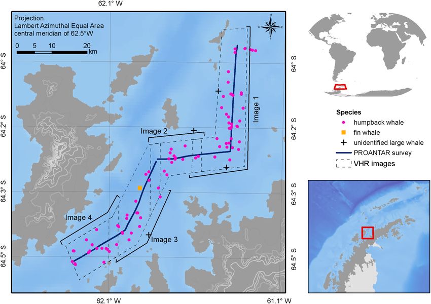
www.nature.com/scientificreports/
a region, amongst others globally11, that would benefit from further research into the structure and functioning
of the whole ecosystem23.
Recent developments in the use of Unmanned Aerial Systems (UAS) for surveys suggest that it may be pos-
sible to monitor and detect marine mammals r emotely24–26, without the limiting factors associated with crewed
flights26. Collection of aerial imagery also minimises the effects of animal movement (attraction/avoidance)27,
associated with traditional ship-based survey p latforms1. Additionally, sighting data collected on traditional
in situ observer-based platforms can be impacted by observer f atigue26, whereas by generating a permanent
record of a sighting, an image-based survey allows the analyst to revisit data. Image-based surveys therefore
reduce the reliance of the data analyst on near-instantaneous observer decisions, a key source of perception
bias for traditional distance sampling surveys. However, the cost of long-range UAS platforms and surveys
currently far exceeds that of comparable aerial platforms, both for d eployment25, and subsequent a nalysis28.
An alternative approach for collecting overhead imagery and detecting whales at sea has been provided by the
development of sub-metre or Very-High-Resolution (VHR) satellite imagery. Since the early 2000′s, applications
of VHR imagery have been mainly developed for terrestrial species and environments, with only a few studies
focussing on large marine species at sea29–32. Terrestrially focussed VHR studies have proven valuable for study
species in remote regions, particularly the high latitudes33–40, where contrast between the target species and their
visually-homogeneous environment makes their detection e asier41. Comparisons between traditional methods
and image-based techniques have only been undertaken in a few cases, notably in the high latitudes, where
Emperor penguins Aptenodytes forsteri34, elephant seals Mirounga leonina40, wandering Diomedea exulans and
royal albatross D. sanfordi33, and polar bears Ursus maritimus36,42 have been examined. All of these studies have
demonstrated that VHR counts were comparable to traditional ground-based counts, highlighting the merit of
this novel platform for remote ecological observations. However, to date, ground-to-space comparisons have been
exclusively terrestrial, and there have been no attempts to compare animal densities estimated from traditional
at-sea surveys to those obtained through VHR image analysis.
Applying VHR imagery for conservation research is in its infancy. However, the ability to rapidly and repeat-
edly task a satellite to acquire images from anywhere on the planet is a distinct advantage in ecological research,
particularly given the resampling limitations facing traditional survey methods in remote regions stemming from
the logistics and associated cost of such surveys. The emergence of this technique offers the possibility to hindcast
analyses back to ca.2009, and the launch of the WorldView-2 satellite (when the resolution arguably became fine
enough to discriminate features at s ea30), and examine densities over the past decade in regions where imagery
is available. The present study aims to provide the first assessment of space-borne, VHR image-derived density
estimates for whales using this area, compared to those obtained from a traditional ship line-transect survey, in
a region where traditional surveys are often constrained. We selected a remote region where species composition
is dominated by a single species, and local geomorphology provides sheltered, low sea-state surface conditions
well suited to satellite imagery analysis30. The region is the Gerlache Strait, Western Antarctic Peninsula (WAP),
63° 45′ S to 65° 00′ S, an area known to be a significant summer feeding area for cetaceans; notably humpback
whales Megaptera novaeangliae15,43, where they typically comprise > 80% of sightings15,16.
Results
Ship survey. Total line effort considered for this study was 90.7 km, with an effective half strip width esti-
mated to be 3.1 km (CV = 0.07). A total of 90 groups (185 individuals; 95.7% humpback, n = 177, 85 groups;
2.7% unidentified large whale, n = 5, 4 groups; 1.6% fin, n = 3, 1 group) were encountered. Average group size
was estimated as 2.06 individuals (CV = 0.01). Right truncation at 5% of the maximum perpendicular detection
distance was tested but did not improve the fit of the models, so was not implemented. A half-normal key with
no covariates best fit the data (CvM p = 0.376) (Fig. 1), but multiple models were within 2 AIC units of each other
(Table 1). Parameter estimates were checked to rule out implausible models, and the most parsimonious model
was selected. Along-track density was estimated at 0.33 whales per k m2 (95%, CV 0.09).
VHR image analysis. Following manual scanning and classification of the images by the main observer
(O1), a total of 18 “definite”, 21 “probable” and 146 “unclassified” features of interest (FOIs) were identified. A
subset (n = 37, 20%) of these identified features was passed to three independent reviewers (R1–R3) for classifi-
cation. Their scores were then compared to those of O1. The deviation between the FOIs scored by O1 and the
average of the R1, R2, and R3 was less than 1 (mean = − 0.31, median − 0.33), and the associated variance of these
averaged reclassifications spanned both above and below O1 classifications (Fig. S1), suggesting close concord-
ance overall. No adjustment was therefore made to the FOI scores for O1 overall. The proportion of whales clas-
sified as “definite” and “probable” by O1 was 0.27, which was identical to the averaged proportion obtained by
reviewers R1–R3, although there was clearly substantial variation in reviewer scoring (Fig. S2). The proportions
of whales in each focal category were as binomial random variables, and standard errors were calculated for the
proportion of FOIs classified as “definite” (SE = 0.02), “probable” (SE = 0.023), “definite and probable” (SE = 0.03)
and “unclassified" (SE = 0.03). Coefficients of variation (CV) derived from these estimates are shown in Table 2.
To account for availability bias, an adjustment of 0.34 (CV = 0.35) was applied derived from archival suction
cup data collected in the same geographic area and time. Once adjusted for availability bias, and associated
observer classification uncertainty, density was estimated at 0.12 whales per km2 (CV = 0.38). At this stage, satel-
lite image-based densities for the whole region were lower than ship-based densities by a factor of 2.8.
Apparent sea state was recorded during the scanning and classification process. There was a marked increase
in sea state from the north to the south of the study area (Fig. 2). We found that it was both easier to spot and
classify FOIs in images with good to average sea states (i.e. calmer waters), which enable the FOIs to be clearly
differentiated from the surface. FOIs classified as either “definite” or “probable” comprised 0.23 (SE = 0.03) for
Scientific Reports | (2020) 10:12985 | https://doi.org/10.1038/s41598-020-69887-y 2
Vol:.(1234567890)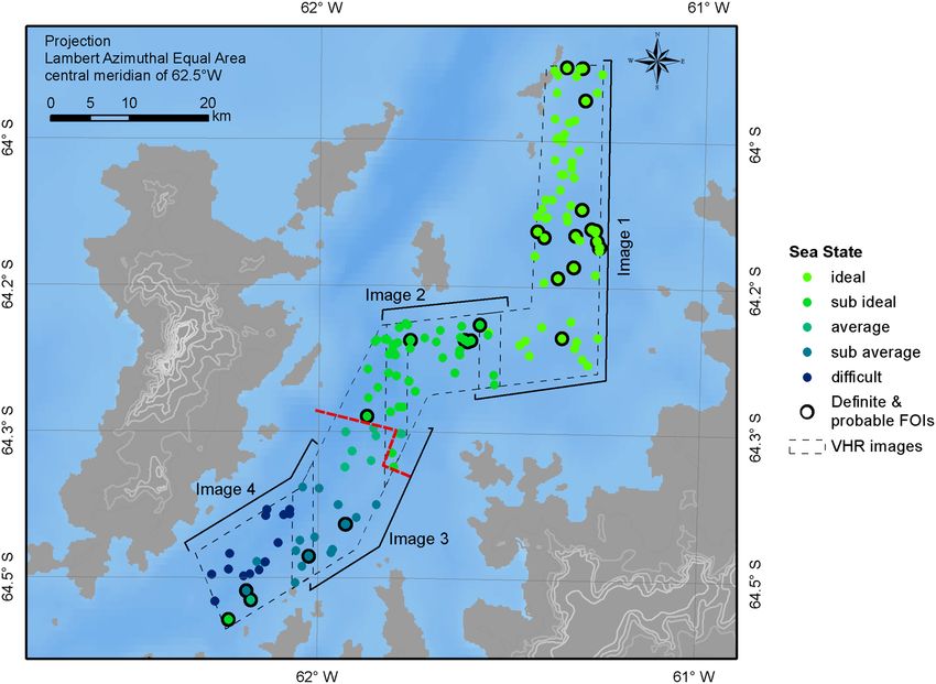
www.nature.com/scientificreports/
Figure 1. Half-normal model detection function with no adjustments and no covariates fitted to the
perpendicular detection distances from the ship-borne line transect survey data.
Model Key Formula CvM p-value P̂a se P̂a AIC
1 half-normal ~1 0.376 0.447 0.031 0.000
5 half-normal ~ sightability 0.403 0.443 0.033 0.759
6 hazard-rate ~1 0.816 0.398 0.054 0.783
7 hazard-rate ~ Beaufort 0.949 0.317 0.061 1.002
2 half-normal ~ Beaufort 0.332 0.444 0.032 1.175
3 half-normal ~ visibility 0.537 0.434 0.034 2.053
10 hazard-rate ~ sightability 0.912 0.394 0.055 2.468
8 hazard-rate ~ visibility 0.957 0.071 0.086 3.161
4 half-normal ~ Beaufort + visibility 0.530 0.433 0.035 3.717
9 hazard-rate ~ Beaufort + visibility 0.963 0.078 0.091 3.867
Table 1. Summary outputs of the fitted detection function models. Headings shortened represent: CvM,
Crammer-von Mises test p-values; P̂a , the average detectability; and se P
a, the standard error of P̂a. Models
listed in order of AIC.
Class Density (km2) CV Density adjusted for availability bias (km2) CV
Definite 0.02 0.22 0.05 0.41
Probable 0.02 0.21 0.06 0.40
Unclassified 0.15 0.14 0.44 0.35
Definite and probable 0.04 0.14 0.12 0.38
Definite and probable (calmer waters) 0.04 0.15 0.13 0.38
Definite and probable (rougher waters) 0.02 0.47 0.05 0.58
Table 2. Whale density estimated using satellite imagery in the Gerlache Strait, and adjusted for availability
bias. Raw, unadjusted densities provided alongside combined “Definite + Probable” unadjusted densities.
Densities for all classifications provided post availability bias adjustment of 0.34, along with estimated CV
values. Densities provided on data from the whole image, and by image quality (i.e. rougher/calmer waters).
Scientific Reports | (2020) 10:12985 | https://doi.org/10.1038/s41598-020-69887-y 3
Vol.:(0123456789)www.nature.com/scientificreports/
Figure 2. Sea state associated with each classified feature of interest (FOI) identified in the satellite imagery
(coloured dots). FOIs surrounded by a black ring indicate those classified as either “definite” or “probable” whale
signs. Red dotted line indicates the approximate position where the sea state transitioned from above (north of
the line) to below average (south of the line). Maps were created by the authors in ESRI ArcGIS v10.6 https://
www.esri.com.
the calmer regions, versus 0.12 (SE = 0.06) for the rough water regions in the south of the study area. Were den-
sity to be calculated by grouping regions based on image quality, calmer regions (classified as good to average
sea states) totalled 635 k m2, and corresponded to a density of 0.04 whales per k m2 (CV = 0.15); 0.13 whales per
km2 (CV = 0.38) once adjusted for surface availability. Rougher regions (classified as sub-average and poor sea
states) totalled 336 km2 and contained 0.02 whales per km2 (CV = 0.47); 0.05 whales per k m2 (CV = 0.58) once
adjusted for surface availability (Fig. 2, Table 2). Comparing between the ship and the satellite estimate from
the calmer waters revealed that satellite estimates underestimated density by a factor of 2.5, and rougher regions
were lower by a factor of 6.3.
Discussion
Here we tested the capacity of VHR imagery to provide estimates useful for monitoring whale distribution and
densities, using a direct comparison with a ship-based line transect survey to gauge the relative sighting rates
obtained by the satellite platform in comparison to that of the ship. Our results show that density estimates
derived from satellite imagery (0.13 whales per km2, CV = 0.38—taken from calm waters) are approximately 0.39
of those estimated from the ship-based survey (0.33 whales per km2, CV = 0.09); an encouraging result suggesting
that data from satellite imagery has potential to detect whales at similar levels to a traditional survey method.
These results match our expectation that image derived densities would be lower than that of the ship-survey,
with the instantaneous nature of the image acquisition on the satellite platform likely a strong driver of these
differences, in addition to limitations in image resolution and the potential for random fluctuations in local whale
densities during the time between acquisition of satellite images and the vessel-based survey. However they also
demonstrate that satellite surveys have sufficient whale detection capacity that they can provide a complementary
approach to monitoring whale presence in remote regions where regular surveys are difficult.
In setting up this study, we chose an area that (1) is of specific scientific interest in terms of whales; (2) is
remote and relatively difficult to access, but has had some whale survey effort; (3) where the environmental condi-
tions are changing; and (4) where whale density and habitat use patterns are required to understand population
Scientific Reports | (2020) 10:12985 | https://doi.org/10.1038/s41598-020-69887-y 4
Vol:.(1234567890)www.nature.com/scientificreports/
recovery from exploitation and spatial overlap with the regional fishery for Antarctic krill. We focused on an area
where one whale species very strongly predominates (humpback whales) in order that our results have poten-
tial use for inference about the density patterns of this species, and as there is a smaller likelihood that species
mis-identification would introduce bias. We also chose a sea channel which is relatively sheltered, reducing the
likelihood of turbulent sea conditions (particularly wind on sea), which can make satellite images useless for
survey. Our site selection considerations highlight the limitations still facing development of VHR as a platform,
and we consider these limitations and next steps to address them in the following sections. We propose that
this method can be used to investigate spatial and temporal patterns of whale distribution and densities, sup-
plementing existing methods, providing that the limitations of this new method are carefully considered during
design and implementation.
Weather conditions, specifically the sea state, impact detectability of whales at sea. Sea state is known to influ-
ence the ability of observers to detect animals, with worsening conditions reducing the detection probability.
Consequently, effort is typically halted when conditions exceed a predefined limit. In all at-sea surveys, sea state
increases the likelihood that the assumption of perfect detection on the track line will be violated. If detection
off the track line is impacted by environmental conditions, inclusion of covariates in the detection function can
take account of this b ias44 (up to a cut off, normally 5). However, if poor sighting conditions impact detection
on the track line, alternative methods such as a double-observer/platform study or a mark recapture approach
can be implemented to account for and quantify this bias. For an image-based survey, poorer weather conditions
will also reduce the ability of the observer to differentiate FOIs from background noise (i.e. breaking waves,
wind lines, etc.)30. This results in fewer features being identified, and lower reported densities. Poor sea state,
and associated wind conditions, typically ground aerial surveys, whether manned or UAS-based, or force them
to be aborted inflight. Here we show that worsening sea states in the south of the study area on the day that the
image was taken (Fig. 2), correspond to lower perceived and estimated densities in these regions. Compared to the
northern area, the surface conditions of the southern image were less conducive to the visual detection of FOIs,
showing an increased frequency of white-caps and wind lines, possibly because this region is prone to katabatic
winds sweeping into the channel. Densities in the south of the survey area, where the sea state was poorer, were
0.4 of those from calmer regions (0.05 versus 0.13 whales per k m2, CV = 0.58 and 0.38, respectively, Table 2). To
address this effect in the future, an adapted version of a Mark-Recapture Distance Sampling (MRDS) analysis,
such as45 using multiple observers to review images33, could be applied to assess variations in detectability as a
function of covariates (i.e. sea state), and investigate the impact of perception bias on whale detection. However,
to accurately parameterise a multi-covariate model, several tens, if not hundreds of whale detections would be
needed. Another approach could be to collect multiple images of the same area very close in time (within several
seconds to a minute of each other), to quantify the variation in whale detections according to sea state when
variation in true whale density is likely to be negligible. In the present study, density comparisons were made
using data from the northern (calmer) portion of the imagery only (0.13 whales per k m2, CV = 0.38, Table 2).
When planning satellite imagery analysis, species composition of the focal area needs to be carefully consid-
ered, because at present this approach has very limited capacity to differentiate between species when compared
to in situ surveys, due to the resolution of the images (~ 30 cm in this study). Our density estimates most likely
reflect the density of humpback whales using the area of the Gerlache Strait in summer, because these are the
most commonly sighted species in this region, both in terms of previous surveys, where they comprise > 80%
of sightings15,16, and during the present ship-based survey (> 95% of the groups were identified as humpback
whales). During summer periods, other larger baleen whale species tend to be seen further offshore, exhibiting
affinity for the more open waters of the Bransfield S trait15. Smaller cetacean species (e.g. Antarctic minke whales,
Balaenoptera bonarensis and both Type A and B killer whales46–48, Orcinus orca), co-occur with humpback
whales in the Gerlache Strait but are unlikely to be misidentified as humpback whales, either by ship or imagery
surveys, because of their differing size, surface behaviours and morphology. Southern right whales Eubalaena
australis are occasionally sighted in this region t oo16. However, head callosities are normally visible in overhead
imagery of this species, and offer a clear means of d ifferentiation30,31. Since other species likely reflect at best a
very small fraction of the image-survey detections, they are unlikely to comprise a significant component of the
overall density estimates.
Obtaining reliable whale density estimates require adjustments for biases. In addition to perception bias, as
mentioned above, another key bias is availability bias45. Availability bias is the underestimation of density that
occurs as a result of a proportion of animals being underwater, or too deep in the water for detection by the sur-
vey platform as it passes a point in the ocean. In the present study, we applied an estimate of surface availability49
(where availability is 1-availability bias), which was derived by taking dive-recording suction cup tag data from
humpback whales in the same region and time, to estimate the proportion of time a whale spends at the surface,
versus its dive. Applying this correction, density was initially estimated as 0.12 whales per k m2 (CV = 0.38) over
the whole region surveyed, and as 0.13 whales per km2 (CV = 0.38) in calmer waters. However, we note that when
tag data are processed, the analyst determines the threshold at which the animal transitions from being present at
the surface, to when it d ives50. Typically, for baleen whales, dives are classified as such when the whale is > 4–5 m
for > 20 s. However, with such a threshold, shallow dives of < 4–5 m would go unaccounted for. Currently, the
depth to which a whale remains reliably detectable in imagery is highly variable and difficult to e stimate51. As
such, when selecting this “surface” threshold we opted for a conservative approach (< 1 m) to filter the tag data
to estimate the average times a whale is visible to aerial platforms during daylight hours. We made the assump-
tion that by applying such a shallow threshold, it would be highly unlikely that whales present above this depth
would not be visible in the imagery given the resolution available and the likely turbidity of the water on the
WAP. Uncertainty around the depth to which an animal remains reliably detectable is an issue for all forms of
aerial surveys26,31,52. Additional accurate measurements of surfacing time, which include the incorporation of
Scientific Reports | (2020) 10:12985 | https://doi.org/10.1038/s41598-020-69887-y 5
Vol.:(0123456789)www.nature.com/scientificreports/
covariates (i.e. time of day, animal behaviour, sea state and turbidity) alongside aerial/satellite surveys, may help
to more accurately account for whale surface availability in image-based surveys.
An alternative way to correct for availability bias in satellite images could be to reproduce at a “satellite-scale”
the availability analyses carried out for UAV-based surveys52,53, whereby the surfacing rate of animals is captured
in video or multiple overlapping still images, and availability estimated. Logistically, repeating this with satellite
imagery may be more challenging, given orbital acquisition windows, but the possibility exists to examine surface
availability in overlapping sequential images. However, surface availability is a highly variable p rocess52. Thus,
to correct for it requires careful consideration on a case-by-case basis, and using adjustments stemming from
data collected in spatially and temporally comparable regions. Whilst possible for this study, we note that it is
not realistic to assume that estimates of surface availability will be available for all regions. However, we would
recommend that steps are taken to obtain such estimates, and for future image-based surveys to apply corrections
derived from data in close proximity, both spatially and temporally, to the focal region.
The surface availability adjustments made in the current study are akin to those typically made for a ship or
manned aerial surveys to account for diving behaviour of the target s pecies45. One component of the issues of
availability that these adjustments cannot cover, however, is the speed of satellite image acquisition. Satellites
survey vast areas in seconds, a process which exaggerates the effect of availability bias, and, therefore, decreases
the number of animals which can be detected in comparison to ship or aerial surveys. Further investigation of
the relationship between instantaneous surface availability and image properties, perhaps through using images
repeatedly collected over short time periods, as mentioned above, in conjunction with other local surveys via
ship, UAS or “circle back” methods to simultaneously estimate visibility bias (i.e. a combination of both avail-
ability and perception bias)54.
Perception bias potentially has differing effects in a ship-survey versus an image survey. In a typical line or
point transect survey, perception bias is introduced when an animal, which is available for detection, is missed
by the observers for whatever r eason45, these include, but are not limited to, observer fatigue, worsening envi-
ronmental conditions, observer inexperience, and chance. However, in an image-based survey, perception bias
manifests itself slightly differently, given the extended period available to observers to review the images of the
surface of the ocean. This longer review time, and the ability to rest observers, without losing in situ survey time,
probably reduces the likelihood of an observer missing an animal if it was there, at the surface, to be detected—
but further research is needed to test that assumption. In this instance, perception bias is reflected in variations in
how FOIs are classified. Here we compared between the scores given for a randomly chosen subset of the original
data, and the re-classified scores from three independent reviewers. We found that despite a degree of inter-user
variation (Fig S2) the variance in the scores did not exceed 1 (Fig S1), and when averaged over the three review-
ers, the proportions of these scores classified as either “definite” or “probable”, did not deviate significantly from
the original data. This suggests that at an FOI-level, inter-user variation was present, presumably reflecting an
individual’s interpretation of what the feature being considered was. However, averaging over this variability in
individual perception still revealed a very similar proportion of FOIs that were classified and scored as “definite”
and “probable” whales compared to the main observer. Despite this, we note that variation between observers
represents a sizable source of uncertainty associated with manual scanning and classification of imagery, with
data being prone to user performance bias. Automation of the initial image scanning and FOI classification
process using machine learning tools could go some way to solving this issue. Automation would not totally
remove perception bias, as the parameters offered to define/train the automated systems would themselves be
subject to a degree of bias. However, trained algorithms with known, quantifiable uncertainties may provide a
more analytically uniform means of scanning, identifying and classifying FOIs. Studies55,56 have shown remark-
able progress in this field over recent years,however ongoing development and testing is still required to hone
these methods in order to assess their accuracy when compared to visual observations in challenging conditions.
Further classifications using larger numbers of human observers (e.g. crowd sourced analysis of imagery57
could also provide a useful means of optimising the approach, to: (1) provide a best practice approach to clas-
sification which reduces inconsistent interpretation among observers, and (2) provide overall better perception
of FOIs averaged over a larger number of observers, reducing error brought about by extreme differences in
individual perception. Currently, there is not enough data for both approaches to adequately parameterise the
observation process, both require substantially larger data sets of whales in satellite imagery than are currently
available, and as such this remains an area of interest for future research.
Satellite imagery as a platform for assessing whale occupancy is in its infancy but this assessment shows that
with careful consideration of location and environmental conditions, it can provide density estimates which
could be useful for monitoring whale density patterns in time and space for some populations, complementing
existing methodologies. There are a number of key areas in which image-based surveys need to be developed to
ascertain their overall comparability to existing techniques, for example via continued data collection, careful
consideration of environmental conditions, and further assessment of instantaneous surface availability. How-
ever, one area where satellite imagery is distinctly advantageous, is that it has potential to survey very large areas
instantaneously, providing weather conditions can be accounted for. This allows for more simple analysis than
traditional line transect, as the latter requires extrapolation between transects in order to infer broader-scale
density estimates. Reliable species identification would also represent a significant milestone in the development
of this method. The results presented here act as a first attempt, and a baseline from which future studies can
focus on addressing the aforementioned limitations. Global ecosystems are moving through a period of increased
perturbation23,58,59, where costs and limited access are hampering research. The ability to deploy satellites to
collect data offers a distinct advantage over existing survey techniques, which are expensive, use high volumes
of fuel and often face significant logistical lead times compared to the effective “real-time” assessments that can
be made through remote earth observations. Our results show that VHR satellite imagery has strong potential
to be used as a safer, non-invasive means of surveying remote regions, which compliments existing approaches.
Scientific Reports | (2020) 10:12985 | https://doi.org/10.1038/s41598-020-69887-y 6
Vol:.(1234567890)www.nature.com/scientificreports/
Figure 3. Gerlache Strait, Western Antarctic Peninsula depicting the on-effort ship-survey transects (blue line),
sightings (pink dots, humpback whale, Megaptera novaeangliae; black cross, unidentified large whale; orange
square, fin whale, Balaenoptera physalus). Footprints of the acquired WorldView-3 images are depicted by
dashed-boxes. Maps were created by the authors in ESRI ArcGIS v10.6 https://www.esri.com.
Methods
Satellite imagery was purchased to coordinate with a section of the whale sighting surveys conducted by the
Brazilian Antarctic Program (PROANTAR), who surveyed the Gerlache Strait on 25 February 2018 (Fig. 3).
This survey was timed to coordinate with peak whale occurrence on the WAP, estimated to be from late sum-
mer into a utumn60.
Ship‑based survey protocol. Line-transect procedures operating under passing mode (where the vessel
did not close to confirm sightings or group size) were implemented on the 93 m Polar vessel NPo “Almirante
Maximiano”, of the Brazilian Navy. Radial distances and bearings (relative to the heading) using 7 × 50 reticule
binoculars and angleboards, respectively, were recorded to obtain perpendicular distances to the sightings from
the trackline1,61. Two observers were stationed at 14.6 m above sea level, with one scanning port and the other
starboard forward of the beam. Effort was focused towards the transect line with an overlap of about 10° on
the bow. Data were collected with the ship moving at 10 knots and in sea states below Beaufort 5. To minimise
fatigue, the five observers were rotated every 30 min (two on effort, one data recorder and two resting) and
environmental conditions were recorded at this rotation, or when conditions changed. Effort was halted in sea
states above Beaufort 5 or when visibility dropped below 3 nautical miles. Care was taken to avoid the introduc-
tion of duplicate sightings within the 10° overlap at the bow. All data including bearings, reticule measurements,
species, group size and composition were recorded using Logger 201062, and observers were instructed to be
accurate with reticule and angle measurements.
Geographic constraints of the Gerlache Strait, combined with passage regulations, meant that the survey was
unable to implement a design allowing for an equal probability of coverage, for example to extrapolate density
estimates beyond sampled regions. The PROANTAR surveys were designed to enable repeated measurement
of a highly ice-dynamic region, where passage is often limited to the channel, thus they are simplified to enable
estimates of relative abundance over time to be made within the footprint covered. Therefore, density estimations
presented herein are applicable only to the area covered by the transects and are not extrapolated to provide
regional estimates. Only on-effort sightings were included and densities provided here are defined per square
kilometre (km2). Distance sampling surveys are based on an assumption that all animals present on the transect
Scientific Reports | (2020) 10:12985 | https://doi.org/10.1038/s41598-020-69887-y 7
Vol.:(0123456789)www.nature.com/scientificreports/
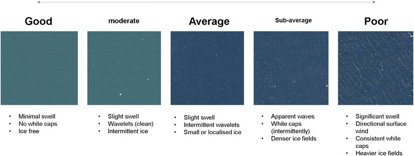
Figure 4. Linear scale of sea state showing that as sea state increases, the overall image quality decreases,
increasing the time required and the difficulty of the scanning process. Satellite image ©2020 Maxar
Technologies.
line are sighted, i.e., g(0) = 1, where g(x) is the probability of detecting an animal at distance x . For cetaceans,
the detection probability, g(x), is not assumed to be 163, as a consequence of their diving behaviours, and needs
to be accounted for if estimates are to be accurate. The detection probability is influenced by both species-specific
surface availability bias, and observer mediated perception bias, where animals that are available to be detected
are missed by the o bservers45. The effect of surface availability on g(0) can be accounted for by providing an
upward correction to estimates, whilst perception bias can be minimised through the use of experienced observ-
ers, training, and rotation to mitigate fatigue. No adjustment for g(x) were made to the ship survey data, as given
the highly conspicuous surface behaviour of humpback whales (> 95% of sightings) it is presumed unlikely that
the observers would have missed sighting a whale present on the transect line, particularly given the observer
bow-overlap. Furthermore, Johnston et al.16 demonstrate, using tag data, that for humpbacks in Gerlache Strait,
g(0) ≈ 1. In the absence of associated tagging data for the present study, we assume this is also the case for the
ship-based survey conducted here. Sightings data were analysed in the “Distance” p ackage64 in R v3.5.565. A
multiple covariate distance sampling (MCDS) framework was applied to groups of animals, assuming g(0) = 1.
Covariates tested included Beaufort sea state, visibility, and sightability. Visibility was measured on a linear scale
described by: Good (horizon clearly visible); Fair (no horizon, but visibility > 3 nautical miles); Poor (visibility < 3
nautical miles). Sightability was defined as: 0 (excellent); 1 (good); 2 (moderate); 3 (poor) based on conditions
required to reliably spot a minke whale. Perpendicular distance truncation at 5% was tested. Half-normal and
hazard rate keys were tested using no adjustment terms to fit the detection function. Model selection was based
on minimum Akaike’s information criterion (AIC) values66, and checking of the parameter estimates.
VHR image collection and analysis. Four WorldView-3 images were acquired totalling 866 k m2 (971
km2, including overlaps). Images 1 to 3 were taken on the 15 February 2018 and image 4 on 17 February 2018
(Fig. 3). Care was taken during analysis to prevent the introduction of double counts of features from overlap-
ping images, and images were scanned twice to prevent any FOIs from being erroneously omitted. Given the
ability to examine the images for extended periods, taking breaks regularly, and revisiting the entire region twice,
the likelihood of missing FOIs, if present in the image, was assumed to be nil. Animal movement into/out of
the study area was assumed to be no more likely than that encountered during a multi-day vessel survey, and
therefore double-counting was presumed not to influence the results. Images were scanned systematically by
eye using a 0.5 km by 0.5 km grid at a scale of 1:2,300 by experienced observers. Apparent sea state around the
FOI was also recorded during the imagery classification process using a linear scale between “ideal” and “poor”
indicating an increasing sea state (Fig. 4).
Image analysis followed that described in Cubaynes et al.31. Images were first loaded into ArcGIS v.10.4
(ESRI, 2017), and pan-sharpened using the ESRI algorithm,a process in which a higher resolution panchromatic
image (0.31 m) is used to enhance a coarser resolution multispectral image (1.24 m), yielding a high resolution
multispectral composite. In order to assess each whale-like feature in the image, candidate FOIs were identified
and classified using 13 distinct criteria taken from Cubaynes et al.31. These criteria are indicative of whale-like
characteristics that (1) stand out from the homogeneous environment, (2) are not easily replicated by background
conditions, and (3) closely align with the whale identification criteria implemented by ship-surveys. Criteria
were scored between 0 and 2, with 0 indicating that the criterion was not met, and the FOI did not conform to
a whale-like feature,scored as 1 if the FOI indicated partial conformity, typically characterised by blurred edges
and reduced clarity overall, and 2 if the FOI conformed to the criterion and thus indicated a whale-like feature.
Scores for each criteria (Cs ) were combined following:
Scientific Reports | (2020) 10:12985 | https://doi.org/10.1038/s41598-020-69887-y 8
Vol:.(1234567890)www.nature.com/scientificreports/
Deployment ID Time above 1 m (s) Time below 1 m (s) Total daylight duration of tag (s) Proportion of time at < 1 m
mn170218-31 16,186.2 20,824.0 37,010.2 0.44
mn170220-30 3,290.3 5,561.6 8,851.9 0.37
mn180227-40 11,330.8 12,016.0 23,346.8 0.49
mn180227-41 23,012.5 37,736.1 60,748.6 0.38
mn180227-43 27,609.2 36,505.8 64,115.0 0.43
mn180227-44 25,090.5 69,660.9 94,751.4 0.26
mn180227-45 212.4 685.2 897.6 0.24
mn180227-46 17,653.9 46,775.4 64,429.3 0.27
mn180227-47 309.8 619.5 929.3 0.33
mn180228-47 12,358.4 29,965.0 42,323.4 0.29
mn190203-22 24,306.4 71,692.5 95,998.9 0.25
mn190203-23 12,394.2 25,526.3 37,920.5 0.33
mn190205-27 19,229.8 45,189.7 64,419.5 0.30
mn190205-40 23,349.2 63,803.5 87,152.7 0.27
mn190212-27 6,658.6 18,529.3 25,187.9 0.26
mn190212-40 3,146.4 18,547.3 21,693.7 0.15
mn190215-40 7,653.3 35,539.3 43,192.6 0.18
mn190225-40 12,137.1 15,920.2 28,057.3 0.43
mn190225-44 1,448.0 992.8 2,440.8 0.59
mn190228-42 41,582.5 51,995.0 93,577.5 0.44
mn190228-44 27,466.5 11,853.8 39,320.3 0.70
Mean 15,068 29,521 44,589 0.34
SE 2,403 4,869 6,802 0.03
Table 3. Surface and dive times to the nearest second (s) of humpback whales (Megaptera novaeangliae)
tagged with digital time-depth devices in the Gerlache and surrounding bays during February 2017, 2018, and
2019. Mean of the proportion of time at < 1 m depth provided is weighted by tag duration.
Cs = ((ψ1 + ψ2 + ψ3 + ψ4 (·2)) + ψ5 + · · · ψ13 ) (1)
Weighting factors were assigned to Ψ1 through Ψ3, corresponding to visible fluke, fins and footprints in line
with Cubaynes et al.31. In this study we also weighted blow signs, Ψ4, by a factor of 2 in the effort to improve inter-
platform comparability, as these criteria are highly indicative of a whale and are commonly used when sighting
from a ship (i.e. if a visible blow is spotted, the sighting would be confirmed and recorded, and the weighting fac-
tor is designed to reflect this in the image survey). Cs for each whale was classified as either “definite”, “probable” or
“unclassified” FOIs based on the scoring system, where Cs > 9, "definite", if ≥ 7, "probable", and < 7, "unclassified”.
The initial scanning and classification of the imagery and FOIs was carried out by a single observer (O1). To
investigate the effect of inter-user variation, a randomly chosen subset of FOIs (n = 37, 20%) were reclassified by
three independent reviewers (R1-R3). We note, that as with at-sea marine mammal sightings, a level of previous
experience is likely to improve observations, and as such, experienced cetacean observers were used to review
the images. The average classification from these observers were then compared to those of the O1, to assess the
pattern of deviance between scores. If these were significantly different from O1, an adjustment to the original
FOIs scores was anticipated. The proportion of the subset of the FOIs identified as either “definite” or “probable”
was also estimated for O1, R1, R2 and R3.
Whale densities were estimated using the counts of “definite” and “probable” FOIs. These two criteria represent
identified features that resemble and are highly likely to be a whale. “Unclassified” FOIs typically represent
unusual surface disturbances, which can be scored according to some visibility criteria (e.g. the disturbances are
of a similar length, shape or width of a whale), but are not visually indicative of a whale-like feature when exam-
ined in detail. The total set of scored FOIs from O1 were fitted to a negative binomial distribution (Fig S3) using
the R package “fitdistplus”67. To obtain a measure of the classification uncertainty we assumed a binomial model,
and used this to calculate the standard error of the proportion ( p) to total FOIs (n) classified as either “definite”,
“probable” or “unclassified”, where standard error was calculated as p 1 − p /n.
Since satellite imagery acquisition is instantaneous, the combined total of “definite” and “probable” FOIs were
then corrected for availability bias. Availability bias was estimated based on an instantaneous viewing time. In
order estimate surface availability, suction cup archival tags with video and 3D accelerometery data from cus-
tomised Animal Tracking Solutions (https://www.CATS.is, as described in Cade et al.68, were deployed on 21
whales in February 2017, 2018 and 2019 in bays surrounding the study area, remaining attached and recording
data for an average of 20.08 ± 0.7 h. Depth data (collected at 10 Hz) was used to determine the mean daylight
surface time, Es and the mean dive time of each animal, Ed (Table 3). Using these data, Es , and Ed were calculated
from each of the individual whale IDs reported. Availability, â, weighted by tag duration, was estimated to be
0.34 (CV = 0.35), and density estimate, d̂ , was then corrected for availability bias, α̂, by d̂/α̂.
Scientific Reports | (2020) 10:12985 | https://doi.org/10.1038/s41598-020-69887-y 9
Vol.:(0123456789)www.nature.com/scientificreports/
Data availability
WorldView-3 images analysed herein were licensed from DigitalGlobe Inc., a subsidiary of Maxar Technologies
Inc., and are available to purchase from the archive at https://discover.digitalglobe.com/, using image ID num-
bers: 1040010038AFA900, 1040010039052600, 104001003757E500, and 104001003AC95B00. Ship survey data is
being held under an embargo period by the Brazilian Antarctic Program., please contact LDR. Bathymetry data
visualised is available freely from GEBCO_2014 30-arc second grid, version 20150318, https://www.gebco.net.
Received: 26 June 2019; Accepted: 7 July 2020
References
1. Buckland, S. T. et al. Introduction to distance sampling: estimating abundance of biological populations Vol. 335 (Oxford University
Press, Oxford, 2001).
2. 2Buckland, S. T., Rexstad, E. A., Marques, T. A. & Oedekoven, C. S. Distance sampling: methods and applications. (Springer, 2015).
3. Herr, H. et al. Horizontal niche partitioning of humpback and fin whales around the West Antarctic Peninsula: evidence from a
concurrent whale and krill survey. Polar Biol. 39, 799–818. https://doi.org/10.1007/s00300-016-1927-9 (2016).
4. Secchi, E. R. et al. Encounter rates and abundance of humpback whales (Megaptera novaeangliae) in Gerlache and Bransfield
Straits, Antarctic Peninsula. J. Cetac. Res. Manag. 3, 107–111 (2011).
5. 5Paxton, C. G., Hedley, S. L. & Bannister, J. L. Group IV humpback whales: their status from aerial and land-based surveys off
Western Australia, 2005. Journal Cetacean Research and Management, 223–234, https://iwcoffi ce.org/ (2011).
6. Branch, T. A. Abundance of Antarctic blue whales south of 60 S from three complete circumpolar sets of surveys. https: //hdl.handl
e.net/11427/17261 (2007).
7. Hammond, P. et al. Estimates of cetacean abundance in European Atlantic waters in summer 2016 from the SCANS-III aerial and
shipboard surveys. SCANS-III project report 1, 39 pp (2017).
8. 8Noad, M. J., Dunlop, R., Paton, D. & Cato, D. Absolute and relative abundance estimates of Australian east coast humpback whales
(Megaptera novaeangliae). J. Cetacean Res. Manage.(special issue 3) 243, 252 (2011).
9. Zerbini, A. N. et al. Winter distribution and abundance of humpback whales (Megaptera novaeangliae) off Northeastern Brazil.
J. Cetac. Res. Manag. 6, 101–107 (2004).
10. Barlow, J. & Forney, K. A. Abundance and population density of cetaceans in the California Current ecosystem. Fish. Bull. 105,
509–526, https://aquaticcommons.org/id/eprint/8866 (2007).
11. Kaschner, K., Quick, N. J., Jewell, R., Williams, R. & Harris, C. M. Global coverage of cetacean line-transect surveys: status quo,
data gaps and future challenges. PLoS ONE 7, e44075. https://doi.org/10.1371/journal.pone.0044075 (2012).
12. Branch, T. A. Humpback whale abundance south of 60 S from three complete circumpolar sets of surveys. J. Cetac. Res. Manag. 3,
53–69 (2011).
13. Branch, T. & Butterworth, D. Southern Hemisphere minke whales: standardised abundance estimates from the 1978/79 to 1997/98
IDCR-SOWER surveys. J. Cetac. Res. Manag. 3, 143–174 (2001).
14. Griffiths, H. J. Antarctic marine biodiversity–what do we know about the distribution of life in the Southern Ocean?. PLoS ONE
5, e11683. https://doi.org/10.1371/journal.pone.0011683 (2010).
15. Secchi, E. R. et al. Encounter rates of whales around the Antarctic Peninsula with special reference to humpback whales, Megaptera
Novaeangliae, in the Gerlache strait: 1997/98 to 1999/2000. Memoirs Queensl. Museum 47, 571–578 (2001).
16. Johnston, D., Friedlaender, A., Read, A. & Nowacek, D. Initial density estimates of humpback whales Megaptera novaeangliae in the
inshore waters of the western Antarctic Peninsula during the late autumn. Endanger. Spec. Res. 18, 63–71. https://doi.org/10.3354/
esr00395 (2012).
17. Dalla Rosa, L., Secchi, E. R., Maia, Y. G., Zerbini, A. N. & Heide-Jørgensen, M. P. Movements of satellite-monitored humpback
whales on their feeding ground along the Antarctic Peninsula. Polar Biol. 31, 771–781. https://doi.org/10.1007/s00300 -008-0415-2
(2008).
18. Viquerat, S. & Herr, H. Mid-summer abundance estimates of fin whales Balaenoptera physalus around the South Orkney Islands
and Elephant Island. Endanger. Spec. Res. 32, 515–524. https://doi.org/10.3354/esr00832 (2017).
19. Reilly, S. et al. Biomass and energy transfer to baleen whales in the South Atlantic sector of the Southern Ocean. Deep Sea Res.
Part II 51, 1397–1409. https://doi.org/10.1016/s0967-0645(04)00087-6 (2004).
20. Williams, R. et al. Counting whales in a challenging, changing environment. Sci. Rep. 4, 4170. https://doi.org/10.1038/srep04170
(2014).
21. Nicol, S., Pauly, T., Bindoff, N. & Strutton, P. “BROKE” a biological/oceanographic survey off the coast of East Antarctica (80–150°
E) carried out in January–March 1996. Deep Sea Res. Part II 47, 2281–2297. https: //doi.org/10.1016/S0967- 0645(00)00026- 6 (2000).
22. Nicol, S., Meiners, K. & Raymond, B. BROKE-West, a large ecosystem survey of the South West Indian Ocean sector of the South-
ern Ocean, 30E–80E (CCAMLR Division 5842). Deep Sea Res Part II Top. Stud. Oceanogr. 57, 693–700. https://doi.org/10.1016/j.
dsr2.2009.11.002 (2010).
23. Leaper, R. & Miller, C. Management of Antarctic baleen whales amid past exploitation, current threats and complex marine eco-
systems. Antarct. Sci. 23, 503–529. https://doi.org/10.1017/s0954102011000708 (2011).
24. Angliss, R. P. et al. Comparing manned to unmanned aerial surveys for cetacean monitoring in the Arctic: methods and operational
results. J. Unman. Vehicle Syst. 6, 109–127. https://doi.org/10.1139/juvs-2018-0001 (2018).
25. Ferguson, M. et al. Performance of manned and unmanned aerial surveys to collect visual data and imagery for estimating arctic
cetacean density and associated uncertainty. J. Unman. Vehicle Syst. https://doi.org/10.1139/juvs-2018-0002 (2018).
26. Hodgson, A., Kelly, N. & Peel, D. Unmanned aerial vehicles (UAVs) for surveying marine fauna: a dugong case study. PLoS ONE
8, e79556. https://doi.org/10.1371/journal.pone.0079556 (2013).
27. Buckland, S. T. et al. Aerial surveys of seabirds: the advent of digital methods. J. Appl. Ecol. 49, 960–967. https://doi.org/10.111
1/j.1365-2664.2012.02150.x (2012).
28. Fiori, L., Doshi, A., Martinez, E., Orams, M. B. & Bollard-Breen, B. The use of unmanned aerial systems in marine mammal
research. Remote Sens. 9, 543. https://doi.org/10.3390/rs9060543 (2017).
29. Abileah, R. Marine Mammal Census Using Space Satellite Imagery. U.S. Navy J. Underw. Acosist. 52, 709–724 (2002).
30. Fretwell, P. T., Staniland, I. J. & Forcada, J. Whales from space: counting southern right whales by satellite. PLoS ONE 9, e88655.
https://doi.org/10.1371/journal.pone.0088655 (2014).
31. Cubaynes, H. C., Fretwell, P. T., Bamford, C., Gerrish, L. & Jackson, J. A. Whales from space: four mysticete species described using
new VHR satellite imagery. Mar. Mammal Sci. 35, 466–491. https://doi.org/10.1111/mms.12544 (2019).
32. Platonov, N. G., Mordvintsev, I. N. & Rozhnov, V. V. The possibility of using high resolution satellite images for detection of marine
mammals. Biol. Bull. 40, 197–205. https://doi.org/10.1134/s1062359013020106 (2013).
33. Fretwell, P. T., Scofield, P. & Phillips, R. A. Using super-high resolution satellite imagery to census threatened albatrosses. Ibis 159,
481–490. https://doi.org/10.1111/ibi.12482 (2017).
Scientific Reports | (2020) 10:12985 | https://doi.org/10.1038/s41598-020-69887-y 10
Vol:.(1234567890)www.nature.com/scientificreports/
34. Fretwell, P. T. et al. An emperor penguin population estimate: the first global, synoptic survey of a species from space. PLoS ONE
7, e33751. https://doi.org/10.1371/journal.pone.0033751 (2012).
35. LaRue, M. A. et al. Satellite imagery can be used to detect variation in abundance of Weddell seals (Leptonychotes weddellii) in
Erebus Bay Antarctica. Polar Biol. 34, 1727–1737. https://doi.org/10.1007/s00300-011-1023-0 (2011).
36. Stapleton, S. et al. Polar bears from space: assessing satellite imagery as a tool to track Arctic wildlife. PLoS ONE 9, e101513. https
://doi.org/10.1371/journal.pone.0101513 (2014).
37. Larue, M. A. & Knight, J. Applications of very high-resolution imagery in the study and conservation of large predators in the
Southern Ocean. Conserv. Biol. 28, 1731–1735. https://doi.org/10.1111/cobi.12367 (2014).
38. LaRue, M. A. et al. A method for estimating colony sizes of Adélie penguins using remote sensing imagery. Polar Biol. 37, 507–517.
https://doi.org/10.1007/s00300-014-1451-8 (2014).
39. Lynch, H. J. & LaRue, M. A. First global census of the Adélie Penguin. Auk 131, 457–466. https://doi.org/10.1642/auk-14-31.1
(2014).
40. McMahon, C. R. et al. Satellites, the all-seeing eyes in the sky: counting elephant seals from space. PLoS ONE 9, e92613. https://
doi.org/10.1371/journal.pone.0092613 (2014).
41. LaRue, M. A., Stapleton, S. & Anderson, M. Feasibility of using high-resolution satellite imagery to assess vertebrate wildlife
populations. Conserv. Biol. 31, 213–220. https://doi.org/10.1111/cobi.12809 (2017).
42. LaRue, M. A. & Stapleton, S. Estimating the abundance of polar bears on Wrangel Island during late summer using high-resolution
satellite imagery: a pilot study. Polar Biol. 41, 2621–2626. https://doi.org/10.1007/s00300-018-2384-4 (2018).
43. Weinstein, B. G. & Friedlaender, A. S. Dynamic foraging of a top predator in a seasonal polar marine environment. Oecologia 185,
427–435. https://doi.org/10.1007/s00442-017-3949-6 (2017).
44. Marques, F. & Buckland, S. Covariate models for the detection function. Adv. Dist. Sampling, 31–47 (2004).
45. Marsh, H. & Sinclair, D. F. Correcting for visibility bias in strip transect aerial surveys of aquatic fauna. J. Wildl. Manag. 1,
1017–1024. https://doi.org/10.2307/3809604 (1989).
46. Durban, J. W. & Pitman, R. L. Antarctic killer whales make rapid, round-trip movements to subtropical waters: evidence for physi-
ological maintenance migrations?. Biol. Lett. 8, 274–277. https://doi.org/10.1098/rsbl.2011.0875 (2012).
47. Pitman, R. L. & Durban, J. W. Cooperative hunting behavior, prey selectivity and prey handling by pack ice killer whales (Orcinus
orca), type B Antarctic Peninsula waters. Mar. Mammal Sci. 28, 16–36. https://doi.org/10.1111/j.1748-7692.2010.00453.x (2012).
48. Pitman, R. L. & Durban, J. W. Killer whale predation on penguins in Antarctica. Polar Biol. 33, 1589–1594. https: //doi.org/10.1007/
s00300-010-0853-5 (2010).
49. Laake, J. L., Calambokidis, J., Osmek, S. D. & Rugh, D. J. Probability of detecting harbor porpoise from aerial surveys: estimating
g(0). J. Wildl. Manag. 61, 63–75. https://doi.org/10.2307/3802415 (1997).
50. Watkins, W. A. et al. Sperm whale dives tracked by radio tag telemetry. Mar. Mammal Sci. 18, 55–68. https : //doi.
org/10.1111/j.1748-7692.2002.tb01018.x (2002).
51. Cubaynes, H. C. et al. Spectral reflectance of whale skin above the sea surface: a proposed measurement protocol. Remote Sens.
Ecol. Conserv. https://doi.org/10.1002/rse2.155 (2020).
52. Hodgson, A., Peel, D. & Kelly, N. Unmanned aerial vehicles for surveying marine fauna: assessing detection probability. Ecol. Appl.
27, 1253–1267. https://doi.org/10.1002/eap.1519 (2017).
53. Heide-Jørgensen, M., Witting, L., Laidre, K., Hansen, R. & Rasmussen, M. Fully corrected estimates of common minke whale
abundance in West Greenland in 2007. J. Cetac. Res. Manag. 11, 75–82 (2010).
54. Hiby, L. & Lovell, P. Using aircraft in tandem formation to estimate abundance of harbour porpoise. Biometrics 1, 1280–1289. https
://doi.org/10.2307/2533658 (1998).
55. Borowicz, A. et al. Aerial-trained deep learning networks for surveying cetaceans from satellite imagery. PLoS ONE 14, e0212532.
https://doi.org/10.1371/journal.pone.0212532 (2019).
56. Guirado, E., Tabik, S., Rivas, M. L., Alcaraz-Segura, D. & Herrera, F. Whale counting in satellite and aerial images with deep learn-
ing. Sci. Rep. 9, 14259. https://doi.org/10.1038/s41598-019-50795-9 (2019).
57. LaRue, M. A. et al. Engaging ‘the crowd’ in remote sensing to learn about habitat affinity of the Weddell seal in Antarctica. Remote
Sens. Ecol. Conserv. 6, 70–78. https://doi.org/10.1002/rse2.124 (2019).
58. Nicol, S., Worby, A. & Leaper, R. Changes in the Antarctic sea ice ecosystem: potential effects on krill and baleen whales. Mar.
Freshw. Res. 59, 361–382. https://doi.org/10.1071/MF07161 (2008).
59. Xavier, J. C. et al. Future challenges in Southern Ocean ecology research. Front. Mar. Sci. 3, 94. https://doi.org/10.3389/fmars
.2016.00094(2016).
60. Thiele, D. et al. Seasonal variability in whale encounters in the Western Antarctic Peninsula. Deep Sea Res. Part II 51, 2311–2325.
https://doi.org/10.1016/j.dsr2.2004.07.007 (2004).
61. Lerczak, J. A. & Hobbs, R. C. Calculating sighting distances from angular readings during shipboard, aerial, and shore-based
marine mammal surveys. Mar. Mammal Sci. 14, 590–598. https://doi.org/10.1111/j.1748-7692.1998.tb00745.x (1998).
62. Logger Software. International fund for animal welfare, PO Box 193, 411 Main Stree, Yarmouth Port, MA 02675, USA (2010).
63. Barlow, J. Inferring trackline detection probabilities, g (0), for cetaceans from apparent densities in different survey conditions.
Mar. Mammal Sci. 31, 923–943. https://doi.org/10.1111/mms.12205 (2015).
64. Miller, D. L. Package ‘Distance’. (2019).
65. R: A language and environment for statistical computing v. v3.5.3 (R Foundation for Statistical Computing, Vienna, Austria, 2019).
66. Akaike, H. in A new look at the statistical model identification: Selected Papers of Hirotugu Akaike 215–222 (Springer, 1974).
67. Delignette-Muller, M. L. & Dutang, C. fitdistrplus: An R package for fitting distributions. J. Stat. Softw. 64, 1–34 (2015).
68. Cade, D. E., Friedlaender, A. S., Calambokidis, J. & Goldbogen, J. A. Kinematic diversity in rorqual whale feeding mechanisms.
Curr. Biol. 26, 2617–2624. https://doi.org/10.1016/j.cub.2016.07.037 (2016).
Acknowledgements
This work was funded by WWF grant GB107301 “Counting Southern Ocean Giants” and further supported by
Natural Environmental Research Council Grant number NE/L002531/1. The ship-based survey was conducted
within the activities of research project Baleias, of the Brazilian Antarctic Program, financed by the National
Council for Scientific and Technological Development (CNPq grant number 408096/2013-6) under the Brazilian
Ministry of Science, Technology, Innovations and Communications—MCTIC. CNPq also provided a research
fellowship to LDR (PQ 309258/2016-2). We thank all crew members of the polar vessel Almirante Maximiano.
J.H. Prado, F.R. Castro, M. Bassoi and E. Seyboth helped with data collection. ASF is supported by National Sci-
ence Foundation Office of Polar Programs award number 1643877. Surface availability data were collected under
National Marine Fisheries Service permit numbers 14809, 23095, ACA 2015-011, and UCSC IACUC Friea1706.
The authors would also like to thank DigitalGlobe Inc., a subsidiary of Maxar Technologies Inc., from whom
the images analysed here are licensed, for their assistance and patience in coordinating image acquisition with
a weather-dependent ship survey.
Scientific Reports | (2020) 10:12985 | https://doi.org/10.1038/s41598-020-69887-y 11
Vol.:(0123456789)You can also read