Observations of iodine monoxide over three summers at the Indian Antarctic bases of Bharati and Maitri
←
→
Page content transcription
If your browser does not render page correctly, please read the page content below
Atmos. Chem. Phys., 21, 11829–11842, 2021
https://doi.org/10.5194/acp-21-11829-2021
© Author(s) 2021. This work is distributed under
the Creative Commons Attribution 4.0 License.

Observations of iodine monoxide over three summers
at the Indian Antarctic bases of Bharati and Maitri
Anoop S. Mahajan1 , Mriganka S. Biswas1,2 , Steffen Beirle3 , Thomas Wagner3 , Anja Schönhardt4 , Nuria Benavent5 ,
and Alfonso Saiz-Lopez5
1 Centre  for Climate Change Research, Indian Institute of Tropical Meteorology,
Ministry of Earth Sciences, Pune, 411008, India
2 Atmospheric and Space Sciences, Savitribai Phule Pune University, Pune, 411008, India
3 Satellitenfernerkundung, Max-Planck-Institut für Chemie (MPI-C), 55128 Mainz, Germany
4 Department of Physics and Electrical Engineering, Institute of Environmental Physics,

University of Bremen, 330440 Bremen, Germany
5 Department of Atmospheric Chemistry and Climate, Institute of Physical Chemistry Rocasolano,

CSIC, 28006 Madrid, Spain

Correspondence: Anoop S. Mahajan (anoop@tropmet.res.in)

Received: 25 September 2020 – Discussion started: 20 November 2020
Revised: 28 April 2021 – Accepted: 30 April 2021 – Published: 9 August 2021

Abstract. Iodine plays a vital role in oxidation chemistry          dataset to validate models estimating the impacts of iodine
over Antarctica, with past observations showing highly el-          chemistry.
evated levels of iodine oxide (IO) leading to severe depletion
of boundary layer ozone in West Antarctica. Here, we present
MAX-DOAS-based (multi-axis differential absorption spec-
troscopy) observations of IO over three summers (2015–              1   Introduction
2017) at the Indian Antarctic bases of Bharati and Maitri.
IO was observed during all the campaigns with mixing ra-            Reactive halogen species (RHS) have been shown to play
tios below 2 pptv (parts per trillion by volume) for the three      a critical role in causing ozone depletion events in the po-
summers, which are lower than the peak levels observed in           lar boundary layer (BL) (Barrie et al., 1988; Bottenheim et
West Antarctica. This suggests that sources in West Antarc-         al., 1986; Kreher et al., 1997; Oltmans and Komhyr, 1986)
tica are different or stronger than sources of iodine com-          and could contribute to new particle formation in this re-
pounds in East Antarctica, the nature of which is still uncer-      mote environment (Allan et al., 2015; Atkinson et al., 2012;
tain. Vertical profiles estimated using a profile retrieval algo-   O’Dowd et al., 2004). Observations of RHS have been made
rithm showed decreasing gradients with a peak in the lower          in the Antarctic BL for almost two decades. Early observa-
boundary layer. The ground-based instrument retrieved ver-          tions focused on bromine oxide (BrO), the presence of which
tical column densities (VCDs) were approximately a factor           was observed in the Antarctic using ground-based instru-
of 3 to 5 higher than the VCDs reported using satellite-based       ments (Kreher et al., 1997) and via satellites (Hollwedel et
instruments, which is most likely related to the sensitivi-         al., 2004). The presence of iodine oxide (IO) in the Antarctic
ties of the measurement techniques. Air mass back-trajectory        atmosphere was also confirmed through integrated column
analysis failed to highlight a source region, with most of the      measurements from the ground (Frieß et al., 2001). Later,
air masses coming from coastal or continental regions. This         year-long ground-based observations of RHS made at Halley
study highlights the variation in iodine chemistry in differ-       Bay showed the critical role that bromine and iodine com-
ent regions in Antarctica and the importance of a long-term         pounds play in regulating the oxidizing capacity, causing
                                                                    ozone depletion and new particle formation in the Antarc-
                                                                    tic BL (Saiz-Lopez et al., 2007a). These ground-based ob-

Published by Copernicus Publications on behalf of the European Geosciences Union.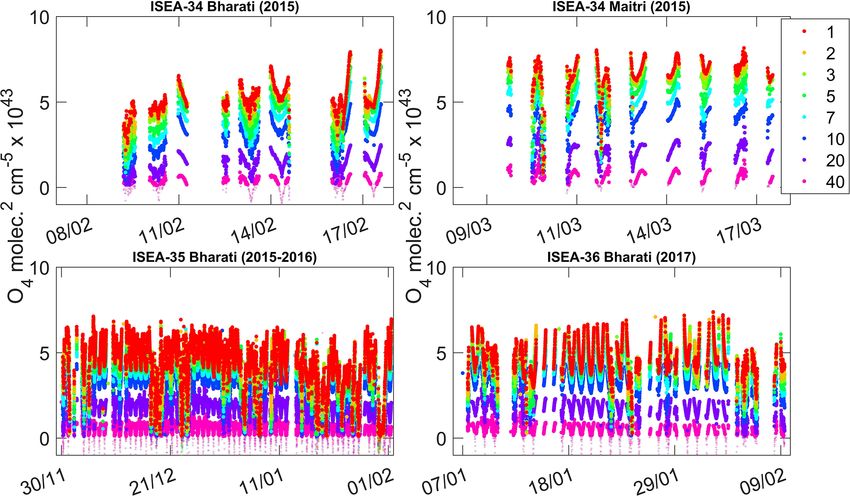
11830          A. S. Mahajan et al.: Observations of iodine monoxide over three summers at the Indian Antarctic bases

servations show that both IO and BrO are present at ele-           ment (∼ 7×10¹² molec. cm−2 for a single measurement) and
vated concentrations (from 1 to as high as 20 pptv) in certain     are therefore subject to uncertainties. The study by Frieß et
parts of the Antarctic BL and show a significant seasonal          al. (2010) suggested a strong source within the snowpack,
variation peaking in the spring, with elevated concentra-          which hints at active recycling and re-emission of IO aiding
tions observed through the summer (Saiz-Lopez et al., 2008).       the long transport inland. However, questions remain about
Satellite-based observations of both IO and BrO reported a         why such a source would function only in parts of the con-
similar annual cycle, although with large geographical dif-        tinent and why the primary source is different from the Arc-
ferences (Hollwedel et al., 2004; Richter et al., 2002; Saiz-      tic, where much lower peak concentrations are sporadically
Lopez et al., 2007b; Schönhardt et al., 2008, 2012; Theys et       observed (Mahajan et al., 2010; Saiz-Lopez and Blaszczak-
al., 2011; Wagner et al., 2001). These satellite observations      boxe, 2016). To further understand the sources of iodine in
have been validated by ground-based observations, although         the polar environment, understanding the geographical dis-
most of them have hitherto focused on the area around the          tribution is critical. Satellite observations play a useful role
Weddell Sea (Atkinson et al., 2012; Buys et al., 2013; Frieß       for this, although validation of the satellite observations us-
et al., 2001, 2010; Saiz-Lopez et al., 2007a, 2008). Previ-        ing ground-based instruments is necessary to ascertain their
ous studies show that similar levels of BrO have been ob-          accuracy when observing IO in the Antarctic troposphere.
served between the Arctic and Antarctic, while much lower             Questions also remain about the vertical profiles of iodine
levels of atmospheric iodine have been reported in the Arctic      compounds within and above the Antarctic boundary layer.
compared to the Antarctic (Hönninger et al., 2004; Raso et         Modeling-based studies using the one-dimensional Tropo-
al., 2017; Schönhardt et al., 2008; Tuckermann et al., 1997).      spheric Halogen Chemistry MOdel (THAMO) have sug-
The satellite observations also show a difference in the geo-      gested a strong gradient in IO from the surface to the edge
graphical distribution of IO over Antarctica, with the Wed-        of the boundary layer (Saiz-Lopez et al., 2008). Only once
dell sea being an iodine hotspot, the reasons for which are        in the past have vertical profiles of IO been measured in
still not completely clear (Saiz-Lopez and Blaszczak-boxe,         Antarctica using the multi-axis differential optical absorp-
2016). Ground-based observations have also been made at            tion spectroscopy (MAX-DOAS) instrument. These mea-
McMurdo Sound, near the Ross Sea, where lower concen-              surements were made at McMurdo Sound in East Antarctica
trations of IO were observed (Hay, 2010). Additional ob-           (Hay, 2010). Observations over 2 “golden days” in 2006 and
servations over the 2011–2012 summer were made at Du-              2007 show surface concentrations of about 1 pptv, decreas-
mont d’Urville Station using a cavity-enhanced absorption-         ing to ∼ 0.2 pptv at about 200 m, before reaching a second
spectroscopy-based instrument and showed a maximum of              maximum of 0.6 pptv at ∼ 700 m. The detection limit was
0.15 pptv of IO (Grilli et al., 2013). However, observations       estimated to be about ∼ 0.5 pptv. However, models did not
of IO have not been reported in the Indian Ocean sector of         reproduce this measured IO vertical profile shape, and there
the Antarctic peninsula to date (Saiz-Lopez et al., 2012; Saiz-    are also large uncertainties associated with the a priori pro-
Lopez and von Glasow, 2012).                                       file (Hay, 2010). In most models, the assumption is that the
   Ground-based observations at Halley Bay and in the Wed-         source of iodine compounds is from the snowpack, with pho-
dell Sea suggest that the main source of iodine compounds is       tochemistry in the atmosphere resulting in a steady decrease
the sea ice region based on observations of iodocarbons and        with altitude. However, considerable challenges remain in
back trajectory analysis (Atkinson et al., 2012; Saiz-Lopez        reproducing the surface variation and vertical gradients in
et al., 2007a). Other studies have also measured iodocarbons       addition to the geographical distribution (Fernandez et al.,
in Antarctica, although their levels are too low to explain the    2019). More recent modeling studies combined with aircraft
high levels of IO observed in the Weddell Sea region (Car-         observations suggest that the gradient is not very sharp at all
penter et al., 2007; Fogelqvist and Tanhua, 1995; Reifen-          the latitudes, with a significant free tropospheric and strato-
häuser and Heumann, 1992). The exact process is still not          spheric contribution to the total column of IO (Koenig et al.,
known, although a mechanism for biologically induced io-           2020; Saiz-Lopez et al., 2015b), although such observations
dine emissions from sea ice has been suggested based on the        have still not been done in the Antarctic. One of the main
idea that micro-algae (Garrison and Buck, 1989) are the pri-       reasons for the uncertainties in models is the lack of con-
mary source of iodine emissions in this environment (Saiz-         sistent measurements of vertical gradients across the world,
Lopez et al., 2015a), with halogen compounds then mov-             especially in the polar regions, to validate these model simu-
ing up brine channels in the sea ice to finally get released       lations.
into the atmosphere. There are further questions regarding            Considering the uncertainties in the satellite observations
the propagation of reactive iodine chemistry across the con-       and questions regarding the sources and vertical and geo-
tinent because satellite observations show the presence of IO      graphical distribution of IO, further observations are neces-
deep within the Antarctic continent, even as far as the South      sary. Here we present observations made at two new loca-
Pole (Saiz-Lopez et al., 2007b; Schönhardt et al., 2008).          tions in Antarctica over three summers and compare them
However, although enhanced, the observed IO column den-            with the satellite-based retrievals and past observations.
sities are close to the detection limit of the satellite instru-

Atmos. Chem. Phys., 21, 11829–11842, 2021                                          https://doi.org/10.5194/acp-21-11829-2021
A. S. Mahajan et al.: Observations of iodine monoxide over three summers at the Indian Antarctic bases                             11831

                                                                          Bharati station and was approximately 56 m above sea level.
                                                                          The scanner unit was mounted on the wall of the hut and
                                                                          had a clear line of sight to the horizon, pointing −23.2◦ with
                                                                          respect to north and overlooking the open ocean. The coast-
                                                                          line is within 500 m of the hut, but it becomes ice free from
                                                                          mid-January to late March. Depending on the sea ice condi-
                                                                          tions, the open ocean is within 8–10 km north from the end
                                                                          of November.
                                                                             The MAX-DOAS instrument (EnviMeS) makes use of
                                                                          scattered sunlight along different elevation angles and by the
                                                                          combination of several lines of sight including the zenith.
                                                                          The concentration of an absorber in the boundary layer can
                                                                          be obtained either in a first approximation by a simple geo-
                                                                          metric approach or by simulating the light path with a radia-
                                                                          tive transfer model also taking into account multiple scatter-
                                                                          ing effects and the correct treatment of the aerosol loading
                                                                          in the atmosphere (Hönninger et al., 2004; Platt and Stutz,
Figure 1. Map showing the location of the two Indian Antarctic sta-       2008; Wagner et al., 2004). The instrument consists of an
tions, Maitri and Bharati, where observations of IO were performed        indoor unit housing a spectrometer with a spectral resolution
during this study (blue dots). Previous locations that have reported      of 0.7 nm (UV: 301.20–463.69) which is connected to an out-
observations of IO (Frieß et al., 2001; Grilli et al., 2013; Hay, 2010;   door unit containing a scanning telescope. Discrete elevation
Saiz-Lopez et al., 2007a) are also marked on the map (red dots).          angles (1, 2, 3, 5, 7, 10, 20, 40, and 90◦ ) were recorded for a
                                                                          total exposure time of 1 min each during all four campaigns.
                                                                          The spectra were recalibrated before analysis using mercury
2   Methodology                                                           emission lines recorded at the end of each day. For DOAS
                                                                          retrieval, the QDOAS 3.2 software was used (Fayt and Van
Figure 1 shows the location of the two Indian Antarctic                   Roozendael, 2013). For estimation of the O4 differential slant
stations, Maitri (70.77◦ S, 11.73◦ E) and Bharati (69.41◦ S,              column densities (DSCDs), the cross-sections of O4 (Thal-
76.19◦ E). The other stations where observations of IO have               man and Volkamer, 2013) at 293 K; NO2 (Vandaele et al.,
been reported in the past are also marked on the map. Obser-              1998) at 220 and 298 K (220 K orthogonalized to 294 K); O3
vations of IO and the oxygen dimer (O4 ) were made using                  (Bogumil et al., 2003) at 223 and 243 K (orthogonalized to
the multi-axis differential optical absorption spectroscopy               O3 at 243 K); HCHO (Meller and Moortgat, 2000) at 298 K;
(MAX-DOAS) technique over three summers: February–                        and HONO (Stutz et al., 2000) at 296 K were used in the 351–
March 2015 as part of the 34th Indian Scientific Expedition               390 nm window. The cross-sections used for IO retrieval in
to Antarctica (ISEA-34), November 2015–February 2016 as                   the 417–440 nm spectral window were IO (Gómez Martín et
a part of ISEA-35, and January–February 2017 as a part of                 al., 2005), NO2 at both 220 and 298 K (Vandaele et al., 1998),
ISEA-36.                                                                  H2 O (Rothman et al., 2013), O4 (Thalman and Volkamer,
   Observations at Maitri station were made over a short span             2013), and O3 (Bogumil et al., 2003). In addition to these
of 9 d (9–17 March 2015) and only during ISEA-34. The re-                 cross-sections a ring spectrum (Chance and Spurr, 1997), a
search station is in the ice-free rocky area on the Schirmacher           second ring spectrum following Wagner et al. (2009), and
Oasis. The MAX-DOAS instrument was installed in a sum-                    the third-order polynomial were used for both windows. The
mertime residential container ∼ 150 m north of the station                zenith spectrum from each scan was used as a reference to
and about 120 m above sea level during ISEA-34. The scan-                 remove the contribution from possible free tropospheric or
ner unit was mounted on top of the container with a clear line            stratospheric absorption. An example of a DOAS fit for O4
of sight to the horizon. The scanner pointed ∼ 60.0◦ with                 and IO are given in Fig. S1 in the Supplement. Surface mix-
respect to magnetic north. The spectrometer unit was kept                 ing ratios and the total vertical column densities (VCDs)
inside the container, which was temperature controlled. The               were retrieved from the MAX-DOAS DSCDs of IO and O4
open ocean is 125 km north of Maitri.                                     by employing the Mainz profile algorithm (MAPA) (Beirle et
   Observations at Bharati station were made for 10 d (9–                 al., 2018). Only observations with solar zenith angles (SZAs)
18 February 2015) during ISEA-34, for 63 d (30 Novem-                     less than 75◦ were used for the profile retrievals due to the
ber 2015–1 February 2016) during ISEA-35, and for 35 d                    large path lengths through the stratosphere for large SZAs.
(5 January–11 February 2017) during ISEA-36. The station                  This algorithm uses a two-step approach to determine the
is located between the Thala Fjord and Quilty Bay, east of                trace gas vertical profiles. In the first step, the aerosol pro-
the Stornes Peninsula. The MAX-DOAS instrument was in-                    files are retrieved using the measured O4 DSCDs. A Monte
stalled in a hut on top of a ridge around 200 m southwest of              Carlo approach is utilized to identify the best ensemble of

https://doi.org/10.5194/acp-21-11829-2021                                               Atmos. Chem. Phys., 21, 11829–11842, 2021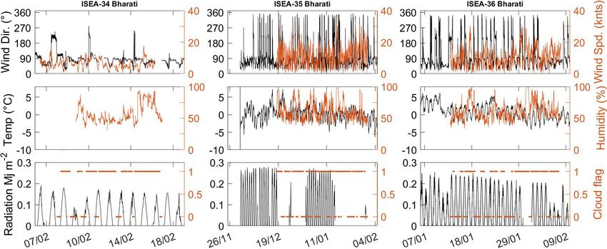
11832           A. S. Mahajan et al.: Observations of iodine monoxide over three summers at the Indian Antarctic bases

Figure 2. The 5 d back-trajectories arriving at the two stations on the days that the measurements of IO were conducted as a part of the 34th,
35th, and 36th ISEA expeditions are shown. The back-trajectories were calculated using the HYbrid Single-Particle Lagrangian Integrated
Trajectory (HYSPLIT) model, arriving every hour (Draxler and Rolph, 2003).

the forward model parameters – column parameter (c) (VCD                    We also make use of the IO vertical column densities
for trace gases and aerosol optical depth for aerosol), height           retrieved using the SCanning Imaging Absorption spec-
parameter (h), and shape parameter (s) – which fit the mea-              troMeter for Atmospheric CartograpHY (SCIAMACHY), a
sured O4 DSCDs for the sequence of elevation angles. In the              UV–vis–NIR (ultraviolet–visible–near-infrared) spectrome-
second step, the aerosol profiles retrieved from the O4 inver-           ter on board the ENVISAT satellite (Burrows et al., 1995).
sion are used as an input to retrieve similar model parameters           Observations from SCIAMACHY stopped due to instrumen-
(c, h, and s) for IO. The state of the atmosphere was calcu-             tal problems in April 2012. Here we make use of the mean
lated using the pressure and temperature profiles observed by            from 2004 to 2011 to look at the geographical distribution
the in situ radiosondes, which were launched once a week at              and compare it with the ground-based observations made
both stations. An Ångstrom exponent of 1 was used for the                during the study period. Further details about the IO retrieval
difference in the retrieval wavelengths as per observations              algorithm and the SCIAMACHY instrumental setup can be
made at Bharati in the past (Prakash Chaubey et al., 2011).              found elsewhere (Schönhardt et al., 2008, 2012).
Within MAPA, the differential air mass factors (AMFs) are
calculated offline with the radiative transfer model McArtim
(Deutschmann et al., 2011) for fixed nodes for each parame-              3     Results and discussion
ter and stored as a lookup table (LUT) for quick analysis. To
assess the quality of the retrievals, MAPA provides “valid”,             3.1    Meteorological parameters
“warning”, or “error” flags for each measurement sequence,
which are calculated based on pre-defined thresholds for var-            Figure 2 shows the 5 d back-trajectories arriving every hour
ious fit parameters. For further details about MAPA, please              at the two stations at a height of 10 m on the days that the
refer to the description paper by Beirle et al. (2018). Addi-            DOAS measurements were conducted as a part of the three
tionally, MAPA provides the option to use a scaling factor               ISEA expeditions. The back-trajectories were calculated
for significant mismatch between the modeled and measured                with the HYbrid Single-Particle Lagrangian Integrated Tra-
O4 DSCDs, which has been shown to be close to 0.8 in the                 jectory (HYSPLIT) model using the EDAS-40 km database
past (Wagner et al., 2019). For this study, the scaling factor           (Draxler and Rolph, 2003). The trajectories show that the air
ranged between 0.75 and 0.9. Therefore, a scaling factor of              masses sampled throughout the three expeditions were from
0.8 was applied for all the campaigns.                                   either a remote oceanic region, coastal Antarctica, or the con-
                                                                         tinental shelf. In general, most of the trajectories show that

Atmos. Chem. Phys., 21, 11829–11842, 2021                                                  https://doi.org/10.5194/acp-21-11829-2021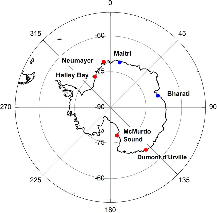
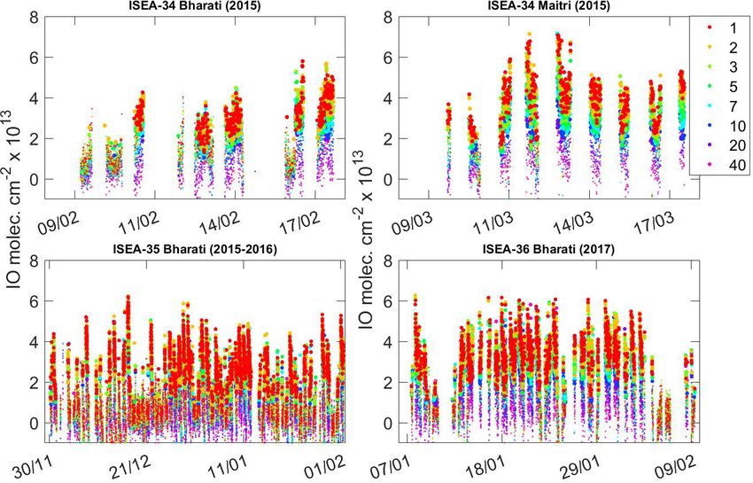
A. S. Mahajan et al.: Observations of iodine monoxide over three summers at the Indian Antarctic bases                         11833

Figure 3. Observations of different meteorological parameters that were measured during the various summer campaigns are shown here.
The top panels show the wind direction and speed, the middle panels show the temperature and humidity, and the bottom panels show the
radiation and cloudiness (1 is defined as 30 % cloudy skies and above). Observations of these parameters were not made during the 34th
ISEA at Maitri, and the gaps indicate instrumental or observational issues. The data had a time resolution of 5 min.

the air masses had traveled hundreds of kilometers over the          dex calculation. Meteorological data were unfortunately not
last 5 d. For the local meteorological conditions, Fig. 3 (top       available at Maitri station.
panels) shows the wind direction at Bharati station. Most of
the time, the wind was from the ocean, with the winds com-           3.2   Differential slant column densities (DSCDs)
ing from the northwest sector and a few instances of northern
and northeastern winds (although during ISEA-34 the winds            Figure 4 shows the observed O4 DSCDs at different eleva-
were mostly from east to northeast). This was during all three       tion angles for all the campaigns. O4 DSCDs were found to
expeditions at Bharati station. The wind speed was mostly            be higher at lower elevation angles, as expected, which is
below 20 kn (∼ 10 m s−1 ) for all the campaigns, although            because the O4 concentration is proportional to the square
periods of high winds were observed during ISEA-35 and               of the oxygen pressure and thus increases towards the sur-
ISEA-36, which were of a longer duration than ISEA-34. The           face. This also suggests that the aerosol loading was low
temperature at the station hovered between −5 and +5 ◦ C             in the atmosphere. Photons travel longer paths at lower el-
throughout the summer period, with higher values closer to           evation angles and interact more with tropospheric absorb-
noon (Fig. 3, middle panels). The humidity fluctuated from           ing species before reaching the instrument, resulting in a de-
40 % to above 90 %. The radiation followed a clear diurnal           creasing profile with increasing elevation angles. The aver-
pattern, with the highest values seen around local noon and          age residual root mean square (RMS) and 2σ detection limit
minima at local midnight. Considering that this region expe-         for the O4 DSCDs were 4.46 × 10⁻⁴ (range: 1.56–10.01 ×
riences continuous light for 24 h, the radiation also showed         10−4 molec.2 cm−5 ) and 2.11 × 1042 molec.2 cm−5 (range:
a non-zero minima between November and January (Fig. 3,              0.72–4.66 × 1042 molec.2 cm−5 ), respectively (Fig. 4). The
bottom panels). However, in February, a clear nighttime is           O4 DSCDs were then used to estimate the aerosol profiles
seen in the radiation data. Finally, a measure of the cloudi-        and hence the IO mixing ratios, as described earlier in Sect. 2.
ness was also tracked using visual full sky cloud cover obser-          Figure 5 shows the observed IO DSCDs at different el-
vations. Any cloud cover of more than 30 % was considered            evation angles for all the campaigns. The IO DSCDs were
to be cloudy (cloud flag value of 1), which helps in filter-         found to be higher at lower elevation angles, which indicates
ing the MAX-DOAS observations. In addition to the visual             a decreasing gradient in the IO vertical profile. The residual
inspection of the sky, which was performed once an hour, a           RMS was in the 1.15–9.73×10⁻⁴ molec. cm−2 range (mean:
second cloud index was calculated based on the ratios of the         3.46 × 10⁻⁴ molec. cm−2 ), resulting in 2σ IO DSCD detec-
radiances at 320 and 440 nm from the 3◦ and zenith spec-             tion limits of 6.57 × 10¹² to 5.71 × 10¹³ molec. cm−2 (mean
tra (Mahajan et al., 2012; Wagner et al., 2014). Both manual         1.88 × 10¹³ molec. cm−2 ) (Fig. 5). For several days, only the
and radiance-based indices showed a close match, indicating          lowermost elevation angles were found to be above the 2σ
that cloudy conditions were well discerned by the cloud in-          detection limit of the instrument. Higher IO DSCDs were

https://doi.org/10.5194/acp-21-11829-2021                                           Atmos. Chem. Phys., 21, 11829–11842, 2021
11834           A. S. Mahajan et al.: Observations of iodine monoxide over three summers at the Indian Antarctic bases

Figure 4. O4 DSCDs observed during the four campaigns are shown. The empty circles represent values below the 2σ detection limit of the
instrument, while the filled circles are values above the 2σ detection limit. The data are color-coded according to elevation angles.

Figure 5. IO DSCDs observed during the four campaigns are shown. The smaller circles represent values below the 2σ detection limit of the
instrument, while the bigger circles are values above the 2σ detection limit. The data are color-coded according to elevation angles.

observed at large SZAs, which is related to an increase in             ple days for both the O4 and IO DSCDs is shown in Fig. S2,
the path length. However, only observations with SZA < 75◦             which clearly shows the decreasing gradient with increasing
were used to estimate the vertical profiles and surface mixing         elevation angles.
ratios using the aerosol profiles derived using the O4 DSCDs,
as described earlier in Sect. 2. A zoomed-in view of 2 exam-

Atmos. Chem. Phys., 21, 11829–11842, 2021                                               https://doi.org/10.5194/acp-21-11829-2021
A. S. Mahajan et al.: Observations of iodine monoxide over three summers at the Indian Antarctic bases 11835
Figure 6. Aerosol optical depth time series retrieved using the O4 DSCDs for all four campaigns are shown. The data show only the “good”
data points, which are reliable and were mostly during clear sky conditions.
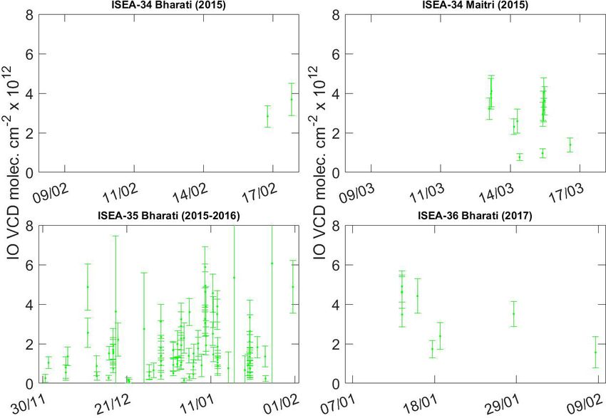
3.3 IO vertical column densities (VCDs) and mixing imum value during ISEA-35 and ISEA-36. In the case of
ratio profiles IO, there were far fewer valid retrieved profiles, as can be
seen in Fig. 7 (Fig. S6 shows all scans, including “bad” and
The O4 and IO DSCDs were used to retrieve the vertical “warning”). Only a total of 343 valid scans were retrieved
column densities and the vertical profiles for aerosols and for the vertical profiles of IO. One of the main reasons is
IO. A comparison of the MAX-DOAS-observed O4 DSCDs that for most of the scans the IO DSCDs at higher eleva-
with the MAPA-modeled DSCDs for all four campaigns are tion angles are below the detection limit and that not enough
shown in Fig. S3, and Fig. S4 shows a similar plot for the information is available for the model to retrieve a valid ver-
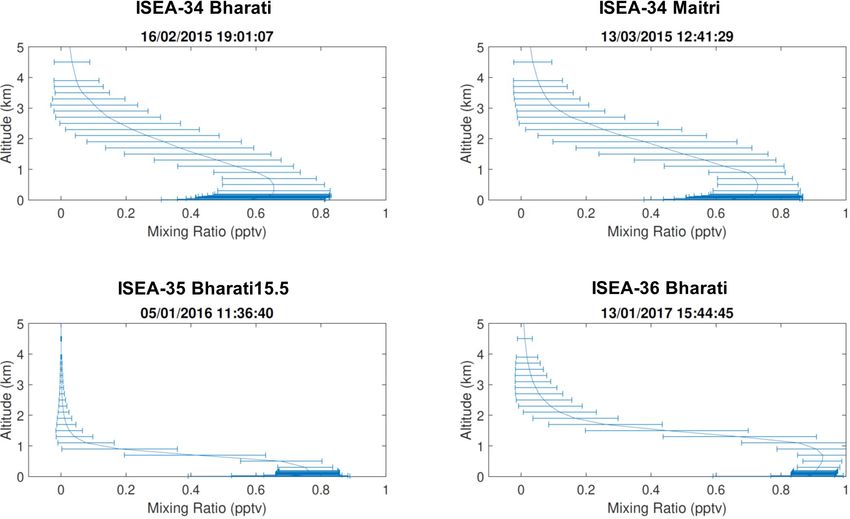
IO DSCDs. Figures 6 and 7 show the MAPA-calculated tical profile. In the case of IO VCDs, there were only two
aerosol optical depths (AODs) and IO VCDs, respectively, scans that showed a valid flag over the 10 d period during the
for all the campaigns. Several data points are flagged as er- ISEA-34 campaign at Bharati due to adverse weather condi-
rors or warnings, with a few scans giving a “valid” flag. In tions leading to mostly cloudy weather. Thus, the mean VCD
the case of aerosols, the warning or error flags are mainly value of 2.83×10¹² molec. cm−2 should be treated with some
for scans which were during cloudy weather (Fig. S5 shows caution. In Maitri during ISEA-34, the IO VCD ranged be-
the data which were flagged as “bad” and “warning” along tween 2.37×10¹² and 4.25×10¹² molec. cm−2 , with a mean
with the valid scans). As mentioned above, the cloud cover value of 3.40 ± 0.57 × 10¹² molec. cm−2 . During ISEA-35 at
was regularly measured throughout the campaigns as a part Bharati, which had the highest number of valid scans over the
of the meteorological observations. In addition to visual ob- four campaigns, the IO VCDs ranged between 0.01 × 10¹²
servations, we also computed the cloud index following past and 5.86 × 10¹² molec. cm−2 , with a mean value of 2.62 ±
works based on MAX-DOAS observations (Mahajan et al., 1.16 × 10¹² molec. cm−2 . During ISEA-36, the IO VCDs
2012; Wagner et al., 2014), which confirmed that the er- ranged between 2.78 × 10¹² and 4.90 × 10¹² molec. cm−2 ,
ror and warning flags were during cloud cover periods. For with a mean value of 3.92 ± 0.79 × 10¹² molec. cm−2 at
the valid scans, the AODs ranged between 0.002 and 0.016, Bharati (Table S1 in the Supplement).
with a mean value of 0.003 for ISEA-34 at Bharati; between In addition to the VCDs, vertical profiles of aerosols
0.001 and 0.067, with a mean value of 0.011 for ISEA-34 (Fig. S7) and IO were estimated using MAPA. Figure 8
at Maitri; between 0.001 and 1.866, with a mean value of shows the typical vertical profiles of IO mixing ratios over
0.037 for ISEA-35 at Bharati; and between 0.001 and 0.878, the four expeditions. The surface mixing ratios for the
with a mean value of 0.016 for ISEA-36 at Bharati (Fig. 6). valid scans across all the campaigns range between 0.2 and
The low values are expected considering the pristine con- 1.3 pptv (Table S1). The surface (< 30 m) concentrations ob-
ditions in Antarctica, although during a couple of scans el- served at both Maitri and Bharati are lower than observations
evated levels were observed as demonstrated by the max- in the Weddell Sea region, where summertime concentrations
https://doi.org/10.5194/acp-21-11829-2021 Atmos. Chem. Phys., 21, 11829–11842, 2021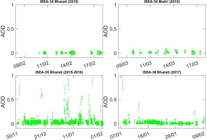
11836           A. S. Mahajan et al.: Observations of iodine monoxide over three summers at the Indian Antarctic bases

Figure 7. Observations of IO vertical column densities observed throughout all four campaigns are shown. These data were mostly during
periods of clear sky and where IO was observed above the detection limit for most of the set elevation angles, enabling a reliable profile
retrieval.

Figure 8. Typical examples of IO vertical profiles retrieved during all four campaigns are shown. The times are in UTC.

exceeding 6 pptv have been reported in the past (Atkinson et            pack using a long-path DOAS (LP-DOAS) instrument, was
al., 2012; Saiz-Lopez et al., 2007a), or at the Neumayer sta-           about 3 pptv, approximately a factor of 3 higher than the ob-
tion, where long-term zenith sky DOAS measurements of IO                servations at Bharati and Maitri. Considering that the MAX-
suggest mixing ratios as high as ∼ 10 pptv during the sum-              DOAS-retrieved profiles are not very sensitive to the lower-
mer (Frieß et al., 2001). It should be noted that although el-          most few meters, this difference is expected. This is because
evated concentrations were observed at Halley, the average              the source of IO is expected to be from the surface, and re-
summer concentration, measured only 4 m above the snow-                 mote sensing estimates have suggested that high IO concen-

Atmos. Chem. Phys., 21, 11829–11842, 2021                                                https://doi.org/10.5194/acp-21-11829-2021
A. S. Mahajan et al.: Observations of iodine monoxide over three summers at the Indian Antarctic bases 11837
trations on the order of 50 ppbv are present in the snow in-
terstitial air (Frieß et al., 2010), suggesting that snowpack is
indeed the source for iodine compounds. If this is the case, a
strong gradient would be observed considering the short life-
time of IO in the atmosphere, and hence the MAX-DOAS ob-
servations would be lower than the LP-DOAS observations.
However, this does not explain the large difference compared
to Neumayer, where the estimated value was 10 pptv. Indeed,
Maitri is close to Neumayer, and the reasons for the large
difference between the two sites remains a mystery. The ob-
servations reported in this study are also similar to measure-
ments at McMurdo Sound, near the Ross Sea, where MAX-
DOAS observations reported a maximum of 2.6 ± 0.1 pptv
with most of the observations below 1 pptv during 2006 and Figure 9. Averaged VCDs of IO retrieved by SCIAMACHY be-
2007 (Hay, 2010). It should be noted that the surface values tween 2004 and 2011 are shown. Observations suggest that lower
levels of IO are expected at Bharati and Maitri compared to Halley
were not highly weighted by the a priori values. McMurdo
Bay and Neumayer.
Sound is also located in the East Antarctic, which shows
lower levels of IO in the satellite estimates (Schönhardt et
al., 2008) and in models (Fernandez et al., 2019). is that the MAX-DOAS-observation-based profile retrievals
Vertical profiles of IO have been reported only once in typically get only a couple of points of information in the
the past for Antarctica. These measurements were made at boundary layer and are hence not expected to capture this
McMurdo Sound in East Antarctica (Hay, 2010). IO values strong decrease.
over 2 d in 2006 and 2007 show typical surface concentra-
tions of ∼ 1 pptv (with a maximum of 2.6 pptv), decreasing 3.4 Comparison with satellite-based estimates
to ∼ 0.2 pptv at about 200 m. A second maximum of 0.6 pptv
at ∼ 700 m was also observed, but the models do not repro- The satellite-based vertical column densities of IO across
duce this profile shape, and the observations were subject the Weddell Sea region and the region encompassing Bharati
to large uncertainties, with the vertical profile above 200 m and Maitri are shown in Fig. 9. The averaged satellite-based
dominated by the a priori values (Hay, 2010). During the four VCD observations suggest that lower levels of IO are ex-
campaigns studied here, elevated concentrations, similar to pected at both the Indian bases compared to places where
the surface, were usually observed until about 400 m. Above ground-based observations have been reported in the past,
this height, there is a decrease, with the retrievals reducing to such as Halley Bay and Neumayer. The mean and standard
below 0.1 pptv (Fig. 8). Although the boundary layer height deviation over the 8 years of observations for Bharati is
was not available for most of the days, radiosonde observa- 0.6 ± 0.5 × 10¹² molec. cm−2 , while for Maitri the amount
tions (not shown) show that the boundary layer height ranged is 0.5 ± 0.5 × 10¹² molec. cm−2 , each for the whole time se-
between 300 and 700 m. The means and their standard de- ries. For single months the values can be higher: the mean
viations for the lowest 400 m for the different campaigns IO VCD for Bharati is 0.8 or 0.4 × 10¹² molec. cm−2 in De-
are given in Table S1. The reducing standard deviations in cember or February, respectively, and 0.6×10¹² molec. cm−2
the profile retrieval with altitude show that all the profiles in March for Maitri. This is lower than the mean value of
which reproduce elevated IO close to the ground approach 2.62 ± 1.16 × 10¹² molec. cm−2 observed at Bharati during
zero for higher altitudes, suggesting that most of the IO is ISEA-35, which was the longest dataset available in this
within the lower part of the troposphere. However, this gra- study, suggesting that the ground-based instruments observe
dient is much more gradual than estimates predicted using larger VCDs compared to the satellite-based instruments.
the THAMO one-dimensional model at Halley Bay (Saiz- However, it should be noted that the SCIAMACHY data are
Lopez et al., 2008). In most models, the assumption is that an average over all the seasons, and individual daily data
the source is from the snowpack, and hence a strong decreas- points as high as 2.1×10¹² molec. cm−2 have been observed.
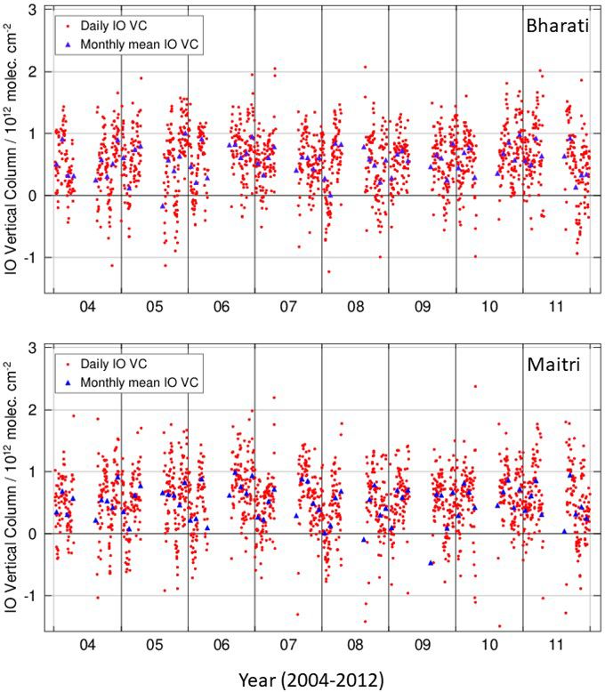
ing gradient with altitude has been predicted (Saiz-Lopez et Figure 10 shows the time series for Bharati and Maitri with
al., 2008). The gradient of this decrease depends on the pho- daily averages (red dots), as well as monthly averages (blue
tolysis of the higher oxides and on the recycling of iodine triangles), for the years 2004 to 2011. Satellite measurements
reservoir species in aerosols, both of which have uncertain- from within 500 km around the stations were included in the
ties. When the gradient was estimated in 2008 (Saiz-Lopez analysis. It should be mentioned that this spatial averaging
et al., 2008), the photolysis rates for the higher iodine ox- could cause the introduction of larger uncertainties due to
ides were not available, but this has recently been measured the heterogeneity in the IO distribution, but it is necessary to
in the laboratory (Lewis et al., 2020), and THAMO needs to improve the signal to noise.
be updated accordingly. Another important point to consider
https://doi.org/10.5194/acp-21-11829-2021 Atmos. Chem. Phys., 21, 11829–11842, 202111838 A. S. Mahajan et al.: Observations of iodine monoxide over three summers at the Indian Antarctic bases
is much lower. The use of a higher albedo would result in an
underestimation of the VCD by the satellite, which is the case
when compared to the ground-based instruments. At Maitri
this should not be the case considering that Maitri is 125 km
inland from the coast, and the ice shelf is less than 1 km from
the station along the light path. It should be noted that the
MAPA LUTs are calculated for a low surface albedo (5 %),
and hence, at least for some of the measurements, the sur-
face albedo is probably much higher, especially at Maitri. As
far as we understand, the effect of the surface albedo mainly
cancels out in the MAX-DOAS analysis, but it could be one
possible uncertainty in the retrieval results. Another reason
for the discrepancy between the ground-based and satellite-
retrieved VCDs could be the overpass time, which was ap-
proximately 09:00 LT. Although this should not be a large
factor during the summer months due to long sunlit hours
and given that the numbers provided above were averages
throughout the entire campaign for the ground-based obser-
vations, measurements at Halley Bay have shown a strong
diurnal profile peaking at noon (Saiz-Lopez et al., 2007a).
Hence, it is possible that the ground-based observations,
which are filtered for SZA > 75◦ , capture higher values than
the satellite.
Finally, a point to consider is that the satellite data avail-
Figure 10. Time series of IO VCD observations at Bharati station
retrieved by SCIAMACHY. The monthly mean values are shown in
able from SCIAMACHY is for the period of 2004–2011,
blue, and the daily data points are shown in red. whereas the MAX-DOAS observations were conducted over
three summers from 2015 to 2017. This temporal discrep-
ancy, although small considering the long satellite dataset,
could contribute to the difference in the retrieved VCDs. Re-
When the whole IO column is constrained to the lower cent observations of iodine in ice cores in the Alpine region
400 m, the satellite-retrieved VCDs translate to a range be- and over Greenland have shown an increasing trend for at-
tween 0.6 and 1.3 pptv. The daily satellite VCDs tend to mospheric iodine in the Northern Hemisphere (Cuevas et al.,
exceed these averaged values and result in mixing ratios as 2018; Legrand et al., 2018). In the Antarctic only seasonal
high as 2 pptv. This is similar to the range observed through- and geographical variations in halogens in the ice have been
out the four campaigns reported here. However, observations studied, and no long-term dataset is available (Vallelonga et
during the springtime were not made over these four cam- al., 2017). The main cause for this increase is suggested to be
paigns, when emissions of iodine species have been shown an increase in tropospheric ozone, which drives the emission
to peak at Halley Bay (Saiz-Lopez et al., 2007a). During the of iodine compounds from the ocean surface through het-
spring season, values as high as 20 pptv were observed at erogenous chemistry at the ocean interstitial surface (Carpen-
Halley Bay, a factor of 10 higher than during the summer at ter et al., 2013). Although questions regarding the strength
the Indian stations. However, the satellite observations do not of this inorganic source in affecting IO concentrations in the
show a large peak over the springtime over both Indian sta- Southern Ocean remain (Inamdar et al., 2020; Mahajan et
tions. Another outstanding question is whether the satellites al., 2019), it is possible that the discrepancy between the
are sensitive to the lower 100–200 m, considering the strong satellite- and ground-based data is because of a different time
gradient in IO. Figure S8 shows the block AMFs for satellite period. However, no increasing trend was observed in the
retrievals demonstrating a significant difference between the satellite data for the period between 2004 and 2011 (Fig. 10),
block AMFs over Antarctica at different albedo values. Over which suggests that a factor of 3 increase in the VCDs is most
the ice-covered regions in Antarctica, the satellite is sensitive likely due to a difference in the measurement technique and
to the lower troposphere as the albedo is usually 0.9 or above. sensitivities rather than a change in the emissions.
Observations have shown that open water has an albedo of
0.05–0.2 (Jin et al., 2004), whereas the albedo of sea ice 3.5 Air mass origin dependence
ranges between 0.6 and 0.7 for bare ice and 0.8–0.9 for snow-
covered ice (Perovich et al., 2002). In the case of Bharati, Year-long observations at Halley Bay in West Antarctica,
Quilty Bay is not ice-covered during the summer, and hence which were made using the LP-DOAS instrument, sug-
along the light path in Bharati, the sensitivity of the satellite gested a oceanic primary source (Saiz-Lopez et al., 2007a).
Atmos. Chem. Phys., 21, 11829–11842, 2021 https://doi.org/10.5194/acp-21-11829-2021A. S. Mahajan et al.: Observations of iodine monoxide over three summers at the Indian Antarctic bases 11839
The authors showed through the tracking of air mass back- we still do not understand iodine chemistry in the polar re-
trajectories that elevated levels of IO were present in air gions. This study suggests that a longer dataset over different
masses that passed over the coastal and oceanic regions com- seasons and regions of Antarctica is necessary to answer the
pared to the air masses that had only continental exposures. outstanding questions regarding the sources and seasonal im-
However, even in air masses that had passed only over the portance of IO in the Indian Ocean sector of Antarctica.
continent for the past 5 d, the IO levels were still above
the detection limit, which suggested that even if the pri-
mary source is oceanic, a secondary source from the snow Code and data availability. All the MATLAB codes and
pack contributed to the atmospheric IO. Indeed, subsequent data used for analysis of this study are available at
studies have tried to explain the snowpack source through https://doi.org/10.17632/wvh25bxzpb.2 (Mahajan, 2021).
recycling of primary emissions from the ocean (Fernandez
et al., 2019), and one study has even suggested a strong
snowpack source based on simulated observations (Frieß et Supplement. The supplement related to this article is available on-
line at: https://doi.org/10.5194/acp-21-11829-2021-supplement.
al., 2010). Although the levels of IO are much lower than
the peak concentrations seen at Halley Bay, we studied the
back-trajectories to see if the origin of air masses leads to
Author contributions. ASM conceptualized the research plan and
a difference in the observed IO levels at both Bharati and methodology, did the analysis, and wrote the manuscript. MSB did
Maitri. Considering the short lifetime of reactive iodine com- the field observations. SB, TW, NB, and ASL helped with the inter-
pounds in the atmosphere, we calculated the exposure of each pretation of the observations, and AS provided the satellite obser-
HYSPLIT-calculated back-trajectory according to the region vations and helped interpret them.
it passed over in the last 12 h. Depending on where the tra-
jectories spend the most amount of time, they were classified
into coastal, continental, and oceanic air masses. The coastal Competing interests. The authors declare that they have no conflict
region was defined as a 0.5◦ belt along the Antarctic coast- of interest.
line, with regions to the north and south of this belt consid-
ered to be oceanic and continental even though most of them
had a coastal origin when the 5 d trajectories are considered Disclaimer. Publisher’s note: Copernicus Publications remains
(Fig. S9). Using the profiles which were valid, no clear de- neutral with regard to jurisdictional claims in published maps and
pendence on the air mass origin was observed. Indeed, most institutional affiliations.
of the data points at both stations corresponded to air masses
which were either coastal or continental (Fig. S10) and are
representative of the typical wind patterns during the sum- Acknowledgements. We thank the logistical and scientific teams of
the ISEA-34, ISEA-35, and ISEA-36 campaigns for enabling ob-
mer season. Thus, using this dataset, it was not possible to
servations throughout the expeditions. The ISEA campaigns are or-
draw any conclusions regarding the possible sources of IO in ganized by the National Centre for Polar and Ocean Research (NC-
this region, and a longer study is needed in the future. POR), Ministry of Earth Sciences (MOES), Government of India.
IITM and NCPOR are funded by MOES, Government of India.
4 Conclusions
Review statement. This paper was edited by Jayanarayanan Kuttip-
This study presents observations of iodine oxide (IO) at the purath and reviewed by one anonymous referee.
Indian Antarctic bases of Maitri and Bharati made over three
summers from 2015 through 2017. IO was observed inter-
mittently during all the campaigns with mixing ratios below
2 pptv. Using a profile retrieval algorithm, vertical gradients
of IO were estimated, and these showed a decreasing pro-
file with a peak in the boundary layer. The vertical profiles
confirmed the past hypothesis of a source from the ground
considering a sharp gradient. The vertical columns observed
using the ground-based instrument are approximately a fac-
tor of 3–5 higher than the climatological mean observed by
the satellite, which could be due to a difference in the mea-
surement techniques and sensitivities. Air mass origin anal-
ysis using back-trajectories did not lead to a conclusive an-
swer about the source regions. Indeed, it raises new questions
about comparisons with past observations, which show that
https://doi.org/10.5194/acp-21-11829-2021 Atmos. Chem. Phys., 21, 11829–11842, 202111840 A. S. Mahajan et al.: Observations of iodine monoxide over three summers at the Indian Antarctic bases
References Cuevas, C. A., Maffezzoli, N., Corella, J. P., Spolaor, A., Vallelonga,
P., Kjær, H. A., Simonsen, M., Winstrup, M., Vinther, B., Horvat,
C., Fernandez, R. P., Kinnison, D., Lamarque, J.-F., Barbante, C.,
Allan, J. D., Williams, P. I., Najera, J., Whitehead, J. D., Flynn, and Saiz-Lopez, A.: Rapid increase in atmospheric iodine levels
M. J., Taylor, J. W., Liu, D., Darbyshire, E., Carpenter, L. J., in the North Atlantic since the mid-20th century, Nat. Commun.,
Chance, R., Andrews, S. J., Hackenberg, S. C., and McFiggans, 9, 1452, https://doi.org/10.1038/s41467-018-03756-1, 2018.
G.: Iodine observed in new particle formation events in the Arctic Deutschmann, T., Beirle, S., Frieß, U., Grzegorski, M., Kern, C.,
atmosphere during ACCACIA, Atmos. Chem. Phys., 15, 5599– Kritten, L., Platt, U., Prados-Román, C., Pukite, J., Wagner, T.,
5609, https://doi.org/10.5194/acp-15-5599-2015, 2015. Werner, B., and Pfeilsticker, K.: The Monte Carlo atmospheric
Atkinson, H. M., Huang, R.-J., Chance, R., Roscoe, H. K., Hughes, radiative transfer model McArtim: Introduction and validation of
C., Davison, B., Schönhardt, A., Mahajan, A. S., Saiz-Lopez, Jacobians and 3D features, J. Quant. Spectrosc. Ra., 112, 1119–
A., Hoffmann, T., and Liss, P. S.: Iodine emissions from the sea 1137, https://doi.org/10.1016/j.jqsrt.2010.12.009, 2011.
ice of the Weddell Sea, Atmos. Chem. Phys., 12, 11229–11244, Draxler, R. and Rolph, G.: HYSPLIT (HYbrid Single Particle
https://doi.org/10.5194/acp-12-11229-2012, 2012. Lagrangian Integrated Trajectory). Model access via NOAA
Barrie, L. A., Bottenheim, J. W., Schnell, R. C., Crutzen, P. J., ARL Ready, online, available at: https://www.ready.noaa.gov/
and Rasmussen, R. A.: Ozone destruction and photochemical HYSPLIT.php (last access: 20 September 2020), 2003.
reactions at polar sunrise in the lower Arctic atmosphere, Na- Fayt, C. and Van Roozendael, M.: QDOAS 1.00. Software
ture, 334, 138–141, http://www.nature.com/nature/journal/v334/ User Manual, online, available at: http://uv-vis.aeronomie.be/
n6178/abs/334138a0.html (last access: 3 May 2012), 1988. software/QDOAS/ (last access: 20 September 2020), 2013.
Beirle, S., Dörner, S., Donner, S., Remmers, J., Wang, Y., and Fernandez, R. P., Carmona-Balea, A., Cuevas, C. A., Barrera, J.
Wagner, T.: The Mainz profile algorithm (MAPA), Atmos. A., Kinnison, D. E., Lamarque, J., Blaszczak-Boxe, C., Kim, K.,
Meas. Tech., 12, 1785–1806, https://doi.org/10.5194/amt-12- Choi, W., Hay, T., Blechschmidt, A., Schönhardt, A., Burrows,
1785-2019, 2019. J. P., and Saiz-Lopez, A.: Modeling the Sources and Chemistry
Bogumil, K., Orphal, J., Homann, T., Voigt, S., Spietz, P., Fleis- of Polar Tropospheric Halogens (Cl, Br, and I) Using the CAM-
chmann, O. C., Vogel, A., Hartmann, M., Kromminga, H., Chem Global Chemistry-Climate Model, J. Adv. Model. Earth
Bovensmann, H., Frerick, J., and Burrows, J. P.: Measurements Sy., 11, 2259–2289, https://doi.org/10.1029/2019MS001655,
of molecular absorption spectra with the SCIAMACHY pre- 2019.
flight model: instrument characterization and reference data for Fogelqvist, E. and Tanhua, T.: Iodinated C1–C4 hydrocarbons re-
atmospheric remote-sensing in the 230–2380 nm region, J. Pho- leased from ice algae in Antarctica BT – Naturally-Produced
toch. Photobio. A, 157, 167–184, https://doi.org/10.1016/S1010- Organohalogens, edited by: Grimvall, A. and de Leer, E. W. B.,
6030(03)00062-5, 2003. 295–305, Springer Netherlands, Dordrecht, 1995.
Bottenheim, J. W., Gallant, A. G., and Brice, K. A.: Measurements Frieß, U., Wagner, T., Pundt, I., Pfeilsticker, K., Platt, U., and Friefi,
of NOy Species and O3 at 82-Degrees-N Latitude, Geophys. Res. U.: Spectroscopic Measurements of Tropospheric Iodine Oxide
Lett., 13, 113–116, 1986. at Neumayer Station, Antarctica, Geophys. Res. Lett., 28, 1941–
Burrows, J. P., Hölzle, E., Goede, A. P. H., Visser, H., and Fricke, 1944, 2001.
W.: SCIAMACHY – Scanning Imaging Absorption Spectrome- Frieß, U., Deutschmann, T., Gilfedder, B. S., Weller, R., and
ter for Atmospheric Chartography, Acta Astronaut., 35, 445–451, Platt, U.: Iodine monoxide in the Antarctic snowpack, Atmos.
1995. Chem. Phys., 10, 2439–2456, https://doi.org/10.5194/acp-10-
Buys, Z., Brough, N., Huey, L. G., Tanner, D. J., von Glasow, 2439-2010, 2010.
R., and Jones, A. E.: High temporal resolution Br2 , BrCl and Garrison, D. L. and Buck, K. R.: The biota of Antarctic pack ice in
BrO observations in coastal Antarctica, Atmos. Chem. Phys., 13, the Weddell sea and Antarctic Peninsula regions, Polar Biol., 10,
1329–1343, https://doi.org/10.5194/acp-13-1329-2013, 2013. 211–219, https://doi.org/10.1007/BF00238497, 1989.
Carpenter, L. J., Wevill, D. J., Palmer, C. J., and Michels, J.: Depth Gómez Martín, J. C., Spietz, P., and Burrows, J. P.: Spectroscopic
profiles of volatile iodine and bromine-containing halocarbons in studies of the I-2/O-3 photochemistry – Part 1: Determination
coastal Antarctic waters, Mar. Chem., 103, 227–236, 2007. of the absolute absorption cross sections of iodine oxides of
Carpenter, L. J., MacDonald, S. M., Shaw, M. D., Kumar, atmospheric relevance, J. Photoch. Photobio. A, 176, 15–38,
R., Saunders, R. W., Parthipan, R., Wilson, J., and Plane, https://doi.org/10.1016/j.jphotochem.2005.09.024, 2005.
J. M. C.: Atmospheric iodine levels influenced by sea sur- Grilli, R., Legrand, M., Kukui, A., Méjean, G., Preunkert, S., and
face emissions of inorganic iodine, Nat. Geosci., 6, 108–111, Romanini, D.: First investigations of IO, BrO, and NO2 summer
https://doi.org/10.1038/ngeo1687, 2013. atmospheric levels at a coastal East Antarctic site using mode-
Chance, K. V and Spurr, R. J.: Ring effect studies: Rayleigh scatter- locked cavity enhanced absorption spectroscopy., Geophys. Res.
ing, including molecular parameters for rotational Raman scat- Lett., 40, 791–796, https://doi.org/10.1002/GRL.50154, 2013.
tering, and the Fraunhofer spectrum., Appl. Opt., 36, 5224–5230, Hay, T.: MAX – DOAS measurements of bromine explosion events
1997. in McMurdo Sound, Antarctica, University of Canterbury, Can-
Chaubey, J. P., Krishna Moorthy, K., Suresh Babu, S., and Nair, V. terbury, 2010.
S.: The optical and physical properties of atmospheric aerosols Hollwedel, J., Wenig, M., Beirle, S., Kraus, S., Kühl, S., Wilms-
over the Indian Antarctic stations during southern hemispheric Grabe, W., Platt, U., and Wagner, T.: Year-to-Year Variability of
summer of the International Polar Year 2007–2008, Ann. Geo- Polar Tropospheric BrO as seen by GOME, Adv. Space Res., 34,
phys., 29, 109–121, https://doi.org/10.5194/angeo-29-109-2011, 804–808, https://doi.org/10.1016/j.asr.2003.08.060, 2004.
2011.
Atmos. Chem. Phys., 21, 11829–11842, 2021 https://doi.org/10.5194/acp-21-11829-2021A. S. Mahajan et al.: Observations of iodine monoxide over three summers at the Indian Antarctic bases 11841 Hönninger, G., von Friedeburg, C., and Platt, U.: Multi axis dif- in the wavelength range 225–375 nm, J. Geophys. Res., 105, ferential optical absorption spectroscopy (MAX-DOAS), At- 7089–7101, https://doi.org/10.1029/1999JD901074, 2000. mos. Chem. Phys., 4, 231–254, https://doi.org/10.5194/acp-4- O’Dowd, C. D., Facchini, M. C., Cavalli, F., Ceburnis, 231-2004, 2004. D., Mircea, M., Decesari, S., Fuzzi, S., Yoon, Y. J., Inamdar, S., Tinel, L., Chance, R., Carpenter, L. J., Sabu, P., Putaud, J. P., and Dowd, C. D. O.: Biogenically driven or- Chacko, R., Tripathy, S. C., Kerkar, A. U., Sinha, A. K., Bhaskar, ganic contribution to marine aerosol, Nature, 431, 676–680, P. V., Sarkar, A., Roy, R., Sherwen, T., Cuevas, C., Saiz-Lopez, https://doi.org/10.1038/nature02959, 2004. A., Ram, K., and Mahajan, A. S.: Estimation of reactive in- Oltmans, S. J. and Komhyr, W. D.: Surface Ozone Distributions and organic iodine fluxes in the Indian and Southern Ocean ma- Variations from 1973–1984 Measurements at the Noaa Geophys- rine boundary layer, Atmos. Chem. Phys., 20, 12093–12114, ical Monitoring for Climatic-Change Base-Line Observatories, J. https://doi.org/10.5194/acp-20-12093-2020, 2020. Geophys. Res.-Atmos., 91, 5229–5236, 1986. Jin, Z., Charlock, T. P., Smith, W. L., and Rutledge, K.: A parame- Perovich, D. K., Grenfell, T. C., Light, B., and Hobbs, P. terization of ocean surface albedo, Geophys. Res. Lett., 31, 1–4, V.: Seasonal evolution of the albedo of multiyear Actic sea https://doi.org/10.1029/2004GL021180, 2004. ice, J. Geophys. Res.–Oceans, 107, SHE 20-1–SHE 20-13, Koenig, T. K., Baidar, S., Campuzano-Jost, P., Cuevas, C. A., https://doi.org/10.1029/2000jc000438, 2002. Dix, B., Fernandez, R. P., Guo, H., Hall, S. R., Kinnison, Platt, U. and Stutz, J.: Differential optical absorption spectroscopy: D., Nault, B. A., Ullmann, K., Jimenez, J. L., Saiz-Lopez, Principles and applications, First Ed., Springer-Verlag, Berlin, A., and Volkamer, R.: Quantitative detection of iodine in Heidelberg, https://doi.org/10.1007/978-3-540-75776-4, 2008. the stratosphere, P. Natl. Acad. Sci. USA, 15, 201916828, Raso, A. R. W., Custard, K. D., May, N. W., Tanner, D., Newburn, https://doi.org/10.1073/pnas.1916828117, 2020. M. K., Walker, L., Moore, R. J., Huey, L. G., Alexander, L., Shep- Kreher, K., Johnston, P. V., Wood, S. W., Nardi, B., and Platt, U.: son, P. B., and Pratt, K. A.: Active molecular iodine photochem- Ground-based measurements of tropospheric and stratospheric istry in the Arctic, P. Natl. Acad. Sci. USA, 114, 10053–10058, BrO at Arrival Heights, Antarctica, Geophys. Res. Lett., 24, https://doi.org/10.1073/pnas.1702803114, 2017. 3021–3024, https://doi.org/10.1029/97GL02997, 1997. Reifenhäuser, W. and Heumann, K. G.: Determinations of methyl- Legrand, M., McConnell, J. R., Preunkert, S., Arienzo, M., Chell- iodine in the antarctic atmosphere at the south polar sea, Atmos. man, N., Gleason, K., Sherwen, T., Evans, M. J., and Carpen- Environ. A-Gen., 26, 2905–2912, 1992. ter, L. J.: Alpine ice evidence of a three-fold increase in atmo- Richter, A., Wittrock, F., Ladstätter-Weißenmayer, A., and Burrows, spheric iodine deposition since 1950 in Europe due to increasing J. P.: GOME measurements of stratospheric and tropospheric oceanic emissions, P. Natl. Acad. Sci. USA, 115, 12136–12141, BrO, Adv. Space Res., 29, 1667–1672, 2002. https://doi.org/10.1073/pnas.1809867115, 2018. Rothman, L. S., Gordon, I. E., Babikov, Y., Barbe, A., Chris Lewis, T. R., Gómez Martín, J. C., Blitz, M. A., Cuevas, C. Benner, D., Bernath, P. F., Birk, M., Bizzocchi, L., Boudon, A., Plane, J. M. C., and Saiz-Lopez, A.: Determination of V., Brown, L. R., Campargue, A., Chance, K., Cohen, E. a., the absorption cross sections of higher-order iodine oxides Coudert, L. H., Devi, V. M., Drouin, B. J., Fayt, A., Flaud, at 355 and 532 nm, Atmos. Chem. Phys., 20, 10865–10887, J.-M., Gamache, R. R., Harrison, J. J., Hartmann, J.-M., Hill, https://doi.org/10.5194/acp-20-10865-2020, 2020. C., Hodges, J. T., Jacquemart, D., Jolly, A., Lamouroux, J., Mahajan, A.: Data as a part of Observations of iodine Le Roy, R. J., Li, G., Long, D. a., Lyulin, O. M., Mackie, monoxide over three summers at the Indian Antarctic C. J., Massie, S. T., Mikhailenko, S., Müller, H. S. P., Nau- bases, Bharati and Maitri, [data set], Mendeley Data, V2, menko, O. V., Nikitin, A. V., Orphal, J., Perevalov, V., Per- https://doi.org/10.17632/wvh25bxzpb.2, 2021. rin, A., Polovtseva, E. R., Richard, C., Smith, M. a. H., Mahajan, A. S., Shaw, M., Oetjen, H., Hornsby, K. E., Carpen- Starikova, E., Sung, K., Tashkun, S., Tennyson, J., Toon, G. C., ter, L. J., Kaleschke, L., Tian-Kunze, X., Lee, J. D., Moller, Tyuterev, V. G., and Wagner, G.: The HITRAN 2012 molecu- S. J., Edwards, P. M., Commane, R., Ingham, T., Heard, D. lar spectroscopic database, J. Quant. Spectrosc. Ra., 130, 4–50, E., and Plane, J. M. C.: Evidence of reactive iodine chemistry https://doi.org/10.1016/j.jqsrt.2013.07.002, 2013. in the Arctic boundary layer, J. Geophys. Res., 115, D20303, Saiz-Lopez, A. and Blaszczak-boxe, C. S.: The po- https://doi.org/10.1029/2009JD013665, 2010. lar iodine paradox, Atmos. Environ., 145, 72–73, Mahajan, A. S., Gómez Martín, J. C., Hay, T. D., Royer, S.-J., https://doi.org/10.1016/j.atmosenv.2016.09.019, 2016. Yvon-Lewis, S., Liu, Y., Hu, L., Prados-Roman, C., Ordóñez, Saiz-Lopez, A. and von Glasow, R.: Reactive halogen chem- C., Plane, J. M. C., and Saiz-Lopez, A.: Latitudinal distribu- istry in the troposphere., Chem. Soc. Rev., 41, 6448–6472, tion of reactive iodine in the Eastern Pacific and its link to https://doi.org/10.1039/C2CS35208G, 2012. open ocean sources, Atmos. Chem. Phys., 12, 11609–11617, Saiz-Lopez, A., Mahajan, A. S., Salmon, R. A., Bauguitte, S. J.- https://doi.org/10.5194/acp-12-11609-2012, 2012. B., Jones, A. E., Roscoe, H. K., and Plane, J. M. C.: Boundary Mahajan, A. S., Tinel, L., Hulswar, S., Cuevas, C. A., Wang, S., Layer Halogens in Coastal Antarctica, Science, 317, 348–351, Ghude, S., Naik, R. K., Mishra, R. K., Sabu, P., Sarkar, A., https://doi.org/10.1126/science.1141408, 2007a. Anilkumar, N., and Saiz Lopez, A.: Observations of iodine ox- Saiz-Lopez, A., Chance, K. V., Liu, X., Kurosu, T. P., and Sander, ide in the Indian Ocean marine boundary layer: A transect from S. P.: First observations of iodine oxide from space, Geophys. the tropics to the high latitudes, Atmos. Environ. X, 1, 100016, Res. Lett., 34, L12812, https://doi.org/10.1029/2007GL030111, https://doi.org/10.1016/j.aeaoa.2019.100016, 2019. 2007b. Meller, R. and Moortgat, G. K.: Temperature dependence of the ab- Saiz-Lopez, A., Plane, J. M. C., Mahajan, A. S., Anderson, P. S., sorption cross sections of formaldehyde between 223 and 323 K Bauguitte, S. J.-B., Jones, A. E., Roscoe, H. K., Salmon, R. https://doi.org/10.5194/acp-21-11829-2021 Atmos. Chem. Phys., 21, 11829–11842, 2021
You can also read