Alkenone isotopes show evidence of active carbon concentrating mechanisms in coccolithophores as aqueous carbon dioxide concentrations fall below ...
←
→
Page content transcription
If your browser does not render page correctly, please read the page content below
Biogeosciences, 18, 1149–1160, 2021
https://doi.org/10.5194/bg-18-1149-2021
© Author(s) 2021. This work is distributed under
the Creative Commons Attribution 4.0 License.

Alkenone isotopes show evidence of active carbon concentrating
mechanisms in coccolithophores as aqueous carbon dioxide
concentrations fall below 7 µmol L−1
Marcus P. S. Badger
School of Environment, Earth & Ecosystem Sciences, The Open University, Milton Keynes, MK7 6AA, UK

Correspondence: Marcus P. S. Badger (marcus.badger@open.ac.uk)

Received: 25 September 2020 – Discussion started: 2 October 2020
Revised: 6 January 2021 – Accepted: 8 January 2021 – Published: 15 February 2021

Abstract. Coccolithophores and other haptophyte algae ac-       ganisms which live exclusively in the photic zone, alkenones
quire the carbon required for metabolic processes from the      allow probing of algal biogeochemistry, and as alkenones are
water in which they live. Whether carbon is actively moved      often preserved in the sedimentary record, alkenones can also
across the cell membrane via a carbon concentrating mecha-      provide information about past environmental conditions.
nism, or passively through diffusion, is important for hapto-      Two main proxy systems based on alkenone geochemistry
phyte biochemistry. The possible utilization of carbon con-     exist: one allows reconstruction of sea surface temperature
centrating mechanisms also has the potential to over-print      (SST) and relies on the changing degree of unsaturation of
                                                                                       0
one proxy method by which ancient atmospheric CO2 con-          the C37 alkenone (UK  37 ) (Brassell et al., 1986), whilst a sec-
centration is reconstructed using alkenone isotopes. Here       ond for atmospheric CO2 concentration is based on recon-
I show that carbon concentrating mechanisms are likely          structing the isotopic fractionation which takes place dur-
used when aqueous carbon dioxide concentrations are be-         ing photosynthesis (εp ) (Laws et al., 1995; Bidigare et al.,
low 7 µmol L−1 . I compile published alkenone-based CO2         1997). It is the second system using the stable carbon iso-
reconstructions from multiple sites over the Pleistocene and    topic composition of the preserved alkenones for reconstruct-
recalculate them using a common methodology, which al-          ing atmospheric CO2 concentration (referred to throughout
lows comparison to be made with ice core CO2 records.           as CO2(εp −alk) ) which is the focus of this study.
Interrogating these records reveals that the relationship be-      In the modern ocean, alkenones are produced primar-
tween proxy CO2 and ice core CO2 breaks down when lo-           ily by two dominant coccolithophore species: Emiliania
cal aqueous CO2 concentration falls below 7 µmol L−1 . The      huxleyi and Gephyrocapsa oceanica. E. huxleyi first ap-
recognition of this threshold explains why many alkenone-       peared 290 kyr ago and began to dominate over G. ocean-
based CO2 records fail to accurately replicate ice core CO2     ica around 82 kyr ago (Gradstein et al., 2012; Raffi et al.,
records, and it suggests the alkenone proxy is likely robust    2006). However alkenones are commonly found in sediments
for much of the Cenozoic when this threshold was unlikely       throughout the Cenozoic, with the oldest reported detections
to be reached in much of the global ocean.                      from mid-Albian-aged black shales (Farrimond et al., 1986).
                                                                Prior to the evolution of G. oceanica, alkenones were most
                                                                likely produced by other closely related species from the
                                                                Noelaerhabdaceae family (Marlowe et al., 1990; Volkman,
1   Introduction                                                2000). Micropalaeontological and molecular data split the
                                                                coccolith-bearing haptophytes into two distinct phylogenetic
Alkenones are long-chain (C37−39 ) ethyl and methyl ketones     clades: the Isochrysidales and Coccolithales. The Isochrysi-
(Fig. 1; Brassell et al., 1986; Rechka and Maxwell, 1987)       dales contain the modern alkenone-producing taxa, includ-
produced by a restricted group of photosynthetic haptophyte     ing E. huxleyi and G. oceanica, and fossil reticulofenestrids.
algae (Conte et al., 1994). Produced by a narrow group of or-   Meanwhile the non-alkenone-producers are separated into

Published by Copernicus Publications on behalf of the European Geosciences Union.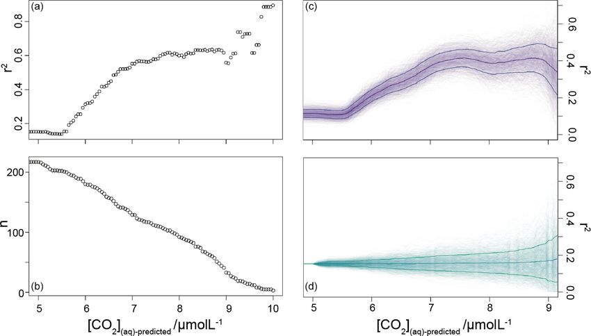
1150                                                                 M. P. S. Badger: CCMs in coccolithophores at low CO2

the order Coccolithales, which includes Coccolithus pelag-
icus and Calcidiscus leptoporus along with most other coc-
colithophores.
   Proxies for atmospheric CO2 concentration – includ-
ing CO2(εp −alk) , those based on the δ 11 B of planktic
foraminifera, geochemical modelling, and stomatal density
– broadly agree that over the Cenozoic atmospheric pCO2
declined from high levels (> 1000 µatm) in the “greenhouse”
worlds of the Palaeocene and Eocene to close to modern-
day values (around 400 µatm) in the Pliocene (Pagani et al.,
2005, 2011; Pearson et al., 2009; Anagnostou et al., 2016;
Foster et al., 2017; Sosdian et al., 2018; Super et al., 2018;      Figure 1. Alkenones are C37 unsaturated methyl ketones (Brassell
Zhang et al., 2013; Beerling and Royer, 2011). However, re-         et al., 1986; Rechka and Maxwell, 1987).
cently discrepancies have emerged between CO2(εp −alk) and
other CO2 proxies at the < 400 µatm atmospheric CO2 con-
centrations of the Pleistocene (i.e. Badger et al., 2019, 2013a,
and compare Badger et al., 2013b, and Pagani et al., 2009,          through water and the slow kinetics of the bicarbonate-to-
with Martínez-Botí et al., 2015). Whilst the long-standing          [CO2 ](aq) transformation, surface water [CO2 ](aq) can still be
differences between alkenone (Pagani et al., 1999), δ 11 B          depleted by photosynthetic activity. This can become partic-
(Foster et al., 2012), and stomatal proxies (Kürschner et al.,      ularly problematic in species which form blooms and at the
2008) in the Miocene CO2 reconstructions have been par-             cell boundary of species with limited motility. It should be
tially resolved with new SST records (Super et al., 2018),          no surprise therefore that many marine photosynthetic organ-
differences remain in the Pliocene (Pagani et al., 2009; Bad-       isms have evolved with mechanisms to concentrate carbon
ger et al., 2013b; Martínez-Botí et al., 2015) and Pleistocene      within the cell.
(Badger et al., 2019).                                                 The enzyme carbonic anhydrase (CA) can catalyse the de-
                                                                    hydration of HCO−   3 to [CO2 ](aq) to speed up availability of
Carbon concentrating mechanisms                                     carbon if the [CO2 ](aq) reservoir is depleted and has been
                                                                    observed in several haptophytes, including coccolithophores
One plausible reason for the discrepancies between                  (Rost et al., 2003; Riebesell et al., 2007). The exact contribu-
CO2(εp −alk) and other proxies for atmospheric CO2 is               tion of CA remains unclear, but two possible mechanisms for
the operation of active carbon concentrating mechanisms             CCMs have been postulated (Reinfelder, 2011): (1) CA catal-
(CCMs) in haptophytes. These are potentially important as           yses dehydration of HCO−     3 at the cell surface, which then
CO2(εp −alk) assumes purely passive uptake of carbon into           allows increased CO2 to diffuse into the cell passively, and
the haptophyte cell purely via diffusion (Laws et al., 1995;        (2) HCO−  3 is transported into the cell and then converted by
Bidigare et al., 1997). The potential for CCMs to affect            CA. Both of these options will likely impact the CO2(εp −alk)
CO2(εp −alk) has long been known (Laws et al., 1997, 2002;          proxy, firstly by changing the effective [CO2 ](aq) within the
Cassar et al., 2006), and recent work has refocussed ef-            cell (and so impacting εp ) and secondly by imparting another
forts on understanding CCMs in CO2(εp −alk) (Bolton et al.,         carbon isotopic fractionation during CA catalysation which
2012; Bolton and Stoll, 2013; Stoll et al., 2019; Zhang et al.,     is not considered by the CO2(εp −alk) proxy system. However
2019, 2020). Coccolithophores are thought to have low-              CA activity in coccolithophores does not appear to be regu-
efficiency CCMs – especially compared to diatoms, dinoflag-         lated by CO2 as it is in diatoms and Phaeocystis (Rost et al.,
ellates, and Phaeocystis – with evidence that CCMs play             2003), which may indicate a less-well-developed CCM in
a minor role in coccolithophore biochemistry in the CO2 -           coccolithophores.
replete worlds of the early Cenozoic (Bolton et al., 2012; Re-         Calcifying coccolithophores (which include alkenone pro-
infelder, 2011). Direct evidence from experimentation with          ducers E. huxleyi and G. oceanica) may be able to utilize
the marine diatom Phaeodactylum tricornutum suggests that           HCO−  3 directly as a carbon source (Trimborn et al., 2007),
both passive diffusive uptake and active CCMs operate at            with precipitation of CaCO3 providing an acid for the de-
the same time, with active uptake used to moderate inter-           hydration of HCO−   3 , but this still requires sufficient HCO3
                                                                                                                                   −
nal cell CO2 concentrations to minimize energy use during           entering the cell, and it is unclear whether calcification aids
transport to carboxylation sites (Laws et al., 1997). CO2 , un-     DIC acquisition (Riebesell et al., 2000; Zondervan et al.,
like some other nutrients, is abundant within the water col-        2002). The light-dependent leak of carbon (as CO2 and DIC)
umn, especially when considering the dissolved inorganic            back from haptophyte cells (including the coccolithophore
carbon (DIC) reservoir which includes bicarbonate (HCO−      3 ),   E. huxleyi) to seawater (Tchernov et al., 2003) suggests that
carbonate (CO2− 3 ), and dissolved CO 2 ([CO   ]
                                              2 (aq) ). However,    CCMs are energy intensive and can concentrate DIC within
due to the relatively slow diffusion of dissolved [CO2 ](aq)        the cell. Even with active CCMs, it appears that in the ocean

Biogeosciences, 18, 1149–1160, 2021                                                    https://doi.org/10.5194/bg-18-1149-2021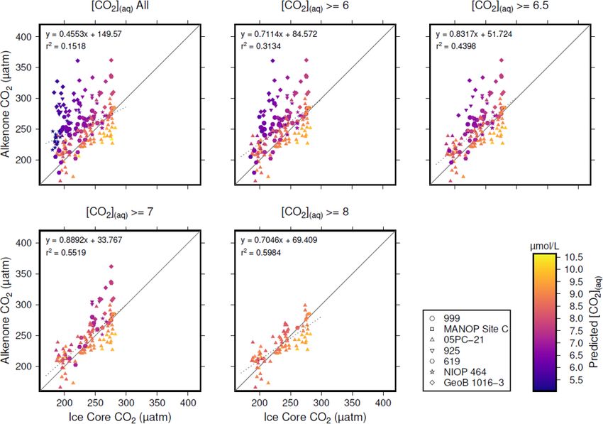
M. P. S. Badger: CCMs in coccolithophores at low CO2                                                                                   1151

coccolithophores are CO2 limited under some circumstances
(Riebesell et al., 2007).

2   Materials and methods

Calculating CO2 from alkenone δ 13 C values: the
CO2(εp −alk) proxy

In this study I use the now large number of published
CO2(εp −alk) records which overlap with ice core records of
atmospheric CO2 concentration (Tables 1 and 2) to explore
the relationship between CO2(εp −alk) and CCMs in the Pleis-
tocene, where our understanding of atmospheric CO2 con-
centration is best.                                                  Figure 2. Study sites relative to mean annual surface ocean CO2
    Multiple records of CO2(εp −alk) have been published for         disequilibrium for 2005. Sites are globally distributed in longitude
the Pleistocene (Fig. 2, Table 1), allowing direct comparison        but restricted in latitude, as generally sites are chosen to be close to
                                                                     surface water equilibrium with the atmosphere. Sites used for this
with ice-core-based CO2 records (Table 2). These records are
                                                                     study are indicated, over the mean annual surface ocean disequilib-
globally distributed in longitude but are concentrated at low-       rium for 2005 calculated from Takahashi et al. (2014). The MANOP
latitude sites, largely as there is a general preference for sites   Site C (Jasper et al., 1994) was chosen to study the disequilibrium
which have (in the modern ocean) surface waters close to             at that site, so it is shown here but not used in the following anal-
equilibrium with the atmosphere (Fig. 2, Table 1). In longer-        yses. Site symbols are used throughout the figures: ODP 999 – cir-
term palaeoclimate studies there has also been a preference          cle; 05PC-21 – triangle; ODP 925 – inverted triangle; DSDP 619
for low-latitude gyre sites in the belief that these sites are       – hexagon; MANOP Site C – square; NIOP 464 – star; and GeoB
more likely to be oceanographically stable over long time in-        1016-3 – diamond.
tervals (Pagani et al., 1999). Most of the records included
here (Table 1, Fig. 2) were generated with the aim to re-
construct atmospheric CO2 concentration; however one, the            solved CO2 (δ 13 CCO2(aq) ) and haptophyte biomass (δ 13 Corg ).
MANOP Site C of Jasper et al. (1994), was used to explicitly         The isotopic fractionation between δ 13 Calkenone and δ 13 Corg
reconstruct changing disequilibrium due to oceanographic             is first corrected assuming a constant fractionation (εalkenone )
frontal changes over time and so is excluded from the fol-           of 4.2 ‰ (Garcia et al., 2013; Popp et al., 1998; Bidigare
lowing analysis.                                                     et al., 1997):
    Whilst these sites do only span a relatively small latitu-
                                                                                   δ 13 Calkenone + 1000
dinal extent, the diversity of settings does allow for investi-      εalkenone =                         − 1.                            (1)
gation of any secondary controls on alkenone δ 13 C values                            δ 13 Corg + 1000
(δ 13 Calkenone ) – in particular, differences in oceanographic
                                                                        The isotopic composition of DIC is estimated using
setting and SST to test the hypothesis that low [CO2 ](aq)
                                                                     (ideally) the δ 13 C value of planktic foraminifera and the
breaks the relationship between δ 13 Calkenone and atmospheric
                                                                     temperature-dependent fractionation between calcite and
CO2 concentration, as might be expected if haptophytes
                                                                     [CO2 ](g) experimentally determined by Romanek et al.
are able to actively take up carbon from seawater to meet
                                                                     (1992), where T is sea surface temperature in degrees Cel-
metabolic demand (i.e. activate CCMs).
                                                                     sius (SST):
    To facilitate fair comparison between sites and consistent
comparison with the ice core records, all CO2(εp −alk) records       εcalcite−CO2(g) = 11.98 − 0.12T .                                   (2)
were recalculated using a consistent approach. The approach
is based on Bidigare et al. (1997), which updated the initial            The value of the carbon isotopic composition of CO2(g)
approach of Jasper and Hayes (1990) to CO2(εp −alk) . This           (δ 13 CCO2(g) ) can then be calculated:
approach removes some additional corrections used in the
original publication of the records (such as growth rate ad-                            δ 13 Ccarbonate + 1000
justment for NIOP 464; Palmer et al., 2010) but does allow           δ 13 CCO2(g) =                             − 1000.                  (3)
                                                                                      εcalcite−CO2(g) /1000 + 1
for direct comparison to be made. For all sites the “b” term
was estimated using modern-day surface [PO3−       4 ] (Bidigare       From this δ 13 CCO2(aq) can be calculated using the relation-
et al., 1997; Pagani et al., 2009)
                                                                     ship experimentally determined by Mook et al. (1974),
    An overview of how CO2(εp −alk) data are typically gener-
ated is given in Badger et al. (2013b). Briefly, to calculate                               −373
εp requires the stable carbon isotopic composition of the dis-       εCO2(aq) −CO2(g) =              + 0.19,                             (4)
                                                                                          T + 273.15

https://doi.org/10.5194/bg-18-1149-2021                                                        Biogeosciences, 18, 1149–1160, 2021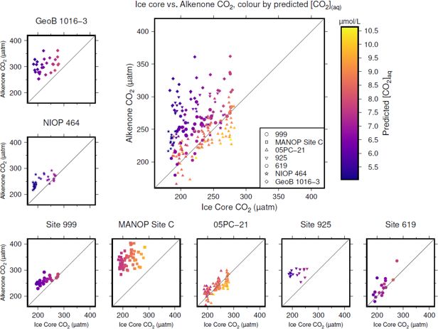
1152                                                                                 M. P. S. Badger: CCMs in coccolithophores at low CO2

Table 1. Sites with Pleistocene CO2(εp −alk) records. Note that the MANOP Site C record was generated to track changes in surface water–
atmosphere equilibrium, not atmospheric pCO2 , so, although it is included here for completeness, it is not included in the analysis. Distance
from the coast is calculated from the intermediate-resolution version of GSHHG and computed using Generic Mapping Tools (Wessel and
Smith, 1996; Wessel et al., 2019).

         Site                    Age interval       Latitude        Longitude             Water     Distance from     Reference
                                        (kyr)                                          depth (m)       coast (km)
         05PC-21                      0.5–188       38◦ 240 N       131◦ 330 E              1721               108    Bae et al. (2015)
         DSDP 619                        3–92       27◦ 11.610 N    91◦ 24.540 W            2259               489    Jasper and Hayes (1990)
         NIOP 464                      7.8–29       22◦ 90 N        63◦ 210 E               1470               333    Palmer et al. (2010)
         ODP 999                     111–258        12◦ 44.6390 N   78◦ 44.3600 W           2839               249    Badger et al. (2019)
         ODP 925                      20–580        4◦ 12.2490 N    43◦ 29.3340 W           3042               626    Zhang et al. (2013)
         MANOP Site C                0.8–253        0◦ 57.20 N      138◦ 57.30 W            4287               998    Jasper et al. (1994)
         GeoB 1016-3                 1.3–196        11◦ 46.20 S     11◦ 40.90 E             3410               185    Andersen et al. (1999)

       The full record for ODP Site 925 extends to 38.62 Ma.

Table 2. Sources of ice core data, as compiled by Bereiter et al. (2015). WAIS – West Antarctic Ice Sheet; TALDICE – TALos Dome Ice
CorE; and EDML – EPICA Dronning Maud Land. Age given as gas age relative to 1950.

                                         Age interval (kyr)    Ice core location     Reference
                                         −0.051 to 1.8         Law Dome              Rubino et al. (2013)
                                         1.8–2                 Law Dome              MacFarling Meure et al. (2006)
                                         2–11                  Dome C                Monnin et al. (2001, 2004)
                                         11–22                 WAIS                  Marcott et al. (2014)
                                         22–40                 Siple Dome            Ahn and Brook (2014)
                                         40–60                 TALDICE               Bereiter et al. (2012)
                                         60–115                EDML                  Bereiter et al. (2012)
                                         105–155               Dome C                Schneider et al. (2013)
                                         155–393               Vostok                Petit et al. (1999)

and                                                                                growth rate, and [PO3−  4 ] has recently been questioned (Zhang

                   εCO2(aq) −CO2(g)
                                                                                  et al., 2019, 2020) but for the purposes of this analysis is as-
δ 13 CCO2(aq)   =                   +1                                             sumed to hold. This is discussed further below. Values for
                        1000                                                       SST, δ 13 Calkenone , δ 13 Ccarbonate , salinity, and [PO3−
                                                                                                                                            4 ] are ei-
                                                                      (5)        ther taken from the original publications or estimated from
                  × δ 13 CCOc(g) + 1000
                                                                                   modern ocean estimates (Takahashi et al., 2009; Antonov
                  − 1000.                                                          et al., 2010; Garcia et al., 2013; Locarnini et al., 2013).
                                                                                      Providing that the atmosphere is in equilibrium with sur-
   Finally εp can be calculated:
                                                                                   face water, the concentration of atmospheric CO2 can be cal-
        δ 13 CCO2(aq) + 1000
                                !                                                  culated from [CO2 ](aq) (and vice versa if atmospheric CO2
εp =                         − 1 × 1000,                                (6)        concentration is known) using Henry’s law:
           δ 13 Corg + 1000
                                                                                             [CO2 ](aq)
and from that [CO2 ](aq) is calculated using the isotopic frac-                    pCO2 =               .                                          (8)
                                                                                               KH
tionation during carbon fixation (εf ) and b, which represents
the summation of physiological factors:                                               The solubility coefficient (KH ) is dependent on salinity
                                                                                   and SST, and here it is calculated following the parameter-
                    b
[CO2 ](aq) =             .                                              (7)        ization of Weiss (1970, 1974).
                 εf − εp

   Here εf is assumed to be a constant 25 ‰ (Bidigare et al.,
1997). In the modern ocean the b term, which accounts
for physiological factors such as cell size and growth rate,
shows a close correlation with [PO3−
                                   4 ] (Bidigare et al., 1997;
Pagani et al., 2009). However, the relationship between b,

Biogeosciences, 18, 1149–1160, 2021                                                                    https://doi.org/10.5194/bg-18-1149-2021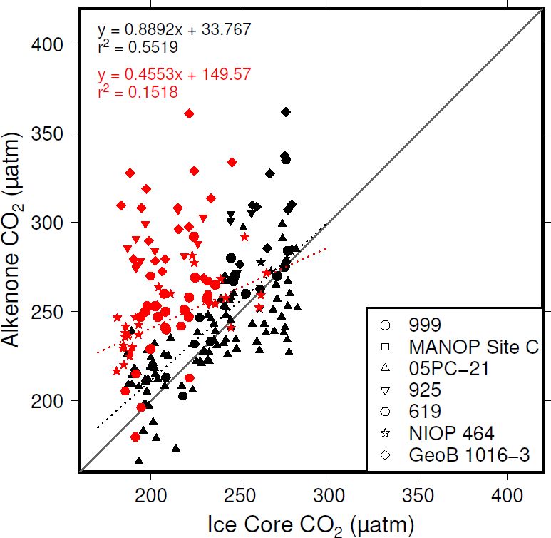
M. P. S. Badger: CCMs in coccolithophores at low CO2                                                                              1153

                                                                          To produce time-equivalent estimates of atmospheric CO2
                                                                       concentration for comparison with the ice core records, a
                                                                       simple linear interpolation of the Bereiter et al. (2015) com-
                                                                       pilation was initially used (Fig. 4). This assumes that both
                                                                       the age model of the ice core and the published age mod-
                                                                       els of the sites are correct and equivalent. This is almost
                                                                       certainly not the case, and so for the calculations below, a
                                                                       ±3000 year uncertainty is included for ages of both the ice
                                                                       core and CO2(εp −alk) values. Figure 4 shows that CO2(εp −alk) -
                                                                       based atmospheric CO2 concentration agree with ice core
Figure 3. Compiled CO2(εp −alk) -based estimates of atmospheric        CO2 at some sites and at some times, but not throughout.
CO2 concentration over the past 260 kyr (blue circles), with the ice   Sites 05-PC21 (Bae et al., 2015) and DSDP Site 619 (Jasper
core compilation of Bereiter et al. (2015) shown as the solid black    and Hayes, 1990) perform quite well throughout, whilst ODP
line. Full sources for the ice core and CO2(εp −alk) records are in    Site 999 (Badger et al., 2019) and NIOP 464 (Palmer et al.,
Tables 1 and 2.                                                        2010) only appear to agree at higher values of CO2 , and at
                                                                       ODP Site 925 (Zhang et al., 2013) and GeoB 1016-3 (Ander-
                                                                       sen et al., 1999) there is very little overlap between the two
3     Results
                                                                       methods of reconstructing atmospheric CO2 concentration.
3.1    Multi-site comparisons between CO2(εp −alk) and                    To explore whether [CO2 ](aq) is an important in-
       the ice core records                                            fluence on CO2(εp −alk) , I calculate predicted [CO2 ](aq)
                                                                       ([CO2 ](aq)−predicted ) for each of the samples. To calcu-
Across the six sites included in this analysis, there are 217          late [CO2 ](aq)−predicted , the time-equivalent value of atmo-
CO2(εp −alk) -based estimates of atmospheric CO2 concentra-            spheric CO2 concentration from the ice core record is
tion over the past 260 kyr for comparison with the ice core            used in combination with Eq. (8) to calculate [CO2 ](aq)
records (Table 2; Bereiter et al., 2015). When all CO2(εp −alk)        at the time of alkenone production for each sample. Re-
estimates are considered together over 260 kyr, this compi-            constructed estimates of SST and salinity are used as for
lation of proxy-based records fails to replicate the ice core          CO2(εp −alk) above, along with any estimated surface water–
record (Fig. 3). This has already been noted at specific sites         atmosphere disequilibrium. Points in Fig. 4 are then coloured
(e.g. Site 999 in the Caribbean; Badger et al., 2019), but             by [CO2 ](aq)−predicted .
this is the first time that all available records coincident with         Inspection of Fig. 4 suggests a connection between
the Pleistocene ice core records have been compiled using              ([CO2 ](aq)−predicted ) and the skill of CO2(εp −alk) to recon-
a common methodology. Notably the CO2(εp −alk) -based esti-            struct atmospheric CO2 concentration. The points clustering
mates are rarely lower than time-equivalent ice core estimate,         around the 1 : 1 line are lighter in colour (so with higher
but frequently higher. Given that haptophytes require carbon           [CO2 ](aq)−predicted ), whilst points falling away from the 1 :
to satisfy metabolic demand, this is perhaps unsurprising; if          1 line have lower [CO2 ](aq)−predicted . To explore this re-
at times of low carbon availability haptophytes can switch             lationship, I progressively restricted the included samples
from passive to active uptake to satisfy metabolic demand, it          on the basis of [CO2 ](aq)−predicted and at each stage calcu-
would be times of low atmospheric CO2 concentration (and               lated a Pearson correlation coefficient (r) and coefficient
so lower [CO2 ](aq) ) when the active uptake is most likely to         of determination (r 2 ) for each subset. Under this analysis
be needed. As CO2(εp −alk) -based estimates of atmospheric             the correlation progressively increased as more of the low
CO2 concentration rely on the assumption of a purely dif-              [CO2 ](aq)−predicted samples were excluded (Fig. 5). All anal-
fusive uptake of carbon, it is therefore likely that the proxy         yses were performed in R (R Core Team, 2020) using RStu-
would perform worse at times of low atmospheric CO2 con-               dio (RStudio Team, 2020). This suggests that the fidelity of
centration.                                                            the CO2(εp −alk) depends on the concentration of [CO2 ](aq) ,
   The haptophytes do not directly interact with the atmo-             improving at higher levels of [CO2 ](aq) .
sphere, obtaining their carbon from dissolved carbon. As it is            To further investigate this potential relationship, I progres-
not only atmospheric CO2 concentration which controls the              sively exclude samples based on [CO2 ](aq)−predicted with a
concentration of dissolved carbon ([CO2 ](aq) ) but also tem-          step size of 0.05 µmol L−1 , again calculating Pearson cor-
perature, alkalinity, and other oceanographic factors which            relation coefficients and coefficients of determination be-
control the equilibrium state between surface waters at the            tween ice core and CO2(εp −alk) for each subsample of the
atmosphere (Fig. 2), the multiple sites in different settings          population. The result is shown in Fig. 6. Here the analy-
now give the opportunity to test whether other factors are             sis shows, similar to Fig. 5, that, as the samples with low-
important in controlling the accuracy of CO2(εp −alk) .                est [CO2 ](aq)−predicted are progressively removed, the corre-
                                                                       lation between ice core and CO2(εp −alk) increases. Further-
                                                                       more, this continues only up until [CO2 ](aq)−predicted reaches

https://doi.org/10.5194/bg-18-1149-2021                                                       Biogeosciences, 18, 1149–1160, 2021
1154 M. P. S. Badger: CCMs in coccolithophores at low CO2
Figure 4. Crossplots of CO2(εp −alk) -based atmospheric CO2 concentration (y axes) vs. the time-equivalent estimate from ice core records
(x axes; Bereiter et al., 2015; Table 2). The large panel compiles all sites, with the exception of MANOP Site C, as explained in the text.
Symbols are coloured by predicted [CO2 ](aq) for each site and time as explained in the text. Full sources for alkenone data are shown in
Table 1. A 1 : 1 line is included in all plots for comparison.
7 µmol L−1 . Above this, the coefficient of determination pling of the ice core record, and it is applied as a normally
plateaus, until the subsample reaches such a small size that distributed uncertainty. Uncertainty in CO2(εp −alk) measure-
spurious correlations become important (Fig. 6b). ments is typically calculated using Monte Carlo modelling
of all the parameters (i.e. Pagani et al., 1999; Badger et al.,
3.2 Sensitivity and uncertainty tests 2013a, b); however this was not done in all the published
work (Table 1), and some differences in approach were found
It is possible that the pattern seen in Fig. 6b could emerge across the published work. Therefore to create CO2(εp −alk)
from a dataset shaped with increasing density surrounding uncertainty estimates for each value in this study, I emu-
the 1 : 1 correlation line without being driven by changes in late the uncertainties based on the CO2(εp −alk) value. I built
[CO2 ](aq)−predicted . To explore this possibility, I ran a series a simple emulator (Fig. 7) by running Monte Carlo uncer-
of sensitivity experiments. In these, rather than reducing the tainty estimates for all of the included datasets (Table 1)
sample by filtering by [CO2 ](aq)−predicted , the whole dataset using the same estimates of uncertainty for each variable
(Table 1) was randomly ordered and then stepwise subsam- in the CO2(εp −alk) calculation as applied in Badger et al.
pled. To make this equivalent to the [CO2 ](aq)−predicted anal- (2013a, b). This then allows the uncertainty to be included in
ysis above, I set the size of each subsample to be equal to the [CO2 ](aq)−predicted calculation as well as CO2(εp −alk) , and
each step in the original analysis. This produces a randomly it allowed for uncertainty estimates to be site-ambivalent.
selected but same-sized subsample such that the size of the The result is shown in Fig. 6c and d, and it suggests that
subsample reduces in the same way as shown in Fig. 6b). the 7 µmol L−1 break point remains valid. The absolute value
Pearson correlation coefficients and coefficients of determi- of r 2 is reduced, even at higher [CO2 ](aq)−predicted , but this
nation were calculated for each subsample as above, and I would be expected given the addition of uncertainty in the
repeated this 1000 times, with the order of each sample ran- age model, as the published age is most likely to align with
domized each time. the ice core. Given the rapid rate of change at deglacia-
To allow for possible age model uncertainties, a 3000-year tions, this effect is likely to be particularly pronounced in
(1σ ) uncertainty was also applied to each sample. This un- this dataset as many records have high temporal resolution
certainty was applied to the age of each sample prior to sam- around deglaciations in order to attempt to resolve them.
Biogeosciences, 18, 1149–1160, 2021 https://doi.org/10.5194/bg-18-1149-2021M. P. S. Badger: CCMs in coccolithophores at low CO2 1155
Figure 5. Crossplots of CO2(εp −alk) -based atmospheric CO2 concentration (Table 1; y axes) vs. the time-equivalent estimate from ice
core records (x axes; Bereiter et al., 2015; Table 2). The sample of published vales of CO2(εp −alk) was progressively restricted by
[CO2 ](aq)−predicted , indicated by the subplot titles. Individual values are coloured by [CO2 ](aq)−predicted , and sites indicated by shape
(see key). Coefficients of determination and equations of best fit are shown in each panel, along with a 1 : 1 line.
Any small age model offset introduced by the error mod- some culture studies (Laws et al., 1997, 2002; Cassar et al.,
elling in these intervals also clearly has the potential to in- 2006), with some evidence that the diatom Phaeodactylum
duce large differences between the CO2(εp −alk) and ice core tricornutum has a similar CCM threshold of 7 µmol L−1
values. Figure 6c and d clearly demonstrate that it is the fil- (Laws et al., 1997). Whilst the evidence for the mechanism
tering by [CO2 ](aq)−predicted rather than any spurious correla- of CCM is poorer for coccolithophores than it is for diatoms,
tions which determines the shape of the data in Fig. 6a. any CCM would be expected to compromise the CO2(εp −alk)
proxy, either by increased supply of [CO2 ](aq) or by further
carbon isotopic fractionation effects during carbon transport,
4 Discussion or both (Stoll et al., 2019).
By applying a threshold value for [CO2 ](aq)−predicted of
The plateau in r 2 in Fig. 6a and c suggests that be- 7 µmol L−1 to the published records (Table 1), values of
low a [CO2 ](aq)−predicted of ∼ 7 µmol L−1 CO2(εp −alk) CO2(εp −alk) which are influenced by active CCMs can be
is no longer as good a predictor of ice core CO2 as eliminated. Recognition of this new threshold value of
when [CO2 ](aq)−predicted > 7 µmol L−1 . This is clear [CO2 ](aq)−predicted allows for a new record of Pleistocene
from comparing the relationship between samples CO2(εp −alk) to be compiled. This compilation then much bet-
where [CO2 ](aq)−predicted < 7 µmol L−1 with those where ter replicates the glacial–interglacial pattern of CO2 change
[CO2 ](aq)−predicted > 7 µmol L−1 in Fig. 8. Here the r 2 for over the last 260 kyr (Fig. 9). Whilst this present com-
the former of 0.15 is substantially less than the latter of pilation does rely on ice core CO2 records to estimate
0.55. I suggest that this is because below this threshold [CO2 ](aq)−predicted , and therefore has little direct utility as
the fundamental assumption of CO2(εp −alk) , that carbon is a CO2 record, it does demonstrate that recognition of a
passively taken up by haptophytes, no longer holds true. threshold response allows accurate CO2 reconstruction us-
One obvious explanation for why this would be the case is ing CO2(εp −alk) . This may represent the point at which iso-
that at low levels of [CO2 ](aq) haptophytes have to rely more topic effects of CCMs (plausibly through increased CA ac-
on active uptake of carbon via CCMs in order to satisfy tivity or HCO− 3 dehydration to meet C demand) overwhelm
metabolic demand. Similar behaviour has been recognized in the assumptions of the CO2(εp −alk) proxy. This, as well as
https://doi.org/10.5194/bg-18-1149-2021 Biogeosciences, 18, 1149–1160, 20211156 M. P. S. Badger: CCMs in coccolithophores at low CO2
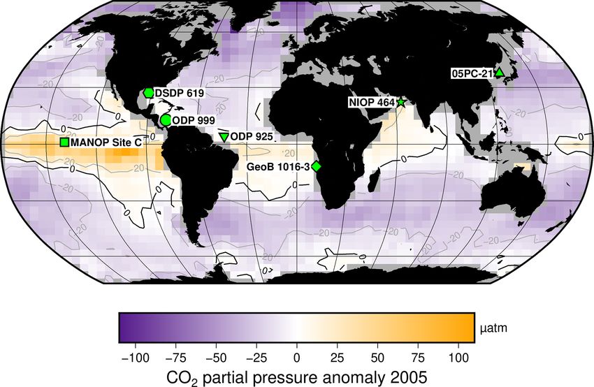
Figure 6. Coefficient of determination (a) of a reducing sample of all compiled CO2(εp −alk) (Table 1) vs. the time-equivalent estimate from
ice core records (Bereiter et al., 2015; Table 2). The sample reduces stepwise by 0.05 µmol L−1 , and the number of records in each subsample
is shown in panel (b). Panel (c) shows a 1000-member Monte Carlo analysis, whereby uncertainty in CO2(εp −alk) and age is considered,
as detailed in the text. Panel (d) shows a similar 1000-member Monte Carlo analysis, but with random sampling of the whole CO2(εp −alk)
population so that the number of samples is equivalent to the dataset shown in panel (c); i.e. the size of the sample follows that shown in
panel (b). Means and 1σ uncertainties are shown as the bold lines.
Figure 8. Correlations between CO2(εp −alk) and ice core CO2 ,
Figure 7. Emulated uncertainty in CO2(εp −alk) , generated by run-
ning Monte Carlo uncertainty models for all sites in Table 1, apply- where [CO2 ](aq)−predicted > 7 µmol L−1 (black symbols) and
ing the same approach to uncertainty as Badger et al. (2013a, b). [CO2 ](aq)−predicted < 7 µmol L−1 (red symbols).
Estimates used in this study are highlighted in blue.
areas of the ocean (or intervals of time) with low [CO2 ](aq)
the behaviour shown in Fig. 6a and c, suggests that from the can be avoided, accurate reconstructions of atmospheric CO2
standpoint of the CO2(εp −alk) proxy CCMs may effectively concentration can be acquired using CO2(εp −alk) .
be considered either active or not, and that when [CO2 ](aq) As [CO2 ](aq) is affected by both SST via the tempera-
is plentiful passive uptake dominates, at least sufficiently in ture dependance of the Henry’s law constant and atmospheric
most oceanographic settings that CO2(εp −alk) can accurately CO2 concentration, for CO2(εp −alk) to be effective in recon-
record atmospheric CO2 concentration. This implies that, if structing atmospheric CO2 concentration, areas of warm wa-
Biogeosciences, 18, 1149–1160, 2021 https://doi.org/10.5194/bg-18-1149-2021M. P. S. Badger: CCMs in coccolithophores at low CO2 1157
of passive carbon uptake inherent in CO2(εp −alk) as tradition-
ally applied may still be valid.
5 Conclusions
Reconstructions of past atmospheric CO2 concentration with
proxy tools like CO2(εp −alk) are critical for understanding
how the Earth’s climate system operates, as long as the tools
used can be relied upon to be accurate and precise. This re-
analysis of existing Pleistocene CO2(εp −alk) records reveals
that below a critical threshold of [CO2 ](aq) of 7 µmol−1 the
Figure 9. Revised compilation of Pleistocene CO2(εp −alk) vs. ice relationship between δ 13 Calkenone and atmospheric CO2 con-
core records. The compiled published records (Table 1) are shown centration breaks down, plausibly because below this thresh-
as circles, coloured red where [CO2 ](aq)−predicted is below a thresh- old haptophytes are able to actively take up carbon using
old of 7 µmol−1 and blue where [CO2 ](aq)−predicted > 7 µmol−1 . CCMs in order to satisfy metabolic demand.
The solid blue line is a loess filter (span 0.1) through the Although reconstructing the low levels of atmospheric
[CO2 ](aq)−predicted > 7 µmol−1 values, with 95 % confidence inter- CO2 concentration in the Pleistocene glacials and areas of
vals (dashed blue line). The black line is the ice core compilation of the global ocean where [CO2 ](aq) is less than 7 µmol−1 will
Bereiter et al. (2015) (Table 2). be impossible, for much of the Cenozoic the CO2(εp −alk)
proxy retains utility. If care is taken to avoid regions and
oceanographic settings where [CO2 ](aq) is expected to be ab-
ter (i.e. tropical or shallow shelf regions) under relatively low normally low, CO2(εp −alk) remains an important and useful
atmospheric CO2 concentration must be avoided. However, proxy to understand the Earth system.
as the atmospheric CO2 control renders the global surface
ocean sufficiently replete with [CO2 ](aq) at Pliocene-like lev-
Code and data availability. This paper relies exclusively on previ-
els of atmospheric CO2 concentration and above (Martínez-
ously published data, available with the original papers and in pub-
Botí et al., 2015) at all but the warmest surface ocean temper- licly available repositories. An R notebook supplement is available
atures, CO2(εp −alk) is likely to be a reliable system for most alongside this paper, along with data files, which allow full replica-
of the Cenozoic. It is only in the Pleistocene that atmospheric tion of all analyses performed.
CO2 concentration is low enough for CCMs to be widely
active across the surface ocean, with the low-CO2 glacials
providing the most difficulty (Badger et al., 2019). This find- Supplement. The supplement related to this article is available on-
ing aligns well with evidence that CCMs developed in coc- line at: https://doi.org/10.5194/bg-18-1149-2021-supplement.
colithophores as a response to declining atmospheric CO2
concentration through the Cenozoic and were developing in
[CO2 ](aq) -limited parts of the ocean in the late Miocene at the Competing interests. The author declares that there is no conflict of
earliest, and likely not widespread until the Plio-Pleistocene interest.
(Bolton et al., 2012; Bolton and Stoll, 2013).
There have been recent attempts to correct for CCMs in
CO2(εp −alk) -based reconstructions of atmospheric CO2 con- Acknowledgements. I am grateful to Gavin Foster and Tom Chalk
centrations (Zhang et al., 2019; Stoll et al., 2019; Zhang for frequent and stimulating discussions on alkenone paleaobarom-
et al., 2020). However, these assume that CCMs are al- etry. I thank all authors who made full datasets available online.
I thank Kirsty Edgar for comments on various drafts and the two
ways active and crucially do not fundamentally break the
anonymous reviewers, whose comments greatly improved this pa-
relationship between εp values and atmospheric CO2 con- per.
centration. However if this is not the case, and the rela-
tionship between εp values and atmospheric CO2 concen-
tration fails at Pleistocene levels of atmospheric CO2 , then Financial support. Financial support for this work was provided
Pleistocene records cannot be used to develop corrections of by the School of Environment, Earth and Ecosystem Sciences, The
CO2(εp −alk) to be applied throughout the Cenozoic. If, as sug- Open University.
gested by the analyses presented here, CCMs only act at low
[CO2 ](aq) , and largely only in conditions prevalent through-
out the late Pliocene and Pleistocene, it is plausible that cor- Review statement. This paper was edited by Jack Middelburg and
rections based on Pleistocene records could overcompensate reviewed by two anonymous referees.
for CCMs in the rest of the Cenozoic, when the assumption
https://doi.org/10.5194/bg-18-1149-2021 Biogeosciences, 18, 1149–1160, 20211158 M. P. S. Badger: CCMs in coccolithophores at low CO2
References Bolton, C. T. and Stoll, H. M.: Late Miocene threshold response of
marine algae to carbon dioxide limitation, Nature, 500, 558–562,
https://doi.org/10.1038/nature12448, 2013.
Ahn, J. and Brook, E. J.: Siple Dome ice reveals two modes of mil- Bolton, C. T., Stoll, H. M., and Mendez-Vicente, A.: Vital effects in
lennial CO2 change during the last ice age, Nat. Commun., 5, coccolith calcite: Cenozoic climate-pCO2 drove the diversity of
3723, https://doi.org/10.1038/ncomms4723, 2014. carbon acquisition strategies in coccolithophores?, Paleoceanog-
Anagnostou, E., John, E. H., Edgar, K. M., Foster, G. L., Ridg- raphy, 27, PA4204, https://doi.org/10.1029/2012PA002339,
well, A., Inglis, G. N., Pancost, R. D., Lunt, D. J., and Pear- 2012.
son, P. N.: Changing atmospheric CO2 concentration was the Brassell, S., Eglinton, G., and Marlowe, I.: Molecular stratigraphy:
primary driver of early Cenozoic climate, Nature, 533, 380–384, a new tool for climatic assessment, Nature, 320, 129–133, 1986.
https://doi.org/10.1038/nature17423, 2016. Cassar, N., Laws, E. A., and Popp, B. N.: Carbon iso-
Andersen, N., Müller, P. J., Kirst, G., and Schneider, R. R.: topic fractionation by the marine diatom Phaeodacty-
Alkenone δ 13 C as a Proxy for PastP CO2 in Surface Waters: lum tricornutum under nutrient- and light-limited growth
Results from the Late Quaternary Angola Current, in: Use conditions, Geochim. Cosmochim. Ac., 70, 5323–5335,
of Proxies in Paleoceanography, edited by: Fischer, G., and https://doi.org/10.1016/j.gca.2006.08.024, 2006.
Wefer, G., Springer, Heidelberg, Berlin, Germany, 469–488, Conte, M. H., Volkman, J. K., and Eglinton, G.: Lipid biomarkers
https://doi.org/10.1007/978-3-642-58646-0_19, 1999. of the Haptophyta, in: The Haptophyte algae, edited by: Green, J.
Antonov, J. I., Seidov, D., Boyer, T. P., Locarnini, R. A., Mishonov, and Leadbeater, B., Oxford University Press, Oxford, UK, 351–
A. V., Garcia, H. E., Baranova, O. K., Zweng, M. M., and John- 377, 1994.
son, D. R.: World Ocean Atlas 2009, Salinity, vol. 2, edited by: Farrimond, P., Eglinton, G., and Brassell, S. C.: Alkenones
Levitus, S., US Government Printing Office, Washington DC, in Cretaceous black shales, Blake-Bahama Basin, west-
USA, NOAA Atlas NESDIS 69, 184 pp., 2010. ern North Atlantic, Org. Geochem., 10, 897–903,
Badger, M. P. S., Lear, C. H., Pancost, R. D., Foster, G. L., Bailey, https://doi.org/10.1016/S0146-6380(86)80027-4, 1986.
T. R., Leng, M. J., and Abels, H. A.: CO2 drawdown following Foster, G. L., Lear, C. H., and Rae, J. W. B.: The evo-
the middle Miocene expansion of the Antarctic Ice Sheet, Pa- lution of pCO2 , ice volume and climate during the mid-
leoceanography, 28, 42–53, https://doi.org/10.1002/palo.20015, dle Miocene, Earth Planet. Sc. Lett., 341–344, 243–254,
2013a. https://doi.org/10.1016/j.epsl.2012.06.007, 2012.
Badger, M. P. S., Schmidt, D. N., Mackensen, A., and Foster, G. L., Royer, D. L., and Lunt, D. J.: Future climate forc-
Pancost, R. D.: High-resolution alkenone palaeobarome- ing potentially without precedent in the last 420 million years,
try indicates relatively stable pCO2 during the Pliocene Nat. Commun., 8, 14845, https://doi.org/10.1038/ncomms14845,
(3.3–2.8 Ma), Philos. T. Roy. Soc. A, 371, 20130094, 2017.
https://doi.org/10.1098/rsta.2013.0094, 2013b. Garcia, H. E., Locarnini, R. A., Boyer, T. P., Antonov, J. I., Bara-
Badger, M. P. S., Chalk, T. B., Foster, G. L., Bown, P. R., Gibbs, nova, O. K., Zweng, M. M., Reagan, J. R., and Johnson, D. R.:
S. J., Sexton, P. F., Schmidt, D. N., Pälike, H., Mackensen, A., World Ocean Atlas 2013, Dissolved Inorganic Nutrients (phos-
and Pancost, R. D.: Insensitivity of alkenone carbon isotopes to phate, nitrate, silicate), vol. 4, edited by: Levitus, S. and Mis-
atmospheric CO2 at low to moderate CO2 levels, Clim. Past, 15, honov, A., Tech. Rep., NOAA Atlas NESDIS 76, 25 pp., Silver
539–554, https://doi.org/10.5194/cp-15-539-2019, 2019. Spring, MD, USA, 2014.
Bae, S. W., Lee, K. E., and Kim, K.: Use of carbon Gradstein, F., Ogg, J., Schmitz, M., and Ogg, G.: The Ge-
isotopic composition of alkenone as a CO2 proxy in ologic Time Scale 2012, 1st Edn., Elsevier, 1176 pp.,
the East Sea/Japan Sea, Cont. Shelf Res., 107, 24–32, https://doi.org/10.1016/C2011-1-08249-8, 2012.
https://doi.org/10.1016/j.csr.2015.07.010, 2015. Jasper, J. and Hayes, J.: A carbon isotope record of CO2 levels dur-
Beerling, D. J. and Royer, D. L.: Convergent Cenozoic CO2 history, ing the late Quaternary, Nature, 347, 462–464, 1990.
Nat. Geosci., 4, 418–420, https://doi.org/10.1038/ngeo1186, Jasper, J., Hayes, J., Mix, A., and Prahl, F.: Photosynthetic fraction-
2011. ation of 13 C and concentrations of dissolved CO2 in the central
Bereiter, B., Lüthi, D., Siegrist, M., Schüpbach, S., Stocker, T. F., equatorial Pacific during the last 255 000 years, Paleoceanogra-
and Fischer, H.: Mode change of millennial CO2 variability phy, 9, 781–798, 1994.
during the last glacial cycle associated with a bipolar ma- Kürschner, W. M., Kvacek, Z., and Dilcher, D. L.: The impact of
rine carbon seesaw, P. Natl. Acad. Sci. USA, 109, 9755–9760, Miocene atmospheric carbon dioxide fluctuations on climate and
https://doi.org/10.1073/pnas.1204069109, 2012. the evolution, P. Natl. Acad. Sci. USA, 105, 449–453, 2008.
Bereiter, B., Eggleston, S., Schmitt, J., Nehrbass-Ahles, C., Laws, E. A., Popp, B., Bidigare, R., Kennicutt, M., and Macko, S.:
Stocker, T. F., Fischer, H., Kipfstuhl, S., and Chappellaz, Dependence of phytoplankton carbon isotopic composition on
J.: Revision of the EPICA Dome C CO2 record from 800 growth rate and [CO2 ) aq: Theoretical considerations and exper-
to 600 kyr before present, Geophys. Res. Lett., 42, 542–549, imental, Geochim. Cosmochim. Ac., 59, 1131–1138, 1995.
https://doi.org/10.1002/2014GL061957, 2015. Laws, E. A., Bidigare, R. R., and Popp, B. N.: Effect of growth rate
Bidigare, R., Fluegge, A., Freeman, K. H., Hanson, K., Hayes, J. M., and CO2 concentration on carbon isotopic fractionation by the
Hollander, D., Jasper, J. P., King, L. L., Laws, E. A., Milder, J., marine diatom Phaeodactylum tricornutum, Limnol. Oceanogr.,
Millero, F. J., Pancost, R., Popp, B. N., Steinberg, P., and Wake- 42, 1552–1560, https://doi.org/10.4319/lo.1997.42.7.1552,
ham, S. G.: Consistent fractionation of 13 C in nature and in the 1997.
laboratory: Growth-rate effects in some haptophyte algae, Global
Biochem. Cy., 11, 279–292, 1997.
Biogeosciences, 18, 1149–1160, 2021 https://doi.org/10.5194/bg-18-1149-2021M. P. S. Badger: CCMs in coccolithophores at low CO2 1159
Laws, E. A., Popp, B. N., Cassar, N., and Tanimoto, J.: 13 C carbon dioxide concentrations, Nat. Geosci., 3, 27–30,
discrimination patterns in oceanic phytoplankton: likely in- https://doi.org/10.1038/ngeo724, 2009.
fluence of CO2 concentrating mechanisms, and implications Pagani, M., Huber, M., Liu, Z., Bohaty, S. M., Henderiks, J., Sijp,
for palaeoreconstructions, Funct. Plant Biol., 29, 323–333, W., Krishnan, S., and De Conto, R. M.: The role of carbon diox-
https://doi.org/10.1071/Pp01183, 2002. ide during the onset of Antarctic glaciation, Science, 334, 1261–
Locarnini, R. A., Mishonov, A. V., Antonov, J. I., Boyer, T. P., 1264, https://doi.org/10.1126/science.1203909, 2011.
Garcia, H. E., Baranova, O. K., Zweng, M. M., Paver, C. R., Palmer, M. R., Brummer, G. J., Cooper, M. J., Elderfield, H.,
Reagan, J. R., Johnson, D. R., Hamilton, M., and Seidov, D.: Greaves, M. J., Reichart, G. J., Schouten, S., and Yu, J. M.:
World Ocean Atlas 2013, Temperature, vol. 1, edited by: Lev- Multi-proxy reconstruction of surface water pCO2 in the north-
itus, S. and Mishonov, A., Tech. Rep., NOAA Atlas NES- ern Arabian Sea since 29 ka, Earth Planet. Sc. Lett., 295, 49–57,
DIS 73, 40 pp., Silver Springs, MD, USA, available at: https: https://doi.org/10.1016/j.epsl.2010.03.023, 2010.
//www.nodc.noaa.gov/OC5/woa13/pubwoa13.html (last access: Pearson, P. N., Foster, G. L., and Wade, B. S.: Atmospheric car-
12 February 2021), 2013. bon dioxide through the Eocene-Oligocene climate transition,
MacFarling Meure, C., Etheridge, D., Trudinger, C., Steele, P., Nature, 461, 1110–1113, https://doi.org/10.1038/nature08447,
Langenfelds, R., van Ommen, T., Smith, A., and Elkins, 2009.
J.: Law Dome CO2 , CH4 and N2 O ice core records ex- Petit, J. R., Jouzel, J., Raynaud, D., Barkov, N. I., Barnola, J.-M.,
tended to 2000 years BP, Geophys. Res. Lett., 33, L14810, Basile, I., Bender, M., Chappellaz, J., Davis, M., Delaygue, G.,
https://doi.org/10.1029/2006gl026152, 2006. Delmotte, M., Kotlyakov, V. M., Legrand, M., Lipenkov, V. Y.,
Marcott, S. A., Bauska, T. K., Buizert, C., Steig, E. J., Rosen, J. L., Lorius, C., Pepin, K., Ritz, C., Saltzman, E., and Stievenard, M.:
Cuffey, K. M., Fudge, T. J., Severinghaus, J. P., Ahn, J., Kalk, Climate and atmospheric history of the past 420 000 years from
M. L., McConnell, J. R., Sowers, T., Taylor, K. C., White, J. the Vostok ice core, Antarctica, Nature, 399, 429–436, 1999.
W. C., and Brook, E. J.: Centennial-scale changes in the global Popp, B., Laws, E. A., Bidigare, R., Dore, J., Hanson, K., and Wake-
carbon cycle during the last deglaciation, Nature, 514, 616–619, ham, S. G.: Effect of phytoplankton cell geometry on carbon iso-
2014. topic fractionation, Geochim. Cosmochim. Ac., 62, 67–77, 1998.
Marlowe, I., Brassell, S., Eglinton, G., and Green, J.: Long- R Core Team: A language and environment for statistical comput-
chain alkenones and alkyl alkenoates and the fossil coccol- ing, available at: https://www.r-project.org/ (last access: 9 Octo-
ith record of marine sediments, Chem. Geol., 88, 349–375, ber 2020), 2020.
https://doi.org/10.1016/0009-2541(90)90098-R, 1990. R Studio Team: Integrated Development for R, RStudio, PBC,
Martínez-Botí, M. A., Foster, G. L., Chalk, T. B., Rohling, E. J., Boston, MA, USA, available at: http://www.rstudio.com/, last ac-
Sexton, P. F., Lunt, D. J., Pancost, R. D., Badger, M. P. S., cess: 18 September 2020.
and Schmidt, D. N.: Plio-Pleistocene climate sensitivity eval- Raffi, I., Backman, J., Fornaciari, E., Pälike, H., Rio, D.,
uated using high-resolution CO2 records, Nature, 518, 49–54, Lourens, L., and Hilgen, F.: A review of calcareous
https://doi.org/10.1038/nature14145, 2015. nannofossil astrobiochronology encompassing the past
Monnin, E., Indermuhle, A., Dallenbach, A., Fluckiger, J., Stauffer, 25 million years, Quaternary Sci. Rev., 25, 3113–3137,
B., Stocker, T. F., Raynaud, D., and Barnola, J. M.: Atmospheric https://doi.org/10.1016/j.quascirev.2006.07.007, 2006.
CO2 concentrations over the last glacial termination, Science, Rechka, J. and Maxwell, J.: Characterisation of alkenone tempera-
291, 112–114, https://doi.org/10.1126/science.291.5501.112, ture indicators in sediments and organisms, Org. Geochem., 13,
2001. 727–734, 1987.
Monnin, E., Steig, E. J., Siegenthaler, U., Kawamura, K., Schwan- Reinfelder, J. R.: Carbon concentrating mechanisms in eukary-
der, J., Stauffer, B., Stocker, T. F., Morse, D. L., Barnola, J.- otic marine phytoplankton, Annu. Rev. Mar. Sci., 3, 291–315,
M., Bellier, B., Raynaud, D., and Fischer, H.: Evidence for sub- https://doi.org/10.1146/annurev-marine-120709-142720, 2011.
stantial accumulation rate variability in Antarctica during the Riebesell, U., Revill, A. T., Holdsworth, D. G., and Volk-
Holocene, through synchronization of CO2 in the Taylor Dome, man, J. K.: The effects of varying CO2 concentration on
Dome C and DML ice cores, Earth Planet. Sc. Lett., 224, 45–54, lipid composition and carbon isotope fractionation in Emil-
https://doi.org/10.1016/j.epsl.2004.05.007, 2004. iania huxleyi, Geochim. Cosmochim. Ac., 64, 4179–4192,
Mook, W. G., Bommerson, J. C., and Staverman, W. H.: Car- https://doi.org/10.1016/S0016-7037(00)00474-9, 2000.
bon isotope fractionation between dissolved bicarbonate and Riebesell, U., Schulz, K. G., Bellerby, R. G., Botros, M.,
gaseous carbon dioxide, Earth Planet. Sc. Lett., 22, 169–176, Fritsche, P., Meyerhöfer, M., Neill, C., Nondal, G., Oschlies,
https://doi.org/10.1016/0012-821X(74)90078-8, 1974. A., Wohlers, J., and Zöllner, E.: Enhanced biological carbon
Pagani, M., Freeman, K., and Arthur, M.: Late Miocene atmo- consumption in a high CO2 ocean, Nature, 450, 545–548,
spheric CO2 concentrations and the expansion of C4 grasses, https://doi.org/10.1038/nature06267, 2007.
Science, 285, 876–879, 1999. Romanek, C. S., Grossman, E. L., and Morse, J. W.: Carbon isotopic
Pagani, M., Zachos, J. C., Freeman, K. H., Tipple, B., and fractionation in synthetic aragonite and calcite: Effects of tem-
Bohaty, S.: Marked decline in atmospheric carbon dioxide perature and precipitation rate, Geochim. Cosmochim. Ac., 56,
concentrations during the Paleogene, Science, 309, 600–603, 419–430, https://doi.org/10.1016/0016-7037(92)90142-6, 1992.
https://doi.org/10.1126/science.1110063, 2005. Rost, B., Riebesell, U., Burkhardt, S., and Sülte-
Pagani, M., Liu, Z., La Riviere, J., and Ravelo, A. C.: High meyer, D.: Carbon acquisition of bloom-forming ma-
Earth-system climate sensitivity determined from Pliocene rine phytoplankton, Limnol. Oceanogr., 48, 55–67,
https://doi.org/10.4319/lo.2003.48.1.0055, 2003.
https://doi.org/10.5194/bg-18-1149-2021 Biogeosciences, 18, 1149–1160, 20211160 M. P. S. Badger: CCMs in coccolithophores at low CO2 Rubino, M., Etheridge, D. M., Trudinger, C. M., Allison, C. E., Bat- Tchernov, D., Silverman, J., Luz, B., Reinhold, L., and Ka- tle, M. O., Langenfelds, R. L., Steele, L. P., Curran, M., Bender, plan, A.: Massive light-dependent cycling of inorganic M., White, J. W. C., Jenk, T. M., Blunier, T., and Francey, R. J.: carbon between oxygenic photosynthetic microorganisms A revised 1000 year atmospheric δ 13 C-CO2 record from Law and their surroundings, Photosynth. Res., 77, 95–103, Dome and South Pole, Antarctica, J. Geophys. Res.-Atmos., 118, https://doi.org/10.1023/A:1025869600935, 2003. 8482–8499, https://doi.org/10.1002/jgrd.50668, 2013. Trimborn, S., Langer, G., and Rost, B.: Effect of varying calcium Schneider, R., Schmitt, J., Köhler, P., Joos, F., and Fischer, H.: concentrations and light intensities on calcification and photo- A reconstruction of atmospheric carbon dioxide and its stable synthesis in Emiliania huxleyi, Limnol. Oceanogr., 52, 2285– carbon isotopic composition from the penultimate glacial max- 2293, https://doi.org/10.4319/lo.2007.52.5.2285, 2007. imum to the last glacial inception, Clim. Past, 9, 2507–2523, Volkman, J. K.: Ecological and environmental fac- https://doi.org/10.5194/cp-9-2507-2013, 2013. tors affecting alkenone distributions in seawater Sosdian, S. M., Greenop, R., Hain, M. P., Foster, G. L., and sediments, Geochem. Geophy. Geosy., 1, 1036, Pearson, P. N., and Lear, C. H.: Constraining the evolu- https://doi.org/10.1029/2000GC000061, 2000. tion of Neogene ocean carbonate chemistry using the boron Weiss, R. F.: The solubility of nitrogen, oxygen and argon isotope pH proxy, Earth Planet. Sc. Lett., 498, 362–376, in water and seawater, Deep-Sea Res. Pt. I, 17, 721–735, https://doi.org/10.1016/j.epsl.2018.06.017, 2018. https://doi.org/10.1016/0011-7471(70)90037-9, 1970. Stoll, H. M., Guitian, J., Hernandez-Almeida, I., Mejia, L. M., Weiss, R. F.: Carbon dioxide in water and seawater: the solubility Phelps, S., Polissar, P., Rosenthal, Y., Zhang, H., and Ziveri, of a non-ideal gas, Mar. Chem., 2, 203–215, 1974. P.: Upregulation of phytoplankton carbon concentrating mecha- Wessel, P. and Smith, W. H. F.: A global, self-consistent, hierar- nisms during low CO2 glacial periods and implications for the chical, high-resolution shoreline database, J. Geophys. Res.-Sol. phytoplankton pCO2 proxy, Quaternary Sci. Rev., 208, 1–20, Ea., 101, 8741–8743, https://doi.org/10.1029/96JB00104, 1996. https://doi.org/10.1016/j.quascirev.2019.01.012, 2019. Wessel, P., Luis, J. F., Uieda, L., Scharroo, R., Wobbe, F., Super, J. R., Thomas, E., Pagani, M., Huber, M., Brien, C. O., Smith, W. H. F., and Tian, D.: The Generic Mapping and Hull, P. M.: North Atlantic temperature and pCO2 cou- Tools Version 6, Geochem. Geophy. Geosy., 20, 5556–5564, pling in the early-middle Miocene, Geology, 46, 519–522, https://doi.org/10.1029/2019GC008515, 2019. https://doi.org/10.1130/G40228.1, 2018. Zhang, Y. G., Pagani, M., Liu, Z., Bohaty, S. M., and Deconto, R.: Takahashi, T., Sutherland, S. C., Wanninkhof, R., Sweeney, C., A 40 million year history of atmospheric CO2 , Philos. T. Roy. Feely, R. A., Chipman, D. W., Hales, B., Friederich, G., Chavez, Soc. A, 371, 20130096, https://doi.org/10.1098/rsta.2013.0096, F., Sabine, C., Watson, A., Bakker, D. C. E., Schuster, U., Metzl, 2013. N., Yoshikawa-Inoue, H., Ishii, M., Midorikawa, T., Nojiri, Y., Zhang, Y. G., Pearson, A., Benthien, A., Dong, L., Huy- Körtzinger, A., Steinhoff, T., Hoppema, M., Olafsson, J., Arnar- bers, P., Liu, X., and Pagani, M.: Refining the alkenone- son, T. S., Tilbrook, B., Johannessen, T., Olsen, A., Bellerby, R., pCO2 method I: Lessons from the Quaternary glacial Wong, C. S., Delille, B., Bates, N. R., and de Baar, H. J. W.: Cli- cycles, Geochim. Cosmochim. Ac., 260, 177–191, matological mean and decadal change in surface ocean pCO2 , https://doi.org/10.1016/j.gca.2019.06.032, 2019. and net sea–air CO2 flux over the global oceans, Deep-Sea Res. Zhang, Y. G., Henderiks, J., and Liu, X.: Refining the alkenone- Pt. II, 56, 554–577, https://doi.org/10.1016/j.dsr2.2008.12.009, pCO2 method II: Towards resolving the physiological pa- 2009. rameter “b”, Geochim. Cosmochim. Ac., 281, 118–134, Takahashi, T., Sutherland, S. C., Chipman, D. W., Goddard, J., https://doi.org/10.1016/j.gca.2020.05.002, 2020. Newberber, T., and Sweeney, C.: Climatological Distributions Zondervan, I., Rost, B., and Riebesell, U.: Effect of CO2 con- of pH, pCO2 , Total CO2 , Alkalinity, and CaCO3 Saturation in centration on the PIC/POC ratio in the coccolithophore Emil- the Global Surface Ocean, Carbon Dioxide Information Analy- iania huxleyi grown under light-limiting conditions and dif- sis Center, Oak Ridge National Laboratory, US Department of ferent daylengths, J. Exp. Mar. Biol. Ecol., 272, 55–70, Energy, Oak Ridge, Tennessee, ORNL/CDIAC-160, NDP-094, https://doi.org/10.1016/S0022-0981(02)00037-0, 2002. https://doi.org/10.3334/CDIAC/OTG.NDP094, 2014. Biogeosciences, 18, 1149–1160, 2021 https://doi.org/10.5194/bg-18-1149-2021
You can also read