UC Merced Frontiers of Biogeography - eScholarship
←
→
Page content transcription
If your browser does not render page correctly, please read the page content below
UC Merced
Frontiers of Biogeography

Title
A pan-Himalayan test of predictions on plant species richness based on primary
production and water-energy dynamics

Permalink
https://escholarship.org/uc/item/3136p40p

Journal
Frontiers of Biogeography, 0(0)

Authors
Bhatta, Kuber P.
Robson, Benjamin A.
Suwal, Madan K.
et al.

Publication Date
2021

DOI
10.21425/F5FBG49459

Supplemental Material
https://escholarship.org/uc/item/3136p40p#supplemental

License
https://creativecommons.org/licenses/by/4.0/ 4.0

Peer reviewed

 eScholarship.org                              Powered by the California Digital Library
                                                               University of California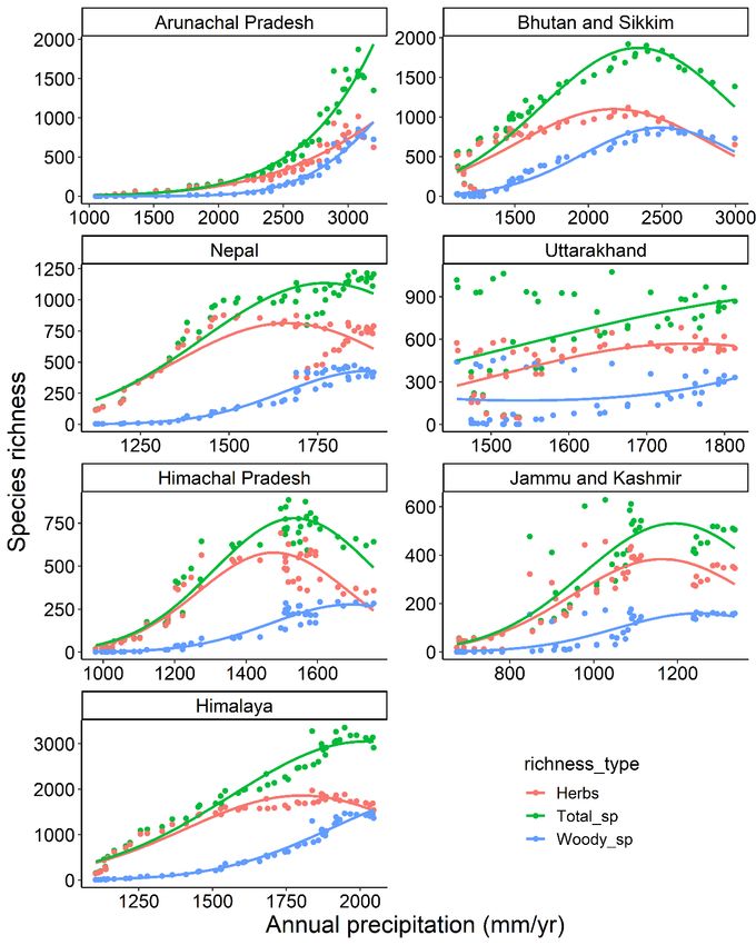
Journal
Frontiers of Biogeography
Publication year: 2021
Issue: 13.3
Article doi: doi:10.21425/F5FBG49459
Article number: e49459
Article format: Long (author names in front page + abstract + 6-10 keywords)
Article type: Research Article
Article series: Not applicable to this article
Title: A pan-Himalayan test of predictions on plant species richness based on primary production and
water-energy dynamics
Subtitle: n.a.
Author list:
Kuber P. Bhatta https://orcid.org/0000-0001-7837-1395
Benjamin A. Robson https://orcid.org/0000-0002-4987-7378
Madan K. Suwal (no orcid id)
Ole R. Vetaas https://orcid.org/0000-0002-0185-1128

Strapline author: Bhatta et al.
Strapline running title: Climatic factors controlling diversity
Supplementary Materials: Yes (1 appendix and 3 tables, 1 figure)

A pan-Himalayan test of predictions on plant species richness based
        on primary production and water-energy dynamics
Kuber P. Bhatta1*, Benjamin A. Robson2, 3, Madan K. Suwal4 and Ole R. Vetaas4

1
    Department of Biological Sciences, University of Bergen, Bergen, Norway.

2
    Department of Earth Science, University of Bergen, Bergen, Norway.

3
    Bjerknes Centre for Climate Research, Bergen, Norway.

4
    Department of Geography, University of Bergen, Bergen, Norway.

*Correspondence: Kuber P. Bhatta, Kuber.Bhatta@uib.no

    This paper is part of an Elevational Gradients and Mountain Biodiversity
    Special Issue

                                                                                                   1
Abstract

Spatial variation in plant species diversity is well-documented but an overarching first-

principles theory for diversity variation is lacking. Chemical energy expressed as Net Primary

Production (NPP) is related to a monotonic increase in species richness at a macroscale and

supports one of the leading energy-productivity hypotheses, the More individuals Hypothesis.

Alternatively, water-energy dynamics (WED) hypothesizes enhanced species richness when

water is freely available and energy supply is optimal. This theoretical model emphasises the

amount and duration of photosynthesis across the year and therefore we include the length

of the growing season and its interaction with precipitation. This seasonal-WED model

assumes that biotemperature and available water represent the photosynthetically active

period for the plants and hence, is directly related to NPP, especially in temperate and alpine

regions. This study aims to evaluate the above-mentioned theoretical models using

interpolated elevational species richness of woody and herbaceous flowering plants of the

entire Himalayan range based on data compiled from databases. Generalized linear models

(GLM) and generalized linear mixed models (GLMM) were used to analyse species richness

(elevational gamma diversity) in the six geopolitical sectors of the Himalaya. NPP, annual

precipitation, potential evapotranspiration (derived by the Holdridge formula), and length of

growing season were treated as the explanatory variables and the models were evaluated

using the Akaike Information Criterion (AIC) and explained deviance. Both precipitation plus

potential evapotranspiration (PET), and NPP explain plant species richness in the Himalaya.

The seasonal-WED model explains the species richness trends of both plant life-forms in all

sectors of the Himalayan range better than the NPP-model. Despite the linear precipitation

term failing to precisely capture the amount of water available to plants, the seasonal-WED

                                                                                             2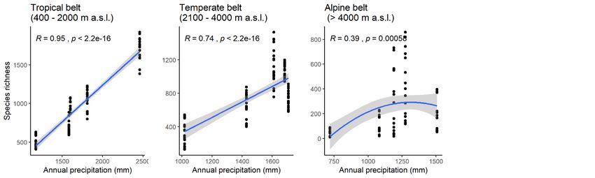
model, which is based on the thermodynamical transition between water phases, is

reasonably good and can forecast peaks in species richness under different climate and

primary production conditions.

Highlights

   •   The spatial pattern of plant species richness across the Himalaya can be explained by

       an interaction of water, energy, and their seasonal variation (length of the growing

       season LGS).

   •   We found that a Water-energy Dynamics (WED) model, which takes into account both

       kinetic thermal energy and water as drivers of plant species richness, explains spatial

       variance in plant species richness better than the Net Primary Production (NPP) model

       estimated by earth observation tool (MODIS), which only considers chemical energy.

   •   By incorporating the seasonal temporal dimension, i.e., LGS (~ photosynthetic active

       period for the plants) in the WED model, especially for the high-elevation areas, it is

       possible to improve fits of the WED models.

   •   The seasonal-WED model, which considers water and energy in both the kinetic as well

       as chemical form as the drivers of plant species richness, provides a more flexible array

       of regional species richness models, with better statistical fit, than the simple NPP

       model.

   Keywords: Elevational gradient, Gamma diversity, Growing season, Himalaya, Net

   primary production, Species richness, Water-energy dynamics.

                                                                                              3
Introduction
A well-supported hypothesis in ecology and biogeography is that increased thermal energy
promotes higher species diversity (Wright 1983, Currie 1991, Brown et al. 2004, Clarke and
Gaston 2006, Brown 2014). However, paradoxically, climate change, especially rising global
and local temperatures, is expected to cause species extinction (IPCC 2018, IPBES 2019) rather
than increasing species diversity. This paradox may, in part, be resolved by the synergetic
effect that expanding human land-use together with climate change has on species by
preventing their climate change-driven translocation, which in turn leads to species extinction.
However, it may also be that the energy alone is insufficient to explain biodiversity and ought
to be replaced by a better model focusing on water as well as energy. It is a basic biological
fact that life on the Earth evolved in water and there is no life without liquid water. It is
therefore unconvincing that many models on macroscale species diversity do not include
water but focus on how energy promotes species diversity by regulating metabolism,
population size, and speciation rate (Evans et al. 2005, Clarke and Gaston 2006). These energy-
based models may convincingly explain why there are so many species in the warm equatorial
sector and so few at the cold poles (Brown 2014), but fail to explain why the subtropics and
warm-temperate sectors, which despite being relatively energy-rich, have low productivity
levels and relatively few species (Vetaas et al. 2019). Such models also fail to explain species
diversity variation along elevation gradients, where many organismal groups have peaks at
intermediate elevations, and not in the warm tropical/subtropical lowland (Rahbek 1995). This
may relate to optimal moisture conditions at mid-elevations compared to the summits (frost)
and lowland (high evapotranspiration) (Peters et al. 2019, Vetaas et al. 2019, and references
therein).
4Globally, the spatial variation in species diversity in space is a well-documented pattern,
encompassing the decline in species richness from the equatorial tropics to the Artic and the
commonly found unimodal pattern along extensive tropical mountain ranges (Rahbek 1995,
Hawkins 2001, Steinbauer et al. 2016). Although several studies have shown a remarkably
strong association between contemporary climate and species richness (Rohde 1992, Currie
et al. 2004, Kreft and Jetz 2007, and references therein), there is still no consensus-theory on
the mechanisms that determine species richness patterns on our planet. This is in fact the
major unexplained pattern in natural history (cf. Jablonski et al. 2006). The empirical evidence
and correlations with climate across many lifeforms and taxonomic levels have, however,
generated many conjectures and hypotheses, and some constituent models and theories
(Scheiner et al. 2011), such as the equilibrium theory of biodiversity dynamics (Scheiner et al.
2011, Storch and Okie 2019) and the metabolic theory of ecology (MTE) (Brown et al. 2004).
The latter model, MTE, links environmental energy to the rate of metabolism (Brown et al.
2004), but unfortunately, it cannot be tested along thermal gradients because it assumes no
water limitation (Vetaas et al. 2019). Another group of theorising focus on energy- and
productivity often expressed as actual evapotranspiration (Currie 1991, Rohde 1992, Currie et
al. 2004). One explanation is that high energy availability increases the number of individuals
that can be supported, allowing species to maintain larger populations, which then have a
reduced extinction risk. The lowered probability of extinction thus elevates species richness in
high-energy assemblages. This is often referred to as the More Individuals Hypothesis (MiH).
MiH has a probabilistic philosophy, where NPP will generate more individuals, which, in turn,
will increase the probability of more co-occurring species and survival of small populations
(Wright 1983, Srivastava and Lawton 1998). The link between energy, individuals, and species
richness has recently been challenged by Storch et al. (2018), while Lavers and Field (2006)
5argue that this link is not needed for a mechanistic species diversity theory. One possible
reason for the lack of consensus is a focus on energy per se and too little focus on energy as a
regulator of available liquid water. Although the importance of water for biodiversity is an
established idea (cf. Hawkins et al. 2003), currently, the most detailed expression of this tenet
is biological relativity of water-energy dynamics (WED), which has been articulated by O'Brien
(1993) and O'Brien et al. (1998) and was elaborated to a preliminary constituent theoretical
model by O'Brien (2006) (Vetaas 2006). Following this rationale, Hawkins et al. (2003) and
Field et al. (2009) argue that any theoretical reasoning that overlooks water and water-energy
interactions is missing a key component for explaining broad-scale patterns of species
diversity. Liquid water as a limited resource is a crucial point because in the non-tropical areas
water will potentially be unavailable due to water being frozen for durations ranging from a
few days to almost the entire year, and the sensitivity of most plants to frost or drought may
constrain their richness outside warm and humid regions (Currie et al. 2004). This will directly
influence biological activity and hence the time available for metabolism and sexual
reproduction, and thereby affects evolutionary speed and genetic diversity. From an
evolutionary perspective, Gillman & Wright (2014) also point to water and thermal energy as
drivers of evolutionary speed, and there is evidence that hotspots of species richness and high
diversification rates may coincide, but it is not necessarily a general pattern (Steinbauer et al.
2016, Quintero and Jetz 2018).
The tenet of WED is simple: species richness will increase as thermal energy increases, but
beyond a certain threshold, water deficits due to high evapotranspiration demand will reduce
plant activity and ultimately richness, while water freezing at the cold end of the gradient also
limits plant activity (O'Brien 1998, Hawkins et al. 2003, McCain 2007). Species richness,
6particularly of plants, is thus dependent on both water and energy. The linear response to
precipitation and the unimodal response to potential evapotranspiration (PET) enable this
model to predict unique peaks for different plant life-forms, whereas models based on energy-
productivity model will predict a similar optimum for most organisms. This is because most
energy- and productivity-based models, independent of the expression of energy (thermal
energy and environmental temperature) predict linear responses in richness along a
productivity-energy gradient (Wright 1983, Evans et al. 2005, Clarke and Gaston 2006, Gillman
et al. 2015, and references therein). In contrast, WED models predict a parabolic response in
richness as a function of PET (Fig. 1). The Energy-productivity models, such as NPP, may also
predict a linear increase, but this depends on the relationship between productivity and
elevation which may be unimodal or curvilinear rather than strictly linear.
Based on this theoretical background we aim to evaluate whether the WED model or the
energy-productivity model (NPP) better explains the spatial variation in species richness. This
is done for interpolated elevational species richness based on data compiled from databases
of woody and herbaceous flowering plants across the entire Himalayan range. In addition, on
a coarse scale, we will test if there is a linear trend in richness as a function of precipitation
from the drier western Himalayas to the moist eastern Himalayas, which can be deduced from
the WED model. If WED explains the spatial variation in species richness better than NPP, it
may indicate that WED provides a better mechanistic explanation of plant species richness
than energy-productivity theories do. If NPP is superior it may indicate richness can be better
explained by arguments related to the potential chemical energy of biomass than the
dynamics of water and kinetic energy.
7Material and Methods
Location and physiography
The Himalaya (c. 97o 30´ E – 72o 30´E longitudes and c. 27o N – 29 o N (east), c. 27o N – 30 o N
(central) and c 29o N – 36o N (west) latitudes) is the highest mountain system in the world,
separating the Tibetan Plateau from the Indian subcontinent in South Asia (Fig. 2). The
Himalaya lies in the contact zone of the Indian Plate and the Eurasian Plate and extends over
a c. 2500 km southward-convex arc from east-southeast to the west-northwest (Singh and
Singh 1987). It borders with the upper streams of the Brahmaputra in the east, Indus River
and Naga Parbat in the west, the Tibetan Plateau in the north and the Indo-Gangetic Plains to
the south. From west to east, the Himalaya spans over five geopolitical sectors (Jammu and
Kashmir Himalayas, Kumaun and Garhwal Himalayas, Nepal Himalayas, Sikkim and Bhutan
Himalayas and Assam Himalayas), and has a profound effect on regulating the climate and
biodiversity of the region (Gansser 1964, Le Fort 1975). The complex physiography of this
mountain range encompasses the largest elevational gradient on Earth (from sea level to over
8000 m above sea level) and can be broadly divided into three major east-west cis-zones: the
Siwalik Range (100–1500 m a.s.l.), the Lesser Himalaya (1500–3000 m a.s.l.) and the Greater
Himalaya (3000–8000 m a.s.l.)1.
Bioclimatic zones
1. https://www.britannica.com/place/Himalayas, last accessed 28/02/2021.
8The vast physiography of the Himalaya has resulted in a remarkable variation in topography
and climate over the region. Broadly speaking there are two seasons, a dry winter period and
a wet summer period. The dry period is characterised by wind blowing from the north-west,
whereas the wet period is characterised by the Indian summer monsoon that enters from
south-east of Himalaya and gradually drifts toward the west Himalaya. The amount and
distribution of precipitation and the duration of cloud cover varies considerably in different
parts of the region, but precipitation gradually decreases from east to west, which is the most
likely a governing factor in the variation in species richness along the east-west Himalayan axis
(Fig. 3). Along a south-north elevation gradient, precipitation generally increases from the
plains to the mid-elevations and thereafter decreases linearly towards higher elevations. Most
of the precipitation is received from mid-June to mid-September and the cis-Himalayan ranges
(to the south of the Greater Himalaya) receive more precipitation than the trans-Himalayan
ranges (north of the Greater Himalaya towards the Tibetan Plateau). Similarly, atmospheric
temperatures in the Himalaya show profound variations along the elevation gradient and
follow a decreasing pattern of c. 5 oC per 1 km rise in elevation. Thus, two enormous
bioclimatic gradients lie approximately orthogonal to each other along Himalayan axes. An
overview of the phytogeography, vegetation and climate in the Himalayan region is presented
in the Appendix S1.
Data source and selected taxa
We used the data of the flowering plants of Himalaya published by Rana et al. (2019) for
estimation of species richness. The dataset consists of 8765 native angiosperm species with
their life-forms and elevational distributions from six geopolitical sectors along east-west
Himalayan axis namely, Arunachal Pradesh, Bhutan and Sikkim, Nepal, Uttarakhand, Himachal
9Pradesh and Jammu and Kashmir. Of these, Bhutan and Nepal are countries, whereas the
remaining areas are states of India. The data we used, along with relevant metadata, such as
the spatial coverage, and data collection and standardisation procedure are also published as
an open-access database (Rana and Rawat 2017).
The life-forms and the minimum and maximum elevations of the flowering plant species in
the dataset were compiled using the published records of species in the Himalaya in the 31
local and regional Floras (see Rana and Rawat 2017, Rana et al. 2019). These Floras are based
on the plants collected and/or reported from different sub-regions of the Himalaya during the
period of 1903–2014. The authors of the database have resolved the taxonomic
nomenclature, taxon rank as well as indigenous versus exotic status of each recorded species
according to The Global Biodiversity Information Facility2 and The Plant List3 databases (Rana
and Rawat 2017). All the exotic species and those with unresolved taxonomic nomenclature
were removed from the dataset, and the potential bias in the estimation of species’
elevational limits in each Himalayan sector has also been corrected (see Rana et al. 2019).
Using the elevational ranges of the species in each region, we interpolated the species
presences in each 100-m elevation band between the upper and lower elevational limit of the
species. Realising that different species of different life-forms reveal different responses to
precipitation and temperature regimes (cf. Bhatta 2018, Bhatta et al. 2018), we estimated the
total, herbaceous and woody species richness for each sector.
We extracted bioclimatic variables for each Himalayan sector from CHELSA Bioclim Version
1.2 (Karger et al. 2017). For each sector, we also estimated the total area and NPP per 100-m
2. http://www.gbif.org/, last accessed 03/6/2017.
3. http://www.theplantlist.org/, last accessed 15/04/2017.
10elevation band using the data obtained from the Moderate Resolution Imaging
Spectroradiometer (MODIS) sensor from 2000-2018 (Running et al. 2015).
Methodological framework
The response variables
In the present study, the species richness is defined as the number of species with an
overlapping elevation range, i.e., the thermal energy range, because atmospheric
temperature is collinear with the elevation gradient (1000 m elevational difference = 5.5 oC
difference). To interpolate the species’ occurrences along an elevation gradient between 400
and 5500 m a.s.l., the elevation gradient was divided into fifty-two 100-m elevation intervals
(vertical elevation bands). A species was considered as being present in every 100-m band
between its upper and lower elevation range limits within the considered elevation gradient
(400 m – 5500 m a.s.l.). The response variable – species richness – was estimated as the total
number of species found in each 100-m elevation band, which is called elevational-gamma
diversity by Lomolino (2001). The general trend in elevational gamma diversity is broadly
similar to the overall richness trends using small plots in Nepal Himalaya (Bhatta et al. 2018).
For the analyses, we considered the elevation gradient from 400 m a.s.l. to 5500 m a.s.l. in
each sector. This was done to avoid the influence of human land-use on the species richness
estimations, especially towards the low-elevation (plain regions) of the Himalaya and also to
minimise the underestimation effect of species’ range interpolations (Grytnes and Vetaas
2002).
Moreover, we divided the entire elevation gradient into three bioclimatic belts, namely,
tropical (400 m a.s.l. – 2000 m a.s.l.), temperate (over 2000 m a.s.l. – 4000 m a.s.l.) and alpine
11(over 4000 m a.s.l.) and correlated the species richness in each bioclimatic belt with the east-
west precipitation gradient. We did this to test if the variation in species richness along cis-
Himalaya corresponds to the underlying east-west precipitation gradient. However, we
excluded Arunachal Pradesh in this analysis because this sector is considered under-sampled
(Rana et al. 2019) and hence, species richness of this sector cannot be compared directly with
that of the remaining sectors.
The explanatory variables
(a) Bioclimate variables
For each sector, we extracted four bioclimatic variables at a resolution of 30 arc seconds (1
km) - Bio1 (Annual Mean Temperature), Bio5 (Maximum Temperature of Warmest Month),
Bio 6 (Minimum Temperature of Coldest Month) and Bio12 (Annual Precipitation AP) from
CHELSA Bioclim Version 1.2 (Karger et al. 2017). These variables were extracted for each 100-
m elevation band for each Himalayan sector based on the Shuttle Radar Topography Mission
(SRTM) Digital Elevation Model (DEM).
(b) Net primary production (NPP)
Remote-sensing products have been widely used to map, monitor, and model gross primary
production (GPP) and NPP dynamics at the regional and global scale (Nemani et al. 2003, Zhao
and Running 2010). The Moderate Resolution Imaging Spectro-radiometer (MODIS), an optical
instrument installed on the Terra and Aqua satellites of the NASA Earth observation system,
provides some of the most reliable, moderate spatial and high temporal resolution standard
global GPP and NPP estimates. For estimating NPP we averaged the annual MODIS NPP
12products (MOD17A3) from 2011 to 2018 together using the Google Earth Engine and
downloaded one mosaiced file for the mean NPP to be further processed in python using the
ArcPy and NumPy packages (Running et al. 2015). The mean NPP was then extracted per 100-
m elevation band based on the SRTM elevation model. The area of each elevation band was
also extracted.
(c) Potential evapotranspiration (PET)
We estimated annual PET by using a modification of the Holdridge equation (PET = mean
annual Bio-temperature, i.e., temperature > 0 oC X 58.93) (cf. Bhattarai and Vetaas 2003). It
was not possible to estimate realistic Holdridge PET values for the extremely high elevation
belts where the biotemperature (mean annual temperature) was below 0oC. According to
CHELSA bioclimate data, 0oC in temperature is encountered at elevations much lower (at c.
4000 m a.s.l.) than the elevations in Himalaya from which biotemperature starts to become <
0 oC (at c. 5000 m a.s.l.). Therefore, for a more realistic estimation of PET, we used the
maximum temperature of the warmest month in each 100-m elevation band as a proxy of the
biotemperature.
(d) Length of growing season (LGS)
The estimation of the LGS (number of days in a year above 0 oC biotemperature) based on the
monthly averaged biotemperature data of CHELSA was too coarse as it resulted in variations
in the LGS by one month (30 days) per 100-m bands along an elevation gradient, which is
unrealistic. Therefore, we used Bio 5 and Bio 6 to estimate the rate of decrease of the growing
days per 100-m increase in elevation. Here, we estimated the number of 100-m elevation
13bands (N) between the elevations from where the Bio 5 and Bio 6 start to become negative
and divided the annual number of growing days (365) by N.
The models
We analysed two main models, Net primary production (NPP: M1) and Water-energy
dynamics (WED: M2) (Fig. 1), as defined below with respect to species richness (S). O’Brien
(1998) incorporated seasonality by using length of growing season (and PETmax – PETmin) in
one of the WED models named interim general models (IGM1-model). We follow this line of
reasoning by including an interaction term between length of growing season (LGS) and
precipitation, called the seasonal-WED (M3) (cf. Vetaas et al. 2019). M3 is an attempt to
express the temporal dimension (duration of precipitation) in the WED model. This is because
precipitation in the form of liquid water may relatively be less available at high elevation due
to a shorter growing season. LGS will also reflect productivity, which will correspond to the
duration of the year the moisture will be utilised for the biological activity (Michaletz et al.
2014).
(M1) NPP: S = f(NPP): S ~ NPP
(M2) WED: S = f(AP, PET): S ~ AP + poly(PET, 2)
(M3) seasonal-WED: S = f(AP, PET, AP*LGS): S ~ AP + poly(PET, 2) + LGS*AP
The three contrasting models (M1, M2 and M3) were fitted for the herbaceous species-,
woody- and total species richness in each of the Himalayan sector and in entire Himalayan
Mountain range. All explanatory variables were estimated for each of the 100-m elevation
bands between 400 ‒ 5500 m above sea level in each sector. In the first model (M1), energy
translates into NPP and the number of individuals, i.e., potential chemical energy. In the
14second WED model (M2), kinetic energy is translated into liquid water (mm) evaporated per
o
C increase in temperature (Holdrige’s PET (cf. Bhattarai and Vetaas 2003)). Precipitation is
estimated in millimetre per year and PET is annual potential evapotranspiration expressed in
mm per year.
The strict interim general model, developed for woody plant richness following the WED
conceptual framework (O'Brien 2006), incorporates annual rainfall and minimum monthly PET
based on a formula by Thornthwaite (1957). This use of annual rainfall and minimum monthly
PET probably originates as the model was developed in South Africa, where snowfall is very
rare (and hence, rainfall = precipitation), and minimum PET was used to capture seasonality
of thermal regime. However, here we evaluate a more flexible WED model that includes not
only the woody plants in a region where snowfall is common and where the minimum mean
monthly PET will be insufficiently discriminating (Moser et al. 2005). Therefore, we use
precipitation and annual PET, as suggested by the Holdridge equation (cf. Bhattarai and Vetaas
2003). We evaluate a WED model including precipitation and annual PET, versus an NPP model
including estimated NPP with respect to elevational interpolated species richness of
angiosperms across the Himalaya. For each Himalayan sector, elevational patterns of the
explanatory variables in the M1, M2 and M3 are presented in Fig. 4.
Model assessment
We fitted all the species richness models described above using generalised linear models
(GLM) and generalised linear mixed models (GLMM) within the maximum likelihood
framework, assuming a Poisson distribution of error. We compared the performance of the
area-unaccounted as well as the area-accounted models using Akaike’s Information Criterion
15(AIC) and deviance explained in the model. The variables included are theoretically justified
from the two potential general theories of species biodiversity described above. Primarily, we
aim to compare NPP and our WED model, and the latter model is then elaborated with an
interaction term (M3, seasonal-WED). The AIC measures the relative likelihood of the model’s
performance and is proportional to the likelihood of the model and the number of parameters
used to generate it. The best model is the one with the lowest AIC (less Kullback-Leibler
information is lost), and other models are usually considered less plausible if the difference in
AIC between them is larger than two AIC values. Hence, a difference value of AIC < 2 indicates
that a model is equally good (Burnham and Anderson 2002). In addition, we used deviance
explained to evaluate the models (NPP vs. WED vs. seasonal-WED).
If the AIC indicated that a second-order energy term needs to be included, we performed a
chi-test on the precipitation term to elucidate whether it has any explanatory power in
addition to the PET terms. Precipitation is a difficult variable to model because it is a resource
gradient that an organism may consume (in contrast to energy, which is a regulator gradient)
and can move away from where it was deposited. We therefore performed a post-hoc
elaboration of our original WED model, i.e., included an interaction term of precipitation and
length of growing season (LGS) (M3).
Finally, we tested the influence of the potential co-variate area on the observed patterns. For
this, we applied three well-established approaches: First, following the procedure of Galmán
et al. (2018), we extracted the residuals of each model and performed regression against area
as a predictor variable to see if there is significant influence of area on the observed patterns
after accounting for the main explanatory factors. Secondly, for each Himalayan sector, we
added the area of each 100-m elevation band as a first term variable in the NPP, WED and
16seasonal-WED model and then compared the AIC values of the models. Thirdly, we performed
a Generalised Linear Mixed Model (GLMM) analysis for each of the contrasting species
richness models using “lme4” package in R (Bates et al. 2015). Here, we fitted four different
mixed models for each of the competing model, considering “area” and “Himalayan sector” in
different combinations as random effect variables as well as by adding “area” to the main
explanatory variables as the fixed effect variable. Then we compared the four mixed models
using Analysis of Variance (ANOVA), which summarizes the differences in fit between the
models (Bates et al. 2015). By using “car” package in R (Fox and Weisberg 2019), we detected
the collinearity among the predictor variables by estimating the Gross Variance Inflation
Factor (GVIF) of the best fitted model of the GLMM. A predictor variable with GVIF > 10 was
considered as a collinear variable. All the analyses were performed in R3.6.3 (R Core Team
2020).
Results
The interpolated richness of 7764 species of flowering plants recorded between 400 m a.s.l.
and 5500 m a.s.l. in the Himalaya was used for analysing the variation in species richness along
the precipitation gradient of cis-Himalaya and for fitting the species richness models.
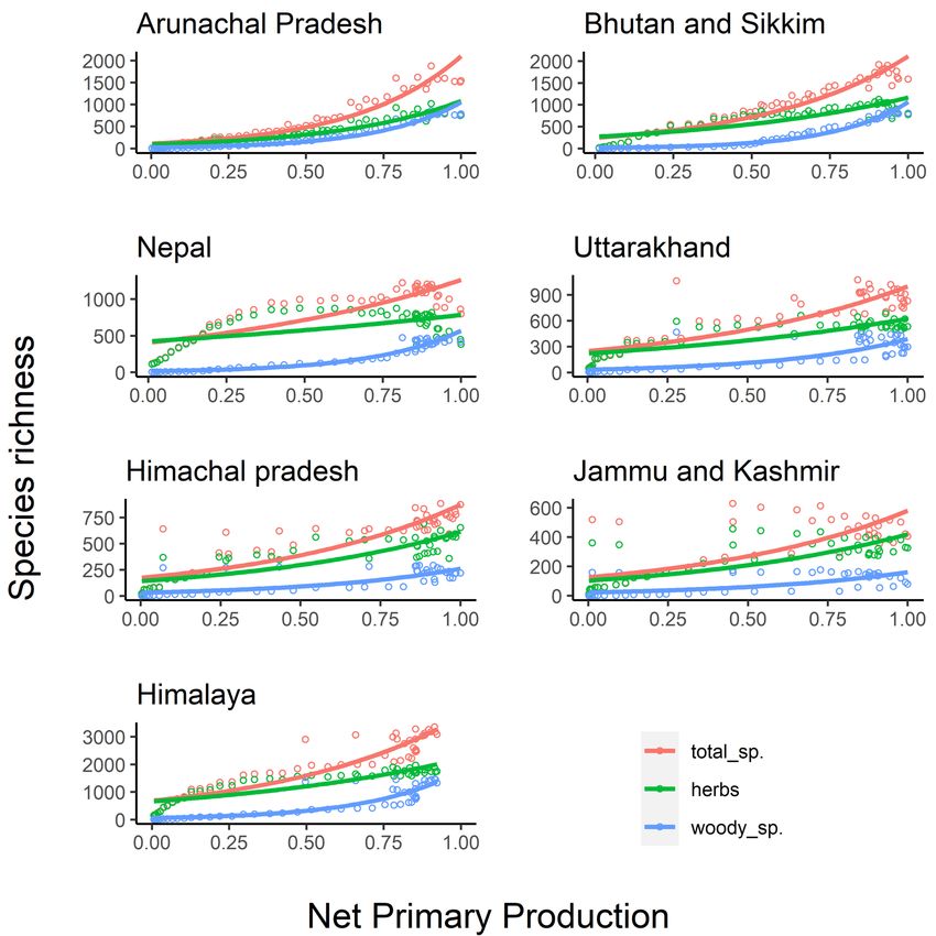
The coarse analysis across the six Himalayan sectors (Fig. 3) from the dry west towards the
moist east revealed strong responses in plant species richness as a function of precipitation in
all three elevation zones, i.e., subtropical, temperate, and the alpine zones. Variations in
species richness within the tropical and temperate zones had a linear response as predicted
by WED, whereas the same analyses for the alpine belt revealed a curvilinear response in
species richness (Fig. 3).
17The main model assessment of NPP vs WED is based on 63 GLM regression models of species
richness in the Himalayan Mountain range (9 models for each Himalayan sector as well as the
whole Himalaya, for each of which models M1, M2 and M3 was fitted for the herbaceous-,
woody- and total species richness) (Table 1, Table S1).
The net primary production model (M1) had much higher AIC values and lower percentage
deviance explained than the WED model (M2), which holds true for total-, herbaceous- as well
as woody-species richness of all Himalayan sectors and of the entire mountain range (Table
1). This indicates that the WED model captured more of the variation in species richness than
the NPP model (Table 1, Figs. 5, 6, 7). Although herbaceous and woody species richness peak
at different points along the energy-elevation gradient in the six sectors of Himalaya,
variations in richness of the two plant life-forms tend to show similar responses to the water
and energy gradients (WED model) within each sector, although also strongly contrasting
responses are noticeable between sectors (Fig. 6, 7, Table S2).
The WED models were superior to the NPP model in terms of AIC and percentage deviance
explained by the model. However, the correlation between annual precipitation term and
species richness in the WED models varied across the plant life-forms and across the
Himalayan sectors (Fig. 7). The seasonal-WED model (M3), with an interaction term between
length of growing season (LGS) and precipitation (MAP), further improved the variation
explained, particularly for herb richness (Table 1). However, the seasonal-WED models for the
woody species richness are inconsistent with respect to individual terms and their statistical
significance.
18We evaluated each model by checking how much of the residual deviance could be correlated
with area in each of the elevation-bands. Area was statistically significant in most of the NPP
models for different plant life-forms, whereas area was statistically insignificant in all WED
and seasonal-WED models (Table 2, Table S3a). However, area appeared as a statistically
significant co-variate when we included it as a first term variable in each model, and also when
treated it as a random as well as fixed effect variable in the generalised linear mixed models.
Even so, including the area of each 100 m elevation belt did not influence the relative
performance of the competing species richness models. Among the area-included models, the
seasonal-WED model always performed slightly better than the WED model and the WED
revealed significantly better-fit than the NPP model (Table S3b, S3c).
Estimations of the Generalized Variance Inflation Factor (GVIF) in the best-fitted mixed models
revealed that length of the growing season (LGS) (GVIF = 12.38) and potential
evapotranspiration at a second order polynomial (GVIF = 4.74) are highly correlated in the
seasonal-WED model. However, LGS in an interaction with precipitation has lowest GVIF value
(GVIF = 1.82) in the model (Table S3c).
Discussion
The comparison of the three species richness models based on GLM regression parameters
revealed significant differences between the models, where the seasonal-WED model explains
best the species richness patterns, followed successively by the standard WED model and the
NPP model. Although the NPP model explains a significantly high proportion of the variation
in richness (Fig. 5; Table 1), the seasonal-WED model has much lower (0.1 to 0.4 times) AIC
values than the NPP model. This illustrates that the WED model in general, and the seasonal
19version in particular; capture the variation in richness much better than NPP alone. The NPP
estimates by ‘MODIDS NPP products’ are of course also a function of energy, nutrients, and
water in the soil (Zhao and Running 2010, Running et al. 2015), which illustrates why WED
and energy-productivity models belong to the same research programme (Gillman et al.
2015). However, the models differ in addressing how energy influences species richness. The
energy-NPP model assumes the influence of net primary production, i.e., potential (chemical)
energy synthesised by the vegetation on species richness, whereas we argue that the WED
hypothesis proposes regulation of biodiversity by kinetic form of thermal energy by
influencing the availability of liquid water (and hence primary production and subsequent
biological activity) in the biological system. These results lead to the question: why do the
WED models perform much better than the Energy-productivity model expressed as NPP?
Role of energy
Both herbs and woody plant richness have peaks in the lower half of the entire spatial energy
elevation gradient in all sectors (Fig. S1). These peaks in herbaceous and woody species
richness may differ within a sector (cf. Vetaas and Grytnes 2002, Bhatta et al. 2018, Rana et
al. 2019). However, overall variations in richness of both the life-forms in response to the
thermal energy elevation gradient was approximately similar across the Himalayan sectors.
This implies thermal energy is a core regulator of plant species richness regardless of the plant
life-forms. This corroborates with the underpinning mechanism that generate the richness
patterns, i.e., all plants have an upper and lower thermal energy limit (Whittaker 1967), and
more species may potentially overlap in the middle of the extensive elevation-energy gradient
because this is far away from areas that may at a long time scale experience glaciation or
desertification (cf. McCain 2007, Sun et al. 2020).
20The second order polynomial PET-term in the WED model captures this pattern in richness
much better than NPP, although the NPP has peaks at lower to mid-elevations in several of
the Himalayan sectors, where the richness peaks (Fig. 4). There is, however, considerable
confusion related to causal links between species richness and energy-productivity (Whittaker
2010, Craven et al. 2020). Many authors point to the issue of scale; in general, the relationship
strengthens at coarser scales (Wright 1983, Currie et al. 2004, Craven et al. 2020, and
references therein). The spatial scale of this current study has a huge environmental extent
(subtropical to alpine), but the spatial resolution is coarser than the landscape scale and much
finer than the macro-scale studies with grain size of 50 x 50 km or 100 x 100 km. The scale of
this study is in a range that the single term model of NPP should have a fair chance to explain
a large proportion of the variation in plant species richness (cf. Craven et al. 2020). Although
NPP provides a fairly good model, the seasonal-WED model with four terms is much better
according to the AIC-values (0.1-0.4 times smaller AIC values). This was unexpected if one
takes into consideration that AIC is designed to penalize the models with several terms
compared to those with few or one, as the NPP model. This indicates that mechanisms related
to the WED model are plausible, and it is likely that PET and growing season are regulating the
amount of liquid soil water and hence, influencing the biological activity in the system
(Hawkins et al. 2003, O'Brien 2006, Whittaker et al. 2007, Cassemiro and Diniz-Filho 2010,
McCain and Grytnes 2010). This finding corroborates the patterns revealed by a similar study
from Nepal based on richness patterns of 12 taxa in response to energy gradient (Vetaas et al.
2019) and many other studies of different scale on species richness patterns along extensive
energy-elevation gradients across the globe (e.g., Hawkins et al. 2003, Rahbek 2005, McCain
and Grytnes 2010, and references therein, Sun et al. 2020).
21The causal link between high PET and lower richness in the warm subtropical lowlands
(O'Brien 2006), is not as clear as the aforementioned temperate to alpine parts of the thermal
gradient. Although it is probable that extreme high potential evapotranspiration limits the
amount of liquid soil-water to be used by species and consequently, resulting in low species
richness in the lowland, there is also a substantial influence of human land-use, particularly
related to forestry and agriculture within these regions (Vetaas and Grytnes 2002, Nogués-
Bravo et al. 2008). The drop in richness in warm tropical and subtropical lowland in the
foothills of large mountain ranges (Rahbek 2005, and references therein) was for instance not
reported from a multi-organism study in Kilimanjaro based on field sampling in landscapes
with low human footprints (Peters et al. 2016).
Role of water-energy interaction
In addition to parabolic response in richness as function of PET (cf. above), one may deduce a
linear response in richness as a function of precipitation, which was tested across the
Himalayan sectors as depicted in Figure 3. We found a significant correspondence between
west-east variation in species richness and the underlying precipitation gradient (Fig. 3), which
supports the proposition that precipitation is an important driver of plant species richness.
This finding corroborates partly the inferences of many regional studies (e.g., Rana et al. 2019,
Chen and Su 2020, Sun et al. 2020) and global studies on climatic drivers of species richness
(Francis and Currie 2003, Kreft and Jetz 2007). However, a closer examination of the WED-
models reveals some variation in the richness-precipitation relationship across the Himalaya,
where species richness in general starts to decline from c. 1500-2000 mm precipitation,
resulting in a curvilinear response of species richness along the precipitation gradient (Fig. 7,
Table S2). The most likely cause of this discrepancy is that the WED models' annual
22precipitation term is derived from the CHELSA bioclim Bio12, which is a composite variable
that involves not only annual rainfall but also snow, which is not necessarily used for
photosynthesis in the location where it is deposited. This, along with several other factors such
as slope inclination, sun and wind exposure, soil temperature, soil texture, wind direction and
speed, and atmospheric humidity, all affect the liquid water supply to plants in mountainous
areas. As a result, annual precipitation does not accurately represent the amount of liquid soil
water available to plants. The other potential reason for this variation is that the correlation
between the east-west precipitation gradient and species richness weakens with increasing
elevation and becomes strongly linear to curvilinear (Fig. 3) where seasonality becomes an
important factor. The high elevation areas in the mountains are dominated by the herbs, for
which seasonality is as important as annual precipitation. Therefore, we have included an
interaction of the LGS and annual precipitation in the seasonal-WED model.
The rationale of the WED model relies on the crucial role of available liquid water, which is
unevenly distributed not only in space but also in time. Hence the seasonal-WED model
included the interaction of LGS and MAP (M3), which improved the explanatory power of the
model, as indicated by lower AIC and higher explained deviance of the model as compared to
those in the M1 and M2. LGS can be used as simple and straightforward proxy for primary
production (Michaletz et al. 2014, Vetaas et al. 2019). If so, a higher explanatory power of the
seasonal-WED (M3) is absolutely reasonable because incorporating the LGS
(photosynthetically active time period ~ NPP) in the WED model means the variation explained
by M1 and M2 is integrated into a broader model (M3). However, none of the competing
energy-productivity theories has included a seasonal component, but this was done by O’Brien
(1998) for prediction of richness globally by her interim general model. Based on this line of
23reasoning, the seasonal-WED model (M3) including PET, precipitation, and its interaction with
LGS can be regarded as a unification of the NPP (M1) and WED (M2) models (Vetaas et al.
2019). Although AIC is lower and the explained deviance is higher in M3 than those in M1 and
M2, the explanatory variables (PET, MAP and LGS in different combinations) are not
statistically significant, especially for the woody species richness (Table S1). This indicates that
seasonality (such as LGS) may have a more pronounced influence on persistence and growth
of short-living (annual and biennial) herbs than on that of the perennial woody plants. A
counterargument for the inclusion of LGS in the seasonal-WED model is the correlation
between PET and LGS, which may be the case in most potential study sites. A correlation
between PET and MAP is less problematic because this is an established model (O'Brien 2006,
and references therein), and collinearity may vary from site to site, and the crucial variable is
(PET ‒ PET2) and not PET as such4. Regression models including polynomial variables in first
and second-order (as PET) and interaction term like (MAP*LGS) will inevitably cause
collinearity between the single term (e.g. LGS: VIF = 12.5) and the product (LGS*MAP = 1.8)
do not represent a statistical problem4.
The difference between the two models is also revealed concerning the covariate area, which
is a crucial factor in all species diversity studies (Whittaker et al. 2001). As a part of the model
diagnostics, we found a correlation with area and the residuals of the NPP model, whereas
the residual of the seasonal-WED model did not have a significant correlation with area.
However, if we analyse all the sectors simultaneously in a mixed model approach (GLMM)
with the area as a random factor, it is clear that area is an underpinning variable for all the
4. https://statisticalhorizons.com/multicollinearity, last accessed 10/02/2021.
24models, though least significant in WED model, and notably, it does not alter the fact that the
WED models provide superior fits to the NPP model.
Conclusions
WED and seasonal-WED models address the roles of water and energy in both kinetic (PET)
(O'Brien 2006) and potential form (LGS/productivity) (Vetaas et al. 2019), and hence, explain
better the variation in species richness in a biological system than a simple NPP model. The
latter model focuses solely on metabolic (potential) energy, and hence, fails to adequately
explain variations in species richness. The seasonal-WED model includes the key climatic
factors that represent different forms of energy and water, and therefore, allows the model
to be more flexible and with better statistical fit. However, the linear precipitation term does
not always reflect the available liquid water in these mountainous environments. This model
is almost the only theoretical framework of biodiversity that is based on the first principles of
thermodynamics where energy controls the dynamic relationship of the physical state and
availability of water (O'Brien et al. 1998, O'Brien 2006) and thus its availability in time and
space for biological life. It also captures the long-term perspective because it is always safe
from an evolutionary perspective to be far away from areas that may be overheated
(desertification) or covered by glaciers, which is implicit in the theoretical framework of WED.
However, distinguishing the role of different operational forms of energy in this model would
be vital for a proper elucidation of the mechanisms of species richness patterns. Our findings
illustrate that plant species richness is inevitably related to energy, but the causal link between
energy, productivity, and species richness is weak in this study; in contrast, energy as a
regulator of liquid water resources provides a more mechanistic explanation of species
richness based on the first principles of thermodynamics.
25Acknowledgments
KPB acknowledges funding received from European Research Council Advanced Grant (grant
agreement No 741413) project “Humans on Planet Earth - Long-term impacts on biosphere
dynamics (HOPE)”. ORV received funding from L. Meltzer’s College Fund at University of
Bergen.
Author Contributions
KPB: Conceived the ideas, analysed data, and led writing; BAR: Provided data, manuscript
editing; MKS: Provided data, manuscript editing; ORV: Conceived the ideas, contributed to
writing, manuscript editing.
Data Availability
Species richness data used in the study are available in Rana at al. (2019) and in Rana and
Rawat (2017).
Supplementary Material
The following materials are available as part of the online article at
https://escholarship.org/uc/fb
Appendix S1. An overview of the phytogeography, vegetation, and climate in the Himalayan
region.
Table S1. Summary statistics of three species diversity models based on Generalised Linear
Models (GLM) analysis of the flowering plant species richness in six geopolitical sectors along
Himalayan mountain range.
26Table S2. Generalised Linear Models (GLM) regression of the flowering plant richness in six
geopolitical sectors along the Himalayan mountain range, where species richness is the
response variable and potential evapotranspiration (PET) and annual precipitation
(precipitation) are the predictor variables.
Table S3a. Generalised Linear Model (GLM) regression with residuals of three plant species
diversity models for each Himalayan sector as the response variable and area of sector as a
predictor variable.
Table S3b. Summary statistics of the three species diversity models based on Generalised
Linear Models (GLM) regression of the flowering plant species richness in the six Himalayan
sectors, where each model is first fitted as such and then by including area per 100-m
elevation band (Area) as a first term in the model.
Table S3c. Outputs of Generalised Linear Mixed Model (GLMM) regression of the three species
diversity models, where “area” per 100-m elevation belt (area) and “Himalayan sector” (6 level
factor = sector) are the random effect variables.
Figure S1. Flowering plant species richness along elevation gradient in the six Himalayan
sectors.
References
Bates, D., Mächler, M., Bolker, B.M. & Walker, S.C. (2015). Fitting Linear Mixed-Effects
Models Using lme4. Journal of Statistical Software, 67, 1–48.
https://doi.org/10.1073/pnas.1713819115
27Bhatta, K.P. (2018). Spatiotemporal dynamics of plant assemblages under changing climate
and land-use regimes in central Nepal Himalaya. PhD thesis, pp. 78. University of Bergen,
Bergen.
Bhatta, K.P., Grytnes, J.-A. & Vetaas, O.R. (2018). Scale sensitivity of the relationship
between alpha and gamma diversity along an alpine elevation gradient in central Nepal.
Journal of Biogeography, 45, 804–814. https://doi.org/10.1111/jbi.13188
Bhattarai, K.R. & Vetaas, O.R. (2003). Variation in plant species richness of different life
forms along a subtropical elevation gradient in the Himalayas, east Nepal. Global Ecology
and Biogeography, 12, 327–340. https://doi.org/10.1046/j.1466-822X.2003.00044.x
Brown, J.H. (2014). Why are there so many species in the tropics? Journal of Biogeography,
41, 8–22. https://doi.org/10.1111/jbi.12228
Brown, J.H., Gillooly, J.F., Allen, A.P., Savage, V.M. & West, G.B. (2004). Toward a metabolic
theory of ecology. Ecology, 85, 1771–1789. https://doi.org/10.1890/03-9000
Burnham, K.P. & Anderson, D.R. (2002). Model selection and multimodel inference: a practical
information-theoretic approach. Springer, New York.
Cassemiro, F.A.S. & Diniz-Filho, J.A.F. (2010). Deviations from predictions of the metabolic
theory of ecology can be explained by violations of assumptions. Ecology, 91, 3729–3738.
https://doi.org/10.1890/09-1434.1
28Chen, W.-Y. & Su, T. (2020). Asian monsoon shaped the pattern of woody dicotyledon
richness in humid regions of China. Plant Diversity, 42, 148–154.
https://doi.org/10.1016/j.pld.2020.03.003
Clarke, A. & Gaston, K.J. (2006). Climate, energy and diversity. Proceedings of the Royal
Society B: Biological Sciences, 273, 2257–2266. https://doi.org/10.1098/rspb.2006.3545
Craven, D., van der Sande, M.T., Meyer, C., et al. (2020). A cross-scale assessment of
productivity–diversity relationships. Global Ecology and Biogeography, 29, 1940–1955.
https://doi.org/10.1111/geb.13165
Currie, D.J. (1991). Energy and Large-Scale Patterns of Animal- and Plant-Species Richness. The
American Naturalist, 137, 27–49. https://doi.org/10.1086/285144
Currie, D.J., Mittelbach, G.G., Cornell, H.V., et al. (2004). Predictions and tests of climate-
based hypotheses of broad-scale variation in taxonomic richness. Ecology Letters, 7, 1121–
1134. https://doi.org/10.1111/j.1461-0248.2004.00671.x
Evans, K.L., Warren, P.H. & Gaston, K.J. (2005). Species-energy relationships at the
macroecological scale: a review of the mechanisms. Biological Reviews, 80, 1–25.
https://doi.org/10.1017/S1464793104006517
29Field, R., Hawkins, B.A., Cornell, H.V., et al. (2009). Spatial species-richness gradients across
scales: a meta-analysis. Journal of Biogeography, 36, 132–147.
https://doi.org/10.1111/j.1365-2699.2008.01963.x
Fox, J. & Weisberg, S. (2019). An R Companion to Applied Regression. Sage, Thousand Oaks
CA.
Francis, A.P. & Currie, D.J. (2003). A globally consistent richness-climate relationship for
angiosperms. The American Naturalist, 161, 523–536. https://doi.org/10.1086/368223
Galmán, A., Abdala-Roberts, L., Zhang, S., Berny-Mier y Teran, J.C., Rasmann, S. & Moreira, X.
(2018). A global analysis of elevational gradients in leaf herbivory and its underlying drivers:
Effects of plant growth form, leaf habit and climatic correlates. Journal of Ecology, 106, 413–
421. https://doi.org/10.1111/1365-2745.12866
Gansser, A. (1964). Geology of the Himalayas. Interscience Publishers, London.
Gillman, L.N. & Wright, S.D. (2014). Species richness and evolutionary speed: the influence of
temperature, water and area. Journal of Biogeography, 41, 39–51.
https://doi.org/10.1111/jbi.12173
Gillman, L.N., Wright, S.D., Cusens, J., McBride, P.D., Malhi, Y. & Whittaker, R.J. (2015).
Latitude, productivity and species richness. Global Ecology and Biogeography, 24, 107–117.
https://doi.org/10.1111/geb.12245
30Grytnes, J.-A. & Vetaas, O.R. (2002). Species richness and altitude: a comparison between
null models and interpolated plant species richness along the Himalayan altitudinal gradient,
Nepal. The American Naturalist, 159, 294–304. https://doi.org/10.1086/338542
Hawkins, B.A. (2001). Ecology's oldest pattern? Trends in Ecology & Evolution, 16, 470.
https://doi.org/10.1016/S0169-5347(01)02197-8
Hawkins, B.A., Field, R., Cornell, H.V., et al. (2003). Energy, water, and broad-scale geographic
patterns of species richness. Ecology, 84, 3105–3117. https://doi.org/10.1890/03-8006
IPBES (2019). Global assessment report on biodiversity and ecosystem services of the
Intergovernmental Science-Policy Platform on Biodiversity and Ecosystem Services (ed. by E.S.
Brondizio, J. Settele, S. Díaz and H.T. Ng), pp. 1500. IPBES secretariat, Bonn, Germany.
IPCC (2018). Global Warming of 1.5°C: An IPCC Special Report on the impacts of global
warming of 1.5°C above pre-industrial levels and related global greenhouse gas emission
pathways, in the context of strengthening the global response to the threat of climate change,
sustainable development, and efforts to eradicate poverty (ed. by V. Masson-Delmotte, P.
Zhai, H.-O. Pörtner, et al.), pp. 616. Cambridge University Press, Cambridge and New York.
Jablonski, D., Roy, K. & Valentine, J.W. (2006). Out of the Tropics: Evolutionary Dynamics of
the Latitudinal Diversity Gradient. Science, 314, 102–106.
https://doi.org/10.1126/science.1130880
31Karger, D.N., Conrad, O., Böhner, J., Kawohl, T., Kreft, H., Soria-Auza, R.W., Zimmermann,
N.E., Linder, H.P. & Kessler, M. (2017). Climatologies at high resolution for the earth’s land
surface areas. Scientific Data, 4, 170122. https://doi.org/10.1038/sdata.2017.122
Kreft, H. & Jetz, W. (2007). Global patterns and determinants of vascular plant diversity.
Proceedings of the National Academy of Sciences, 104, 5925–5930.
https://doi.org/10.1073/pnas.0608361104
Lavers, C. & Field, R. (2006). A resource-based conceptual model of plant diversity that
reassesses causality in the productivity–diversity relationship. Global Ecology and
Biogeography, 15, 213–224. https://doi.org/10.1111/j.1466-8238.2006.00229.x
Le Fort, P. (1975). Himalayas: The collided range. Present knowledge of the continental arc.
American Journal of Science, 275A, 1–44.
Lomolino, M.V. (2001). Elevation gradients of species-density: historical and prospective
views. Global Ecology and Biogeography, 10, 3–13. https://doi.org/10.1046/j.1466-
822x.2001.00229.x
McCain, C.M. (2007). Could temperature and water availability drive elevational species
richness patterns? A global case study for bats. Global Ecology and Biogeography, 16, 1–13.
https://doi.org/10.1111/j.1466-8238.2006.00263.x
32You can also read