Sensitivity of Northern Hemisphere climate to ice-ocean interface heat flux parameterizations - GMD
←
→
Page content transcription
If your browser does not render page correctly, please read the page content below
Geosci. Model Dev., 14, 4891–4908, 2021
https://doi.org/10.5194/gmd-14-4891-2021
© Author(s) 2021. This work is distributed under
the Creative Commons Attribution 4.0 License.

Sensitivity of Northern Hemisphere climate to ice–ocean interface
heat flux parameterizations
Xiaoxu Shi1 , Dirk Notz2,3 , Jiping Liu4 , Hu Yang1 , and Gerrit Lohmann1
1 AlfredWegener Institute, Helmholtz Centre for Polar and Marine Research, Bremerhaven, Germany
2 Institute
          for Oceanography, Center for Earth System Research and Sustainability (CEN),
Universität Hamburg, Hamburg, Germany
3 Department Ocean in the Earth System Max Planck Institute for Meteorology, Hamburg, Germany
4 Department of Atmospheric and Environmental Sciences, University at Albany, New York, USA

Correspondence: Xiaoxu Shi (xshi@awi.de)

Received: 26 August 2020 – Discussion started: 9 November 2020
Revised: 17 May 2021 – Accepted: 25 June 2021 – Published: 5 August 2021

Abstract. We investigate the impact of three different pa-         the most realistic parameterization (3) leads to an enhanced
rameterizations of ice–ocean heat exchange on modeled sea          Atlantic meridional overturning circulation (AMOC), a more
ice thickness, sea ice concentration, and water masses. These      positive North Atlantic Oscillation (NAO) mode and a weak-
three parameterizations are (1) an ice bath assumption with        ened Aleutian Low.
the ocean temperature fixed at the freezing temperature; (2) a
two-equation turbulent heat flux parameterization with ice–
ocean heat exchange depending linearly on the temperature
difference between the underlying ocean and the ice–ocean          1   Introduction
interface, whose temperature is kept at the freezing point of
the seawater; and (3) a three-equation turbulent heat flux ap-     The growth and decay of sea ice at the ice–ocean interface
proach in which the ice–ocean heat flux depends on the tem-        are determined by the local imbalance between the conduc-
perature difference between the underlying ocean and the           tive heat flux within the ice and the oceanic heat flux from
ice–ocean interface, whose temperature is calculated based         below the ice. Because the temperature at the ice–ocean in-
on the local salinity set by the ice ablation rate. Based on       terface is determined by phase equilibrium, any imbalance
model simulations with the stand-alone sea ice model CICE,         between the two fluxes is not compensated for by changes in
the ice–ocean model MPIOM, and the climate model COS-              the local temperature, as is the case at the ice surface, but in-
MOS, we find that compared to the most complex param-              stead by ice growth or ablation. This makes the evolution of
eterization (3), the approaches (1) and (2) result in thinner      sea ice thickness very sensitive to small changes in oceanic
Arctic sea ice, cooler water beneath high-concentration ice        heat flux (e.g., Maykut and Untersteiner, 1971). Thus a re-
and warmer water towards the ice edge, and a lower salinity        alistic parameterization of flux exchanges at the ice–ocean
in the Arctic Ocean mixed layer. In particular, parameteri-        interface is important for simulating sea ice and its climate
zation (1) results in the smallest sea ice thickness among the     feedback.
three parameterizations, as in this parameterization all poten-       For the simplest parameterization, the ice–ocean system
tial heat in the underlying ocean is used for the melting of the   is simply treated as an ice bath (see Schmidt et al., 2004):
sea ice above. For the same reason, the upper ocean layer of       The temperature of the uppermost ocean grid cells is fixed
the central Arctic is cooler when using parameterization (1)       at the freezing point temperature, and any excess energy that
compared to (2) and (3). Finally, in the fully coupled climate     enters these grid cells via advection, convection, or heat ex-
model COSMOS, parameterizations (1) and (2) result in a            change with the atmosphere is instantaneously applied to the
fairly similar oceanic or atmospheric circulation. In contrast,    ice through lateral and bottom melting. Such parameteriza-
                                                                   tion is consistent with turbulence models that treat the flux

Published by Copernicus Publications on behalf of the European Geosciences Union.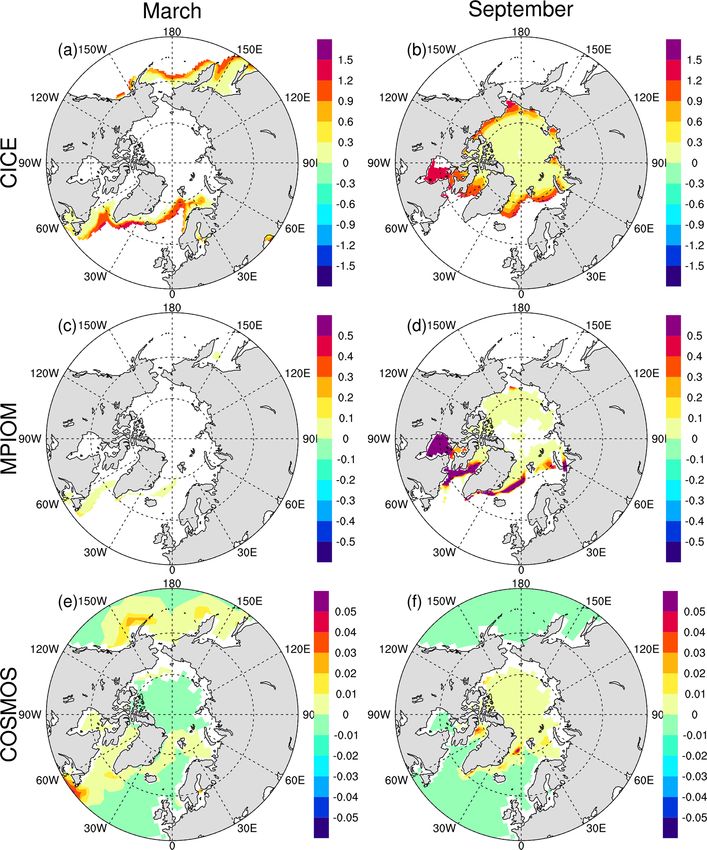
4892                                                                                            X. Shi et al.: Ice–ocean heat flux

of heat and salt as analogous to momentum flux (Josberger,          than the underlying seawater, which allows for heat fluxes
1983; Mellor et al., 1986), which results in very efficient         from the interface into the underlying ocean. This becomes
transfer whenever the ice is in motion relative to the under-       particularly important when large amounts of meltwater ac-
lying water. However, the ice bath paradigm is incompatible         cumulate underneath sea ice during summer (Notz et al.,
with observations, i.e., the 1984 Marginal Ice Zone Experi-         2003; Tsamados et al., 2015). For such more advanced for-
ment (MIZEX), which clearly indicates that an ice-covered           mulations, measurements show proportionality between heat
mixed layer can store significant amounts of heat (i.e., re-        flux and temperature difference times friction velocity across
main above freezing) for extended periods of time (McPhee,          a large range of Reynolds numbers (e.g., Fig. 6.5 in McPhee,
1986; McPhee et al., 1987; Perovich and Maykut, 1990).              2008). These formulations form the basis of many modern
These measurements demonstrate that, particularly during            sea ice models (e.g., Hunke and Lipscomb, 2010).
melting, the exchange of scalar quantities such as heat and             Exploring the behavior of different parameterizations de-
salt differs significantly from the exchange of momentum.           scribing ice–ocean heat flux has been an important topic in
The reason for this lies in the fact that, unlike ice–ocean mo-     model studies. Significant differences can generally exist be-
mentum flux, heat and mass transfer are strongly affected by        tween melt rates calculated with the three-equation approach
a thin sublayer controlled by molecular processes (McPhee           and less realistic approaches (see Notz et al., 2003; Tsama-
et al., 1987). Consistent with laboratory studies of heat trans-    dos et al., 2015), as only the three-equation approach allows
fer over hydraulically rough surfaces (Yaglom and Kader,            for heat fluxes that are directed from the interface into the
1974), the heat exchange is hence not only determined by            water and therefore allows for a realistic limitation of melt
turbulent processes but also by diffusion through this molec-       rates through the formation of a fresh water layer underneath
ular sublayer.                                                      the ice. A previous study examined the sensitivity of sea ice
   The fact that the oceanic temperature can be significantly       simulation to the approaches introduced in McPhee (1992)
higher than the freezing temperature even underneath a dense        and Notz et al. (2003) using the stand-alone sea ice model
ice cover cannot be represented in numerical models that em-        CICE (Tsamados et al., 2015). CICE uses a simple thermo-
ploy an ice bath assumption. More advanced formulations             dynamic slab ocean with fixed mixed-layer depth and seawa-
of ice–ocean heat exchange are therefore based on bulk for-         ter salinity. Thus, the realistic effect of oceanic processes can
mula, where the ice–ocean heat exchange depends linearly            not be represented. For example, the sea ice over the South-
on the temperature difference between the mixed layer and           ern Ocean is severely overestimated by CICE due to a lack
the ice–ocean interface. Early models used a constant diffu-        of warming effect from the Antarctic deep water. Therefore,
sion term as the proportionality constant (Røed, 1984), while       it is necessary to also investigate the ice–ocean heat flux for-
more advanced formulations made the heat exchange depend            mulations in a more complex system, including an interac-
on friction velocity as well (McPhee, 1992). For such more          tive ocean or even the atmosphere. Based on this motivation,
advanced formulations, measurements show proportionality            in the present study we examine how different physical re-
between heat flux and temperature difference times friction         alism, represented by the three discussed parameterizations,
velocity across a large range of Reynolds numbers (e.g.,            impacts the resulting ice cover, large-scale oceanic circula-
Fig. 6.5 in McPhee, 2008). These formulations form the basis        tion, and atmosphere properties in different numerical mod-
of many modern sea ice models (e.g., Hunke and Lipscomb,            els including an idealized columnar model, a stand-alone sea
2010).                                                              ice model, an ice–ocean coupled model, and a complex cli-
   These formulations, despite being physically much more           mate system model.
realistic than the crude ice bath assumption, often suffer from         Another motivation of our study is to help improve the
the fact that the temperature at the ice–ocean interface is sim-    formulation describing ice–ocean heat flux in various mod-
ply set as the freezing temperature of the underlying seawa-        els. For example, in the fourth version of CICE, only ice bath
ter. In reality, however, the interfacial temperature is deter-     and two-equation assumptions could be applied. In MPIOM
mined by a local phase equilibrium, and the local salinity at       and COSMOS, the ice bath approach is used, which can lead
the interface can be significantly lower than the salinity of the   to an overestimation of oceanic heat flux into sea ice. In our
seawater underneath, particularly during periods of high ab-        study, we implemented the more realistic three-equation pa-
lation rates. The interfacial temperature can be significantly      rameterization into all the models mentioned above.
higher than the freezing temperature of the underlying sea-             The paper is organized as follows. Section 2 describes
water. Therefore, one extension of the turbulent parameteri-        the parameterizations in details. Section 3 introduces vari-
zations of ice–ocean heat exchange lies in the explicit calcu-      ous models that we use for our purposes. (1) A conceptual
lation of the temperature at the ice–ocean interface based on       one-dimensional model allows us to examine a wide param-
local salinity (Jenkins et al., 2001; Notz et al., 2003; Schmidt    eter range. (2) The Los Alamos Sea Ice Model (CICE) al-
et al., 2004). Such formulations then allow for the explicit        lows us to determine changes of sea ice in a modern sea ice
calculation of heat and salt fluxes and give a more realis-         model. (3) The Max Planck Institute Global Ocean/Sea Ice
tic estimate of ice–ocean heat exchange. In particular, these       Model (MPIOM) can be used for examining the impact of the
formulations allow for the ice–ocean interface to be warmer         parameterizations on large-scale ocean circulation. (4) The

Geosci. Model Dev., 14, 4891–4908, 2021                                              https://doi.org/10.5194/gmd-14-4891-2021
X. Shi et al.: Ice–ocean heat flux                                                                                              4893

fully coupled climate model COSMOS can further help us to            be differentiated between a one-equation approach, a two-
look at the atmospheric response to the described parameter-         equation approach, and (most realistically) a three-equation
izations. Section 4 gives an overview of our experiment con-         approach. In the one-equation approach, Tinterface is simply
figuration. Section 5 describes results from sensitivity stud-       set to a constant value. We will not consider this approach
ies using the various models. We discuss and summarize our           any further here. In the more realistic two-equation approach,
main findings in Sect. 6.                                            Tinterface is set to the freezing temperature of the seawater in
                                                                     the upper-most ocean grid cell. Hence, in addition to Eq. (3),
                                                                     the freezing-point seawater is also required, which is the sec-
2   Heat flux parameterizations                                      ond equation of the two-equation approach:
The growth and decay rate ḣ of sea ice at the ice–ocean in-         Tinterface = −0.054 · Sinterface .                           (4)
terface is determined by the imbalance of the conductive heat
flux into the ice and the oceanic heat flux Foce from under-         In this (most realistic) three-equation approach, Tinterface is
neath the ice. Hence,                                                set to the freezing temperature of the water that exists di-
                 ∂T                                                  rectly at the interface. The salinity of this water is explicitly
ρi Lḣ(t) = ki      |ice + Foce ,                             (1)    calculated from a salinity balance equation:
                 ∂z
where ρi is the density of the ice, L is the latent heat of fu-      (Sinterface − Sice )ḣ(t) = αs u∗ (Smix − Sinterface ).      (5)
sion, ki is thermal conductivity of the ice, T is temperature,
and z is the vertical coordinate. Some simple sea ice models         Here, Sinterface is the salinity directly at the interface, which
assume that sea ice has no heat capacity and does not ab-            decreases during melting through the addition of fresher
sorb solar radiation. In these so-called zero-layer models, the      meltwater of sea ice with salinity Sice . Salt is exchanged with
temperature gradient is constant and simply given as the tem-        the underlying water (with salinity Smix ) through turbulent
perature difference between the ice surface and the ice bot-         exchange, with a salt exchange coefficient αS . Thus Eqs. (1),
tom, divided by ice thickness (Semtner Jr., 1976). In more           (3) and (5) form the three equations of the three-equation ap-
advanced sea ice models, the ice consists of several layers          proach. These three equations can be solved to calculate the
and the conductive heat flux into the lower most grid cell is        three unknowns ḣ, Sinterface and Tinterface .
explicitly calculated.                                                  As mentioned before, only the three-equation approach al-
   As discussed in Sect. 1, a number of approaches exist for         lows for heat fluxes that are directed from the interface into
the calculation of the oceanic heat flux Foce (see Holland and       the water. In addition, only the three-equation approach al-
Jenkins, 1999; Jenkins et al., 2001; Notz et al., 2003; Schmidt      lows for a realistic limitation of melt rates through the for-
et al., 2004). For the simplest parameterization, the ice–ocean      mation of a fresh water layer underneath the ice. For these
system is simply treated as an ice bath: the temperature of          reasons, significant differences can generally exist between
the uppermost ocean grid cells is fixed at its freezing temper-      melt rates calculated with the three-equation approach and
ature, and any excess energy that enters these grid cells via        less realistic approaches (see Notz et al., 2003).
advection, convection, or heat exchange with the atmosphere             Quantitatively, a value of 0.005 < αh < 0.006 has been
is instantaneously applied to the ice through lateral and bot-       found to give good agreement between measured and cal-
tom melting. Hence, the oceanic heat flux is given as                culated heat fluxes for a large spread of Rayleigh numbers
                                                                     (McPhee, 2008; McPhee et al., 2008). More uncertainty ex-
        ρw cw (Tmix − Tf )hmix
Foce =                         ,                               (2)   ists regarding the most appropriate values for the turbulent
                  δt                                                 exchange coefficients αh and αs for the three-equation ap-
where Tmix is ocean temperature, Tf is the salinity-dependent        proach. Their ratio R = αh /αs depends on the molecular dif-
freezing temperature, ρw is the density of the seawater, and         fusivities for heat and salt, as well as on the roughness of
cw the specific heat capacity, all determined for the upper-         the boundary (McPhee et al., 1987; McPhee, 2008). Labora-
most oceanic grid cell with vertical extent hmix ; δt is the time    tory experiments imply 35 ≤ R ≤ 70 (Owen and Thomson,
step.                                                                1963; Yaglom and Kader, 1974; Notz et al., 2003). Sire-
   In more realistic formulations, the heat flux is determined       vaag (2009) found R ≈ 33 from an analysis of field data,
from a bulk equation based on friction velocity and temper-          while McPhee et al. (2008) suggest a value of R ≈ 35. Dur-
ature difference between the mixed layer and the ice–ocean           ing freezing conditions, salt and heat are transported almost
interface according to                                               equally efficiently (McPhee et al., 2008). This is because,
                                                                     during freezing conditions, the water column is statically un-
Foce = −ρw cw αh u∗ (Tmix − Tinterface ),                     (3)
                                                                     stable owing to the salt release from growing sea ice. Hence,
where u∗ is friction velocity and αh is a turbulent heat ex-         during freezing conditions R ≈ 1 (McPhee et al., 2008), and
change coefficient (McPhee et al., 2008). A number of dif-           the two-equation approach can be used without much loss in
ferent formulations exist for the calculation of the interfa-        accuracy. The best agreement with observational data is then
cial temperature. Following Schmidt et al. (2004), these can         found for αh = 0.0057.

https://doi.org/10.5194/gmd-14-4891-2021                                                 Geosci. Model Dev., 14, 4891–4908, 2021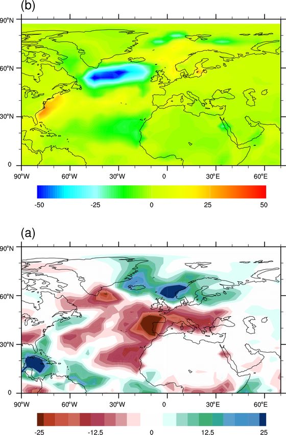
4894                                                                                        X. Shi et al.: Ice–ocean heat flux

   In testing the impact of the various parameterizations on     melt ice at the surface. We assume the sea ice in our ideal-
modeled sea ice and ocean circulation, we therefore take the     ized model to be very fresh, using a freezing temperature of
following approach: for the ice bath parameterization, we        0 ◦ C. At the ice bottom, the model calculates the change in
simply incorporate Eq. (2). For the two-equation approach,       ice thickness by balancing the conductive heat flux and the
we use Eq. (3) with αh = 0.006 and the freezing-point re-        oceanic heat flux according to Eq. (1).
lationship for seawater. For the three-equation approach, we        The seasonal variation of the atmospheric fluxes Fsw and
differentiate between freezing and melting conditions. Dur-      Fother are prescribed according to the fits provided by Notz
ing melting, we use the full three-equation approach with        (2005), approximating the monthly mean observational data
R = 35 as our reference. In an idealized 1-D model used          compiled by Maykut and Untersteiner (1971). These fits are
in our study, R = 70 is also applied to test the sensitivity
with respect to this parameter. For a certain value of R, we                      d − C1 2
                                                                 Fsw = A1 exp[B(         ) ],                                (7)
calculate αh to satisfy the requirement described in McPhee                         D1
et al. (1999). R = 35 is associated with a turbulent heat ex-                       d − C2 2
                                                                 Fother = A2 exp[B(        ) ] + E,                          (8)
change coefficient of αh = 0.0095, and R = 70 is associated                           D2
with αh = 0.0135. During freezing, we fall back to the two-
equation approach.                                               where A1 = 314, A2 = 117.8, B = −0.5, C1 = 164.1, C2 =
                                                                 206, D1 = 47.9, D2 = 53.1, E = 179.1, and d is the num-
                                                                 ber of the day in the year. The seasonal variation in surface
3     Models                                                     albedo is calculated as

We will now briefly introduce the four different models that               F
                                                                 α=                  + I,                                    (9)
we use to analyze the different response to oceanic heat flux          1 + ( d−G
                                                                              H )
                                                                                 2
parameterizations based on the ice bath assumption, the two-
equation approach, and the three-equation approach. We start     where F , G, H , and I have the values of −0.431, 207, 44.5,
with a description of our idealized columnar model with sim-     and 0.914, respectively. This equation is a fit to measure-
ple sea ice thermodynamics, then move to the stand-alone sea     ments obtained during the Surface Heat Budget of the Arctic
ice model CICE, and finally describe the ice–ocean model         Ocean (SHEBA) campaign (Perovich et al., 1999).
MPIOM and the fully coupled ice–ocean–atmosphere model              The model is coupled to an idealized oceanic mixed layer
COSMOS.                                                          of depth hmix , which can store and release heat. The cou-
                                                                 pling between the mixed-layer ocean and the sea ice via the
3.1    Idealized 1-D model                                       oceanic heat flux Foce is given by the three parameterizations
                                                                 as described above.
We use a one-dimensional columnar sea ice model coupled
to a simple ocean mixed layer to carry out sensitivity studies   3.2   CICE
and to investigate the impact of the three formulations for
ice–ocean heat exchange in an idealized setup.                   To investigate the sensitivity of sea ice to the three ice–ocean
   The model consists of a simple zero-layer sea ice model,      heat flux parameterizations in a modern sea ice model, we
where the surface temperature Ts is determined by balancing      use version 4.0 of the stand-alone sea ice model CICE. The
atmospheric fluxes and the conductive heat flux through the      model consists of a multi-layer energy-conserving thermody-
ice according to                                                 namic sub-model (Bitz and Lipscomb, 1999) with a sub-grid-
                                                                 scale ice thickness distribution and a submodel of ice dynam-
                                       Ts − Tbot
−(1 − α)Fsw − Fother + σ Ts 4 = −ki             .         (6)   ics based on an elastic–viscous–plastic rheology (Hunke and
                                           h                     Dukowicz, 1997; Hunke, 2001) that uses incremental remap-
Here, α is the albedo of the ice surface; Fsw is the shortwave   ping for ice advection (Lipscomb and Hunke, 2004). A de-
flux;  = 0.95 is the infrared emissivity; σ = 5.67 × 10⁻⁸ is    tailed model description is given in Hunke and Lipscomb
the Stefan–Boltzmann constant; Tbot is the temperature at the    (2010).
ice–ocean interface; and Fother is the sum of sensible heat         The surface temperature of the ice is calculated by bal-
flux, latent heat flux, and downward longwave radiation flux.    ancing incoming fluxes from the atmosphere with outgoing
(1 − α)Fsw + Fother represents the heat input to the surface     longwave fluxes and the conductive heat flux in the ice. For
of the ice, and σ Ts 4 represents the upward longwave radia-    the albedo, here we use the standard setup of The Community
tion flux from the ice surface. For simplicity, we assume that   Climate System Model version 3 (CCSM3), where the (spec-
the thermal conductivity of sea ice ki is constant and set to    tral) albedo is calculated explicitly based on snow and ice
ki = 2.03 W m−1 K−1 according to the 1-D thermodynamic           temperature and thickness (see Hunke and Lipscomb, 2010
sea ice model of Maykut and Untersteiner (1971). During          for details). A bulk sea ice salinity of 4 psu is implemented.
melting periods, the surface temperature is fixed at the bulk       We run CICE in stand-alone mode, coupled to the mixed-
freezing temperature of the ice and the excess heat is used to   layer ocean that forms part of the CICE package. The heat

Geosci. Model Dev., 14, 4891–4908, 2021                                          https://doi.org/10.5194/gmd-14-4891-2021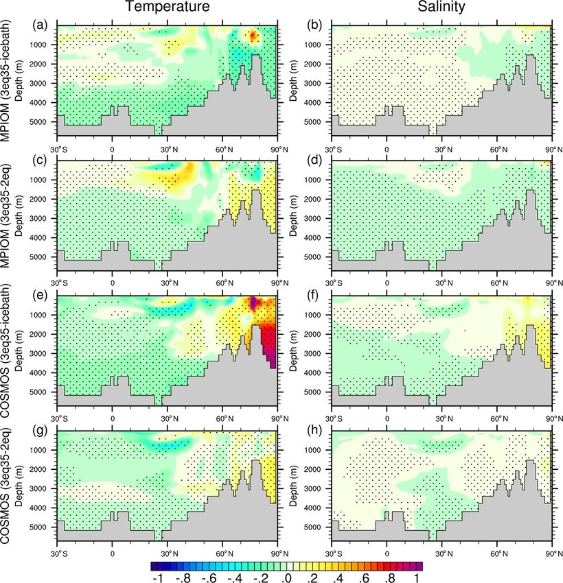
X. Shi et al.: Ice–ocean heat flux                                                                                            4895

flux between this mixed-layer ocean and the sea ice is in the       mosphere on a sphere (Roeckner et al., 2003). It is formu-
standard form of CICE described by the two-equation ap-             lated on a Gaussian grid for the horizontal transport schemes
proach with αh = 0.006. This formulation is here either used        and on a hybrid sigma-pressure grid for the vertical coor-
directly or replaced by the ice bath formulation or the three-      dinate. The OASIS3 coupler (Valcke, 2013) is used for the
equation formulation as described before. The salinity of the       coupling between the ocean and the atmosphere components.
mixed-layer in SIM and CICE is kept at 34 g kg−1 .                  Once per simulated day, solar and non-solar heat fluxes, hy-
                                                                    drological variables, and horizontal wind stress are provided
3.3   MPIOM                                                         from the atmosphere to the ocean through OASIS3. At the
                                                                    same time, the ocean provides its sea ice coverage and the
To examine the interaction of changes in the sea ice model          sea-surface temperature to the atmosphere.
with large-scale ocean circulation, we use the ocean gen-
eral circulation model MPIOM (Max Planck Institute Ocean
Model). MPIOM is based on the primitive equations with              4   Experimental design
representation of thermodynamic processes (Marsland et al.,
                                                                    For each model, we perform separate simulations based on
2003). The orthogonal curvilinear grid is applied in MPIOM
                                                                    the three ice–ocean heat flux formulations (see Table 1). We
with the north pole located over Greenland. The relevant
                                                                    assume that the three-equation approach with R = 35 de-
terms of the surface heat balance are parameterized accord-
                                                                    scribes reality more realistically and hence use this simula-
ing to bulk formulae for turbulent fluxes (Oberhuber, 1993)
                                                                    tion as our reference. In our idealized 1-D model, we also use
and radiant fluxes (Berliand, 1952).
                                                                    R = 70 to test the model sensitivity with respect to this pa-
   The sea ice component of MPIOM uses zero-layer thermo-
                                                                    rameter. For a given value of R, we calculate αh to satisfy the
dynamics following Semtner Jr. (1976) and viscous–plastic
                                                                    requirement described in McPhee et al. (1999). This results
dynamics following Hibler III (1979). It does not allow for
                                                                    in a turbulent heat exchange coefficient αh = 0.0095 for R =
a sub-grid ice thickness distribution. The sea ice state within
                                                                    35 and αh = 0.0135 for R = 70. In SIM and CICE the mixed-
a certain grid cell is hence fully described by ice concentra-
                                                                    layer salinity has a constant value of 34 g kg−1 . In MPIOM
tion C and ice thickness h. The surface heat balance is solved
                                                                    and COSMOS the salinity of the seawater evolves dynami-
separately for the ice-covered and ice-free part of every grid
                                                                    cally in response to oceanic or atmospheric processes.
cell. Any ice that is formed through heat loss from the ice-
                                                                       As atmospheric forcing, we use Eqs. (7) to (9) for our con-
free part is merged with the existing ice to form a new ice
                                                                    ceptual 1-D model. For CICE, we use the National Center for
thickness and ice concentration. The change in sea ice thick-
                                                                    Atmospheric Research (NCAR) monthly mean climatologi-
ness and concentration can be calculated via two main ice
                                                                    cal data with 1◦ × 1◦ resolution Kalnay et al. (1996). Input
distribution parameters as outlined by Notz et al. (2013), the
                                                                    fields contain monthly climatological sea surface tempera-
first one being a so-called lead closing parameter that de-
                                                                    ture, sea surface salinity, the depth of ocean mixed layer, sur-
scribes how quickly the sea ice concentration increases dur-
                                                                    face wind speeds, 10 m air temperature, humidity, and radi-
ing new ice formation processes, and the other describing
                                                                    ation for the time period 1984–2007. For MPIOM, we use a
the change in the ice thickness distribution during melting.
                                                                    GR30 (about 3◦ ) horizontal resolution and 40 uneven verti-
In its standard setup, MPIOM uses an ice bath parameteriza-
                                                                    cal layers, forced by daily heat, freshwater, and momentum
tion to calculate the heat flux between the ocean and the ice.
                                                                    fluxes as given by the climatological Ocean Model Intercom-
Wherever it is covered by sea ice, the temperature of seawa-
                                                                    parison Project (OMIP) forcing (Röske, 2006).
ter in the uppermost grid cell is kept at its freezing point. All
                                                                       For the coupled model COSMOS, the configuration of the
heat entering the uppermost grid cells either from the atmo-
                                                                    ice–ocean component MPIOM is the same as we use for the
sphere or from the deeper oceanic grid cell is instantaneously
                                                                    stand-alone version of this model. The atmospheric module
transported into the sea ice cover, maintaining the tempera-
                                                                    ECHAM5 is used at T31 resolution (3.75◦ ) with 19 verti-
ture of the uppermost oceanic layer at the freezing point. In
                                                                    cal levels. The coupled model was initialized from a pre-
the present study, this formulation is either used directly or
                                                                    industrial simulation and integrated with the solar constant,
replaced by the two-equation or three-equation parameteri-
                                                                    Earth’s orbital parameters, and greenhouse gas forcing all
zation.
                                                                    fixed at their 1950 CE values. All simulations were run suffi-
                                                                    ciently long to reach quasi-equilibrium.
3.4   COSMOS

The comprehensive climate model COSMOS (ECHAM5-                     5   Results
MPIOM), developed by the Max Planck Institute for Meteo-
rology, is used in the present study to further investigate the     We now turn to a description of the simulated responses of
atmospheric response to the three ice–ocean heat flux param-        sea ice, ocean, and atmosphere to the three different parame-
eterizations. The atmosphere component ECHAM5 solves                terizations.
the primitive equations for the general circulation of the at-

https://doi.org/10.5194/gmd-14-4891-2021                                              Geosci. Model Dev., 14, 4891–4908, 2021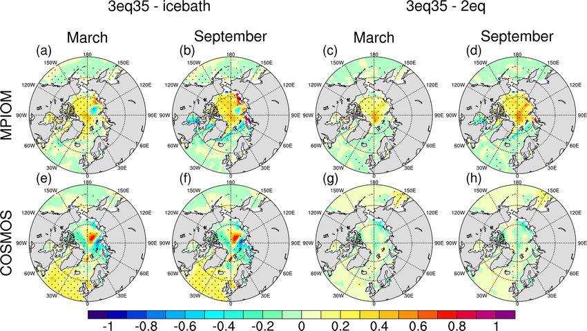
4896                                                                                                    X. Shi et al.: Ice–ocean heat flux

Table 1. List of experiments. Note that R = αh /αs denotes the ratio between turbulent exchange coefficients for heat (αh ) and salt (αs ).

      Name                 Parameterization                Tinterface                Tf                                      length
                                                                                                                             (model year)
      SIM-icebath          ice bath                        same as Tf                −1.84 ◦ C                               100
      SIM-2eq              two-equation                    same as Tf                −1.84 ◦ C                               100
      SIM-3eq35            three-equation, with R = 35     from Eqs. (1), (3), (5)   −1.84 ◦ C                               100
      SIM-3eq70            three-equation, with R = 70     from Eqs. (1), (3), (5)   −1.84 ◦ C                               100
      CICE-icebath         ice bath                        same as Tf                −1.84 ◦ C                               100
      CICE-2eq             two-equation                    same as Tf                −1.84 ◦ C                               100
      CICE-3eq35           three-equation, with R = 35     from Eqs. (1), (3), (5)   −1.84 ◦ C                               100
      MPIOM-icebath        ice bath                        same as Tf                freezing point of the uppermost cell    1000
      MPIOM-2eq            two-equation                    same as Tf                freezing point of the uppermost cell    1000
      MPIOM-3eq35          three-equation, with R = 35     from Eqs. (1), (3), (5)   freezing point of the uppermost cell    1000
      COSMOS-icebath       ice bath                        same as Tf                freezing point of the uppermost cell    1000
      COSMOS-2eq           two-equation                    same as Tf                freezing point of the uppermost cell    1000
      COSMOS-3eq35         three-equation, with R = 35     from Eqs. (1), (3), (5)   freezing point of the uppermost cell    1000

5.1    Influence of u∗ , hmix and ice concentration                       absorbed by open water is primarily used for sea ice melting,
                                                                          while in SIM-icebath no more sea ice exists, such that the
We start with a number of sensitivity experiments with our                entire heat flux into the ocean causes a warming of the sea-
simple 1-D model that were carried out to understand the un-              water. The slower melting of the ice in SIM-2eq and SIM-3eq
derlying relationship between simulated ice thickness and the             and the resulting lower heat storage in the ocean throughout
three different parameterizations. We performed four differ-              summer results in an earlier onset of sea ice formation during
ent simulations with our simple model, which in the follow-               autumn.
ing are called SIM-icebath, SIM-2eq, SIM-3eq35, and SIM-                     For SIM-icebath and SIM-2eq, the temperature at the ice–
3eq70, where for the three-equation setup the last number                 ocean interface is constant at the freezing point of the seawa-
denotes the value of R = αh /αs . We run the simulations un-              ter, which for our choice of Sseawater = 34 g kg−1 is around
til the ice reaches its equilibrium thickness, with no more               −1.84 ◦ C. For SIM-3eq, the interface temperature can be sig-
changes from one year to the next.                                        nificantly above this value, as the interface freshens through
   In our standard SIM simulations we applied u∗ =                        the melting of the comparably fresh sea ice (Fig. 1d).
0.002 m s−1 , a sea ice concentration C = 85 %, an albedo of                 Comparing SIM-2eq, SIM-3eq35, and SIM-3eq70, we
seawater αoce = 0.1 and a mixed-layer depth hmix = 40 m.                  find that the ice thins earlier and faster in SIM-2eq because
The sea ice salinity is kept at 0. In winter, when the ocean              the ocean heat flux between the ocean and the ice is amplified
loses energy to the atmosphere through the open-water part                in this setup, owing to the constantly cold interfacial temper-
of the grid cell, the simulated heat loss from the ocean is               ature. Accordingly, the oceanic temperature increases more
identical in the four setups (Fig. 1c), since their open-water            slowly throughout spring in SIM-2eq. In SIM-3eq70, the
part is identical and the ocean is constantly at its freezing             transport of salt to the interface is lower than in SIM-3eq35.
temperature (Fig. 1b). Hence, any heat that is extracted from             Hence, the interface remains fresher and warmer throughout
the mixed layer directly causes ice growth, which explains                summer. Despite the warmer interface, stronger heat fluxes
the very similar accretion rates of the sea ice (Fig. 1a). Major          and slightly faster ablation of the ice are simulated, mainly
differences between the simulations arise as soon as the net              resulting from a higher turbulent heat exchange coefficient
heat flux becomes positive and begins to heat the ocean. All              αh , which is 0.0095 in SIM-3eq35 and 0.0135 in SIM-3eq70.
energy that enters the ocean is then directly used to melt the               To quantify the different response of the simulated sea ice
ice in SIM-icebath, while some of the heat is stored in the               cover for a larger range of forcing conditions, we carried out
ocean in SIM-2eq and SIM-3eq. Hence, ice in SIM-2eq and                   a series of sensitivity studies. For each of these, we varied
SIM-3eq melts slower than the ice in SIM-icebath, and the                 one of the forcing parameters and analyzed the difference
ocean remains warmer throughout spring (Fig. 1b). Once the                in annual mean ice–ocean heat flux between SIM-3eq35 and
ice in SIM-icebath is melted completely, the ocean temper-                SIM-icebath.
ature rises rapidly and quickly exceeds that in SIM-2eq and                  We find that in our simplified setup, differences in ice
SIM-3eq. This can be explained by two facts: (1) in SIM-2eq               thickness between SIM-3eq35 and SIM-icebath increase
and SIM-3eq, the sea ice reflects most of the incoming short-             with mixed-layer depth. This is due to the fact that the same
wave radiation, and (2) in SIM-2eq and SIM-3eq the heat flux

Geosci. Model Dev., 14, 4891–4908, 2021                                                      https://doi.org/10.5194/gmd-14-4891-2021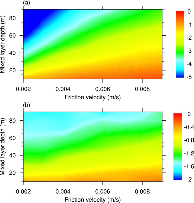
X. Shi et al.: Ice–ocean heat flux                                                                                                   4897

                                                                        Figure 2. Anomalies of ocean-to-ice heat flux in SIM for (a) three-
                                                                        equation minus icebath and (b) three-equation minus two-equation
                                                                        for different choices of mixed-layer depth and friction velocity
                                                                        (units: W m−2 ).
Figure 1. Time series of (a) sea ice thickness (m); (b) ocean temper-
ature (◦ C); (c) ocean-to-ice heat flux (W m−2 ); and (d) ice–ocean
interface temperature (◦ C) in the experiments SIM-icebath, SIM-        5.2   Ice thickness
2eq, SIM-3eq35, and SIM-3eq70 with friction velocity at 0.002 and
ice concentration at 75 %. The model is run into equilibrium.           Having understood some of the qualitative impact of the dif-
                                                                        ferent parameterizations, we can now turn to an analysis of
                                                                        their impact in the more realistic setting provided by CICE,
amount of heat input causes a smaller temperature change for            MPIOM, and COSMOS. In these models R = 35 is applied
a deeper mixed layer. According to Eq. (3), a smaller temper-           in the full three-equation approach. The presented results fo-
ature change then leads to a smaller change in heat flux to the         cus on the Arctic Ocean, as we only find a small response of
ice bottom (Fig. 2).                                                    Southern Ocean properties to the change of ice–ocean heat
   In addition, we find that the difference in sea ice thickness        flux parameterizations, in particular in MPIOM and COS-
generally decreases with friction velocity. This is related to          MOS; furthermore, the stand-alone sea ice model CICE sim-
the fact that for larger friction velocity more heat is trans-          ulates an unrealistic distribution of sea ice in warm months
ported to the ice–ocean interface in the three-equation setup           in the Southern Ocean, as it fails to capture the heat release
(Fig. 2), which enhances sea ice melt.                                  from the relatively deep mixed layer.
   Finally, regarding sea ice concentration, we find in our                We let all models run until the modeled ice cover and,
simplified setup that differences in ice thickness between              in MPIOM and COSMOS the deep-ocean temperatures,
SIM-3eq35 and SIM-icebath are larger for a smaller ice con-             reached quasi-equilibrium. More concretely, we performed
centration. This is related to the fact that the residual energy,       CICE experiments for 100 model years, with the last 10 years
which mainly comes from the net incoming heat flux through              representing its quasi-equilibrium state. For MPIOM and
open water, is all used for ablating sea ice in SIM-icebath,            COSMOS, 1000-model-year experiments were conducted,
while in SIM-3eq35 only a fraction of the heat is used for ice          and data from the last 100 model years were used for analy-
ablation. Lower ice concentration enhances the energy in the            sis. The significance level of any differences between the in-
open water and therefore also the difference in the amount of           dividual simulations was calculated by performing Student’s
heat transferred to the ice cover.                                      t test, which is used to examine if results from two differ-
                                                                        ent parameterizations are significantly different. For the Stu-
                                                                        dent’s t test, the interannual variances of the last 100 simula-
                                                                        tion years (10 years in the case of CICE) are considered.

https://doi.org/10.5194/gmd-14-4891-2021                                                   Geosci. Model Dev., 14, 4891–4908, 2021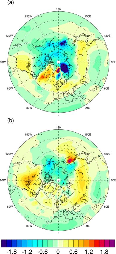
4898 X. Shi et al.: Ice–ocean heat flux
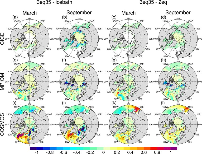
We find that the ice thickness responds similarly to the areas of Hudson Bay, Baffin Bay, the Norwegian Sea, and the
different parameterizations as it does in the simple one- Barents Sea (Fig. 5f, h). The most intriguing feature found in
dimensional model. Everything else unchanged, compared COSMOS is a significant cooling across the North Atlantic
to the three-equation approach the ice bath parameterization Ocean in the ice bath and two-equation parameterizations
leads to thinner ice throughout the Arctic Ocean both in win- compared to the three-equation approach (Fig. 5i–l). Such
ter and summer (Fig. 3). The change is similar but less pro- cooling is a consequence of weakened thermohaline circula-
nounced in the simulations based on the two-equation pa- tion, which tends to bring relatively warmer water from the
rameterization. The most significant changes occur in the lower latitudes (see Sect. 4.4).
marginal ice zone where sea ice concentration is lowest, Because brine is released from sea ice during its forma-
again consistent with the results from the one-dimensional tion and growth, the changes in ice thickness between differ-
model. In the Arctic, the change in March thickness is gener- ent parameterizations should trigger changes in upper-ocean
ally less pronounced than the change in September thickness. salinity. Indeed, we find such changes to occur (Fig. 6). In
This is due to the fact that the air-to-ocean heat flux tends to regions in which the ice bath approach or the two-equation
be negative (the ocean loses heat to the air) in March and approach cause an increased heat flux to the ice underside,
because both the temperature of the water and the temper- and hence a larger melting rate of sea ice in summer and
ature at the ice–ocean interface are maintained at the freez- a smaller growth rate in winter, the ocean is generally less
ing point. Hence, in all parameterizations the extracted heat salty in the simulations with a simplified parameterization
is directly transferred into sea ice formation. In September, of ice–ocean heat exchange than in the simulations with the
in contrast, the ocean can maintain a temperature above the full three-equation parameterization. Interestingly, the oppo-
freezing temperature in the two-equation or three-equation site sign is observed in the Barents Sea and its adjacent re-
approach but not in the ice bath approach. Hence, as in the gions (Fig. 6e–f), despite the larger melt rates in the ice bath
simple 1-D model, differences between the different param- scheme. The North Atlantic Ocean experiences a pronounced
eterizations are more pronounced during summer. freshening in the ice bath approach in COSMOS (Fig. 6e–f),
In addition, sea ice concentration is high throughout which lowers the efficiency of deep-water formation. No sig-
March, which reduces the direct interaction of atmospheric nificant differences in upper ocean salinity are found between
heat fluxes with the ocean. As discussed in the previous sub- experiments COSMOS-2eq and COSMOS-3eq35 (Fig. 6g–
section, this limits differences between the different parame- h).
terizations during wintertime. Finally, the ice thins somewhat
less in winter because of dynamical effects: the thinner ice is 5.4 Thermohaline structure of the ocean
more mobile and more prone to ridging, which fosters the
formation of areas with open water. In these areas, signifi- We now turn to the large-scale changes in the thermoha-
cant amounts of new ice can form, which dampens some of line structure of the ocean. We find that compared to the
the thermodynamic thinning of the ice pack. more realistic three-equation approach, the ice bath and
In summer, among the three parameterizations only the two-equation approaches lead to significant cooling of the
three-equation approach can result in an ice–ocean interface ocean’s deep-water masses (Fig. 7c, e, g). This behavior is
temperature above the freezing point of the uppermost ocean due to the fact that the heat flux out of the ocean is slowed
layer (Fig. 4), which reduces the ocean-to-ice heat flux. This down in the three-equation approach. Hence, more heat can
is due to the fact that the ice–ocean interface is usually very be stored in the mixed layer and further advected into the
fresh, owing to the ablation of the ice bottom. When the tem- deep ocean. However, the opposite is found in experiment
perature of the interface exceeds that of the mixed layer, a MPIOM-icebath, which results in a pronounced warming in
reversed heat flux from the ice to the ocean can occur. the deep-water masses by up to 0.5 ◦ C (Fig. 7a). This warm-
ing in the simulations with the least realistic parameterization
5.3 Upper-ocean temperature and salinity of ice–ocean heat exchange reflects the earlier ice loss in the
marginal ice zone, which causes enhanced surface warming
We now move on to analyze how the described changes in sea of the water there.
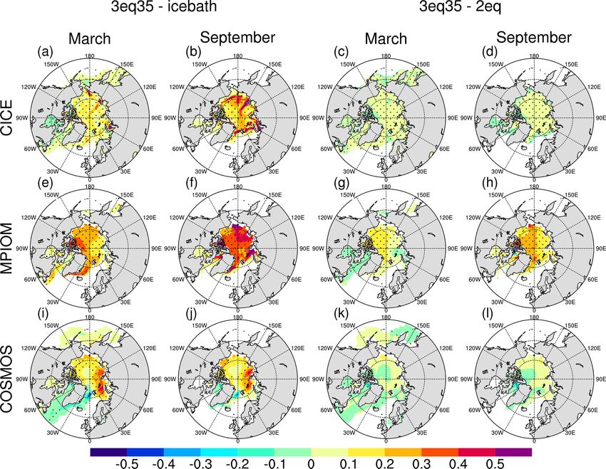
ice impact upper-ocean temperature and salinity. We find for As the simplified parameterizations both lead to faster
the Arctic Ocean that the ice bath parameterization and the melting of sea ice in the Arctic Ocean in summer and less
two-equation approach result in almost the same temperature growth in winter as compared to the most realistic approach,
distribution during winter as the more realistic three-equation one would expect a freshening of the ocean mixed layer and
approach in CICE and MPIOM (Fig. 5a, c, e, g). During sum- the deep-water mass that originates from such fresher sur-
mer, however, the ice bath approach causes warmer water to face source water. However, we find that such freshening in
persist around the ice edge in CICE (Fig. 5b). This is caused MPIOM occurs only within the Arctic upper ocean between
by the fact that here the ice melts earlier than in the three- depths of 0 and 100 m (Fig. 7b, d). In COSMOS, the fresh-
equation approach, which then allows the ocean to absorb ening extends to the bottom of the Arctic Ocean (Fig. 7f, h).
heat more efficiently. The same is found in MPIOM in the This different model behavior is currently not understood.
Geosci. Model Dev., 14, 4891–4908, 2021 https://doi.org/10.5194/gmd-14-4891-2021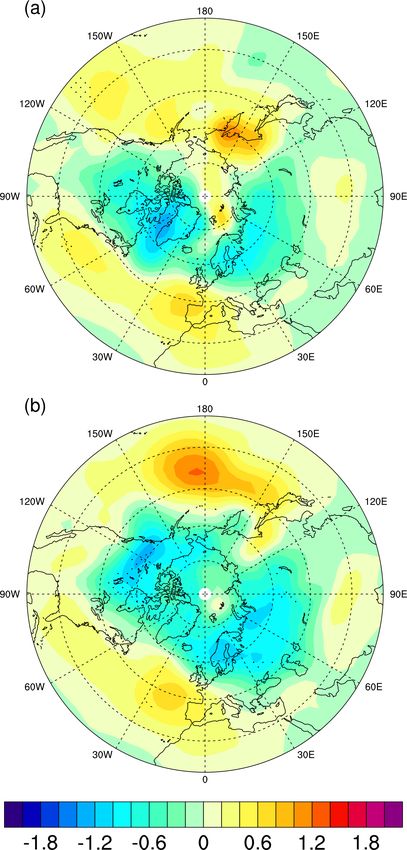
X. Shi et al.: Ice–ocean heat flux                                                                                      4899

Figure 3. The difference in the Arctic sea ice thickness for (a) CICE-3eq35−CICE-icebath in March, (b) CICE-3eq35−CICE-icebath
in September, (c) CICE-3eq35−CICE-2eq in March, (d) CICE-3eq35−CICE-2eq in September, (e) MPIOM-3eq35−MPIOM-icebath in
March, (f) MPIOM-3eq35−MPIOM-icebath in September, (g) MPIOM-3eq35−MPIOM-2eq in March, (h) MPIOM-3eq35−MPIOM-2eq
in September, (i) COSMOS-3eq35−COSMOS-icebath in March, (j) COSMOS-3eq35−COSMOS-icebath in September, (k) COSMOS-
3eq35−COSMOS-2eq in March, and (l) COSMOS-3eq35−COSMOS-2eq in September. The marked area has a significance level of greater
than 95 % based on Student’s t test (units: m).

   The Atlantic meridional overturning circulation (AMOC)        and COSMOS-2eq, respectively (Table 2). In COSMOS-
streamfunction, defined as the zonally integrated transport      icebath, the reduced sea surface salinity in the Atlantic
over the Atlantic basin, shows a weakening over 40–60◦ N,        section (Fig. 6e–f, Fig. 7f) lowers the efficiency of deep-
0–3000 m depth in MPIOM-icebath and MPIOM-2eq com-               water formation, resulting in a weakening of the AMOC
pared to MPIOM-3eq35. In COSMOS, a pronounced weak-              (Fig. 8c). A similar but less pronounced pattern is obtained
ening of AMOC is obtained south of 60◦ N. The AMOC in-           by COSMOS-2eq (Fig. 7h). No significant anomaly in the
dex, i.e., the maximum value of the AMOC streamfunction          AMOC index is found in MPIOM (Table 2).
over the region of 800–2000 m depth at 20–90◦ N, is found
to be 20.2 and 17.6 Sv in MPIOM-3eq35 and COSMOS-                5.5   Atmospheric responses
3eq35, respectively (Table 2). The latter is consistent with
the estimates of global circulation from hydrographic data       We now finally turn to investigate how the sea ice changes
(15 ± 3 Sv) (Ganachaud and Wunsch, 2000). Compared to            affect the atmospheric properties in the fully coupled model
the corresponding three-equation approach, the strength of       COSMOS.
the AMOC decreases by 1 and 0.8 Sv in COSMOS-icebath

https://doi.org/10.5194/gmd-14-4891-2021                                           Geosci. Model Dev., 14, 4891–4908, 2021
4900                                                                                                 X. Shi et al.: Ice–ocean heat flux

Figure 4. The anomaly of the Arctic ice–ocean interface temperature in (a)–(b) CICE-3eq35, (c)–(d) MPIOM-3eq35, and (e)–(f) COSMOS-
3eq35 relative to freezing point of the far-field ocean (about −1.8◦ ). The left column is for March, and the right column is for September
(units: K).

   The response in surface air temperature, as shown in                 resulting in more heat flux absorbed by the surface. (2)
Fig. 9, indicates a general warming over the Arctic Ocean               The decline of AMOC in experiments COSMOS-icebath and
and its adjacent continents in the COSMOS-icebath and                   COSMOS-2eq weakens the northward heat transport from
COSMOS-2eq compared to COSMOS-3eq35; a cooling can                      lower latitudes to North Atlantic regions. (3) The atmo-
be found for the Greenland Sea, Nordic Sea, North Atlantic              spheric circulation also plays a role, which is discussed in
Ocean, southeastern North America, and midlatitude Eura-                the following.
sia. There are various reasons responsible for these changes:              Figure 10 depicts the responses in boreal winter sea level
(1) reduced Arctic sea ice mass in the ice bath and two-                pressure (SLP). Compared to the most realistic parameteri-
equation approaches lead to a decrease in the surface albedo,           zation, the simplified approaches illustrate a more negative

Geosci. Model Dev., 14, 4891–4908, 2021                                                  https://doi.org/10.5194/gmd-14-4891-2021
X. Shi et al.: Ice–ocean heat flux                                                                                              4901

Figure 5. As in Fig. 3 but for the sea surface temperature (units: K).

Table 2. AMOC index.                                                     tive NAO mode leads to a warming over much of Europe and
                                                                         far downstream as the wintertime enhanced westerly flow
         Experiment             AMOC index       NP index                across the North Atlantic moves relatively warm and moist
         MPIOM-icebath                   20.1            –               maritime air to that region (Fig. S2a). Another notable fea-
         MPIOM-2eq                       20.2            –               ture is the cooling and warming over North Africa and North
         MPIOM-3eq35                     20.2            –               America, respectively, which is associated with the stronger
                                                                         clockwise flow around the subtropical Atlantic high-pressure
         COSMOS-icebath                  16.6       1017.5
                                                                         center. These described patterns are consistent with the mod-
         COSMOS-2eq                      16.8       1017.4
         COSMOS-3eq35                    17.6       1017.9               eled surface air temperature response over Northern Hemi-
                                                                         sphere continents (Fig. 9).
                                                                            Another intriguing pattern in the atmosphere is an anoma-
                                                                         lous negative SLP over the North Pacific Ocean in the sim-
                                                                         plified parameterizations compared to the most realistic ap-
North Atlantic Oscillation (NAO) mode, with positive SLP
                                                                         proach. Here we calculate the North Pacific (NP) index as
anomalies over the Greenland and Nordic seas and nega-
                                                                         the area-weighted SLP over the region of 30–65◦ N, 160◦ E–
tive anomalies over the North Atlantic subtropical zone. SLP
                                                                         140◦ W during boreal winter (Trenberth and Hurrell, 1994).
anomalies in another time window show a similar pattern
                                                                         The NP index in COSMOS-3eq35 is shown to be 0.4–0.5 hPa
(Fig. S1), indicating the robustness of the NAO signal in
                                                                         higher than its counterparts (Table 2). A high NP index leads
the simplified approaches even though the significance level
                                                                         to a warming over southern North America and northern
does not exceed 95 %. Composite analysis shows that a posi-

https://doi.org/10.5194/gmd-14-4891-2021                                                  Geosci. Model Dev., 14, 4891–4908, 2021
4902 X. Shi et al.: Ice–ocean heat flux
Figure 6. As in Fig. 3e–l but for the sea surface salinity (units: g kg−1 ).
Eurasia, as well as a cooling over northern North America son, we also show the distribution of mixed-layer depth in
(Fig. S2b), resembling the pattern of the surface air tempera- MPIOM-3eq35 in Fig. S3, which indicates a different lo-
ture anomalies (Fig. 9). Therefore, the response of the surface cation of the main deep-water convection site to our ice–
air temperature in the simplified parameterizations can be at- ocean coupled model: the northeastern North Atlantic. The
tributed to the combined effect of the weakened AMOC and results from the composite analysis shown in Fig. 11b indi-
NAO and the enhanced Aleutian Low. cate that the anomalous NAO pattern can lead to significant
changes in the ocean circulation. We find that the intensity
5.6 Air–sea interaction of the Labrador Sea convection is characterized by variations
that appear to be synchronized with variabilities in the NAO.
In this section the mechanism explaining the weakening Therefore, the weakening of AMOC in our simplified setups
AMOC in COSMOS-icebath and COSMOS-2eq as com- compared to the most realistic approach can be attributed to
pared to COSMOS-3eq35 is explored. It has long been rec- the simulated anomalous negative NAO phase.
ognized that the NAO variability has an important influence The NAO affects the seawater convection mainly via mod-
on the AMOC (Curry et al., 1998; Delworth and Zeng, 2016). ifying the surface heat fluxes, which leads to anomalies in
Variations in the NAO have been hypothesized to play a role the spatial and vertical density gradient. Figure 12a shows
in AMOC variations by modifying air–sea fluxes of heat, wa- the composite map between surface heat flux anomalies and
ter, and momentum. A similar relationship between NAO and the NAO index. During the positive phase of NAO, more heat
the AMOC has also been reported for past climate conditions than usual is removed from the ocean to the atmosphere in the
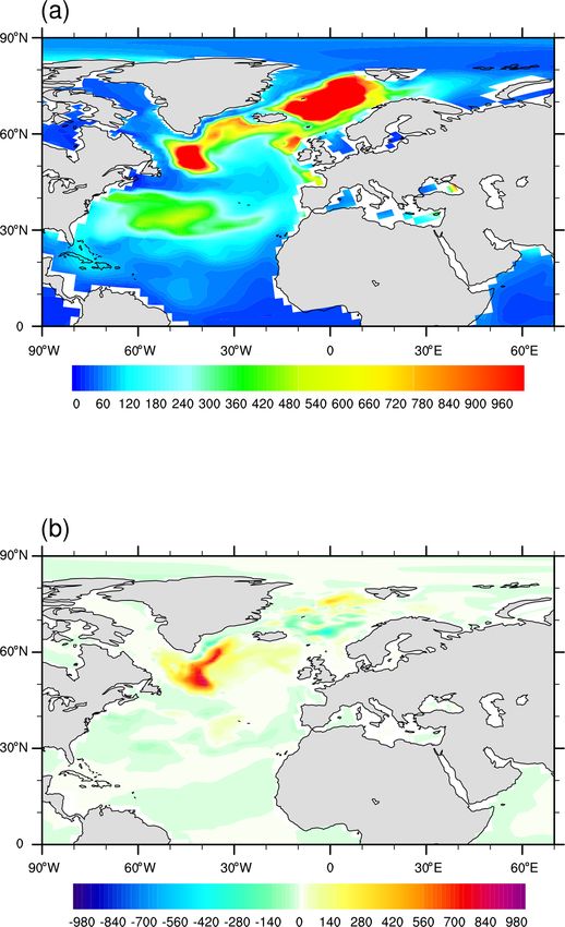
(Shi and Lohmann, 2016; Shi et al., 2020). Here in Fig. 11 western Atlantic, in particular from the Labrador Sea. Such a
we show the results from a composite analysis between the pattern is in good agreement with the NAO-relative heat flux
NAO index and the anomalies in mixed-layer depth based on anomalies derived from the European Centre for Medium-
COSMOS-3eq35. It is calculated by averaging March mixed- Range Weather Forecasts (ECMWF) interim reanalysis (Del-
layer depth anomalies (departure from the mean state) during worth and Zeng, 2016). The enhanced removal of heat favors
years when the NAO index exceeds 1 standard deviation. an increase in the surface density and thereby strengthens
The convective activities in the Labrador Sea and the deep-water formation. On the other hand, the NAO also af-
Greenland–Iceland–Norwegian (GIN) seas are shown to fects the net precipitation over the North Atlantic Ocean. As
have important contributions to the production and trans- illustrated in Fig. 12b, relatively dry condition could occur
port of North Atlantic deep water (Fig. 11a). For compari-
Geosci. Model Dev., 14, 4891–4908, 2021 https://doi.org/10.5194/gmd-14-4891-2021X. Shi et al.: Ice–ocean heat flux 4903
Figure 7. Anomalies in zonal mean temperature and salinity vertical profile across the North Atlantic section (−80–0◦ W) for the latitudes
from 30◦ S to 90◦ N (a, b) MPIOM-3eq35−MPIOM-icebath, (c, d) MPI-3eq35−MPI-2eq, (e, f) COSMOS-3eq35−COSMOS-icebath, and
(g, h) COSMOS-3eq35−COSMOS-2eq. The left column is for temperature, and the right column is for salinity (units: K and g kg−1 ).
over Labrador Sea and Irminger Sea during positive NAO istic bulk two-equation approach with freezing temperature
years. kept at the ice–ocean interface where the ocean is allowed
to be warmer than freezing point (McPhee, 1992), and (3) a
more advanced double diffusional transport (three-equation)
6 Discussion and conclusion approach with the temperature at the ice–ocean interface cal-
culated based on the melting rate of the ice bottom (Notz
In the present study, we perform 1-D simulations with an et al., 2003).
idealized columnar model (SIM), as well as global simu- The conclusions drawn from these models in terms of sea
lations with a stand-alone sea ice model (CICE), an ice– ice properties are quite similar to each other. The thinnest ice
ocean coupled model (MPIOM), and a fully coupled climate is observed in the ice bath simulations, as no residual heat is
model COSMOS, to analyze the sensitivity of modeled cli- allowed to remain in the ocean and the seawater beneath sea
mate to ice–ocean interface heat flux parameterizations. This ice is constantly at its freezing point. The two-equation ex-
is achieved by implementing the following elements into the periments simulate thicker sea ice because some of the heat
models: (1) a simple ice bath assumption with the ocean tem- is stored in the ocean rather than used for ablating the ice.
perature fixed at the freezing temperature, (2) a more real-
https://doi.org/10.5194/gmd-14-4891-2021 Geosci. Model Dev., 14, 4891–4908, 20214904 X. Shi et al.: Ice–ocean heat flux Figure 8. Anomalies in AMOC (a) MPIOM-3eq35−MPIOM-icebath, (b) MPI-3eq35−MPI-2eq, (c) COSMOS-3eq35−COSMOS-icebath, and (d) COSMOS-3eq35−COSMOS-2eq (units: Sv). The simulated sea ice by the three-equation approach has In contrast to their and other previous studies, in our study the largest thickness, as the temperature at the ice–ocean in- we do only use a stand-alone sea ice model but also analyze a terface can exceed the freezing point of the far-field ocean, coupled ice–ocean model and an Earth system model. These causing the heat flux from the ocean to be reduced or even allow us to examine the effect of various oceanic heat flux reversed. The marginal ice areas are found to be highly sen- formulations on the deep ocean and atmospheric circulation, sitive to the choice of ice–ocean heat flux parameterizations. as well as their impact on sea ice properties. In our study, In particular, the seawater temperature in the marginal ice COSMOS reveals intensification in both the AMOC and zones is largely determined by the onset or retreat of the sea NAO when the most advanced ice–ocean heat flux param- ice. eterization is applied. Ocean observations and model simu- As a result of the brine release during sea ice formation, lations show that the changes in the thermohaline circulation the Arctic Ocean is most salty in the three-equation experi- during the last century have been driven by low-frequency ment and least salty in the ice bath experiment. The same is variations in the NAO via changes in Labrador Sea convec- found in the deep-water masses due to their coupling with the tion (Latif et al., 2006). More recently, a delayed oscillator surface source water. The thermohaline instability obtained model and a climate model suggest that the NAO forces the from such a salinity profile is responsible for a strengthening AMOC on a 60-year cycle (Sun et al., 2015). The strength- of the Atlantic meridional overturning circulation (AMOC) ening of the AMOC, obtained in our COSMOS-3eq experi- in the coupled simulation with the three-equation approach. ment, is likely due to the combined effect of increased ther- Note that our results are in good agreement with a previous mohaline instability and the anomalous NAO+ mode. In con- study using CICE (Tsamados et al., 2015) that found stronger trast, no obvious response of the AMOC can be found in the basal melting of Arctic sea ice, decreased Arctic Ocean salin- MPIOM experiments (Table 2). As indicated in the present ity, cooling of seawater in the central Arctic, and warming paper and many other studies (Curry et al., 1998; Latif et al., of seawater at the ice edge in the two-equation experiments 2006; Sun et al., 2015), the AMOC is closely related to the compared to the three-equation approach in August. How- atmospheric processes over the North Atlantic Ocean. One of ever, in their study the effects are more pronounced, possibly the key elements controlling the atmospheric circulation over because we used different model versions of CICE and differ- the North Atlantic is the NAO. As the atmospheric forcings ent parameters for the ice–ocean heat flux formulations: one are prescribed in MPIOM, there is no difference in the at- example is the value for R, which is 50 in Tsamados et al. mospheric state among the MPIOM experiments. Therefore, (2015) and 35 in our case. In addition, different atmospheric the prescribed atmospheric forcing largely limits the air–sea forcings were used in the two studies. interaction feedback. Geosci. Model Dev., 14, 4891–4908, 2021 https://doi.org/10.5194/gmd-14-4891-2021
X. Shi et al.: Ice–ocean heat flux                                                                                   4905

                                                              Figure 10. Anomalies in boreal winter sea level pressure
                                                              (a) COSMOS-3eq35−COSMOS-icebath, and (b) COSMOS-
Figure 9. Anomalies in surface air temperature (a) COSMOS-    3eq35−COSMOS-2eq (units: hPa).
3eq35−COSMOS-icebath and (b) COSMOS-3eq35−COSMOS-
2eq (units: K).

                                                              Lohmann, 2007; Parker et al., 2007). The AMOC-induced
                                                              warming helps to reduce the sea ice mass over the Arctic and
   Our study indicates a less pronounced sea ice response     North Atlantic subpolar regions. Indeed, the sea ice across
to ice–ocean interface heat flux parameterizations in the     the Greenland Sea and Baffin Bay are found to be thinnest in
fully coupled climate model COSMOS than in the ice–ocean      COSMOS-3eq.
model MPIOM (compare Fig. 3e–h with Fig. 3i–l). This is          It should be noted that CICE is in many aspects differ-
because the change of the AMOC has a dampening effect         ent from the sea ice component in MPIOM. (1) CICE uses
on the simulated sea ice anomalies. The strengthening of      the multi-layer approach with a sub-grid-scale ice thickness
the AMOC in COSMOS-3eq can lead to a warming over             distribution (Bitz and Lipscomb, 1999), while MPIOM uses
the Northern Hemisphere, especially over the North Atlantic   zero-layer thermodynamics following Semtner Jr. (1976). (2)
and the Arctic. This hypothesized link between the AMOC       A submodel of ice dynamics based on an elastic–viscous–
and Northern Hemisphere mean surface climate has been         plastic rheology (Hunke and Dukowicz, 1997; Hunke, 2001)
documented in an abundance of studies (e.g., Schlesinger      is used in CICE, while in MPIOM viscous–plastic dynam-
and Ramankutty, 1994; Rühlemann et al., 2004; Dima and        ics following Hibler III (1979) are used. (3) Different spa-

https://doi.org/10.5194/gmd-14-4891-2021                                       Geosci. Model Dev., 14, 4891–4908, 2021
You can also read