Spatiotemporal Varying Effects of Built Environment on Taxi and Ride-Hailing Ridership in New York City
←
→
Page content transcription
If your browser does not render page correctly, please read the page content below
International Journal of
           Geo-Information

Article
Spatiotemporal Varying Effects of Built Environment
on Taxi and Ride-Hailing Ridership in New York City
Xinxin Zhang 1 , Bo Huang 2, * and Shunzhi Zhu 1
 1    College of Computer and Information Engineering, Xiamen University of Technology, Xiamen 361024, China;
      zhangxinxin@xmut.edu.cn (X.Z.); szzhu@xmut.edu.cn (S.Z.)
 2    Department of Geography and Resource Management and Institute of Space and Earth Information Science,
      The Chinese University of Hong Kong, Hong Kong 999077, China
 *    Correspondence: bohuang@cuhk.edu.hk

 Received: 18 June 2020; Accepted: 27 July 2020; Published: 29 July 2020

 Abstract: The rapid growth of transportation network companies (TNCs) has reshaped the traditional
 taxi market in many modern cities around the world. This study aims to explore the spatiotemporal
 variations of built environment on traditional taxis (TTs) and TNC. Considering the heterogeneity of
 ridership distribution in spatial and temporal aspects, we implemented a geographically and
 temporally weighted regression (GTWR) model, which was improved by parallel computing
 technology, to efficiently evaluate the effects of local influencing factors on the monthly ridership
 distribution for both modes at each taxi zone. A case study was implemented in New York City
 (NYC) using 659 million pick-up points recorded by TT and TNC from 2015 to 2017. Fourteen
 influencing factors from four groups, including weather, land use, socioeconomic and transportation,
 are selected as independent variables. The modeling results show that the improved parallel-based
 GTWR model can achieve better fitting results than the ordinary least squares (OLS) model, and it
 is more efficient for big datasets. The coefficients of the influencing variables further indicate that
 TNC has become more convenient for passengers in snowy weather, while TT is more concentrated at
 the locations close to public transportation. Moreover, the socioeconomic properties are the most
 important factors that caused the difference of spatiotemporal patterns. For example, passengers
 with higher education/income are more inclined to select TT in the western of NYC, while vehicle
 ownership promotes the utility of TNC in the middle of NYC. These findings can provide scientific
 insights and a basis for transportation departments and companies to make rational and effective use
 of existing resources.

 Keywords: geographically and temporally weighted regression; taxi; Uber; spatiotemporal analysis

1. Introduction
     With the popularity of mobile phone usage, transportation network companies (TNCs) that offer
app-based services, such as Uber, DiDi, and Lyft, claim to provide stability and convenience with
peer-to-peer (p2p) processes that connect passengers and private drivers on-line and in real-time [1].
As an emerging form of transportation based on network and mobile technology, the analysis of TNC
ridership has become a hot topic in urban transportation research. Much evidence has shown that
the rapid development of TNC has had a huge impact on the traditional taxi (TT), leading the taxi
industry to experience significant losses in terms of market share, revenue, labor power and facility [2].
This is particularly obvious in large modern cities such as New York City (NYC), where the annual taxi
load decreased from 145 million in 2015 to 113 million in 2017, decreasing nearly 23% in three years.
In contrast, the ridership by TNCs increased from 37 million to 110 million. The reduction in the
market share of the taxi industry will inevitably cause a decline in the income of taxi drivers and the

ISPRS Int. J. Geo-Inf. 2020, 9, 475; doi:10.3390/ijgi9080475                        www.mdpi.com/journal/ijgi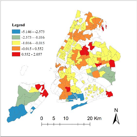
ISPRS Int. J. Geo-Inf. 2020, 9, 475                                                                  2 of 23

compression of the taxi business scale, leading to economic difficulties and even the bankruptcy of taxi
companies. In May 2013, although the price of a yellow car’s license plate in NYC had been cut in half,
the licenses of many taxi company vehicles were idle because of the lack of new drivers [3].
       Nevertheless, many researchers insist that it is premature to announce the inevitable demise of the
taxi industry based on the current success of TNC. For example, Wang et al. reported that the success
of TNCs lies in an aggressive but unsustainable price subsidy strategy [4]. Cramer and Krueger’s
study [5] observed that most trips on TNC are concentrated in daily traffic peak periods. Regarding
off-peak periods, traditional taxis still account for a large proportion of transportation and thus cannot
be replaced. Furthermore, according to the statistical results from [6], the average number of working
hours per week of Uber drivers was approximately half that of many taxi drivers in the U.S.
       Regardless of these debates, it is indisputable that the taxi industry is currently facing a huge
challenge and competition from the TNC in many aspects. Therefore, analysis of the differentiation of
these two modes, such as the characteristics of the target passengers and travel pattern, is conducive
to a better understanding of the competitive relationships between them. However, as all these
differentiations are not uniform within a city and are driven by diverse factors, the widely used global
statistical models are limited to incorporate the significance of spatiotemporal heterogeneity and
autocorrelation. The spatiotemporal analysis between taxi/TNC ridership and the built environment is
still an open issue.
       This paper presents the results of our research utilizing an improved GTWR model based on
parallel computation to efficiently explore the spatiotemporal relationships between TT/TNC and the
built environment in NYC, where about 659 million trips occurred from 2015 to 2017. The rest of
this paper is arranged as follows. Section 2 provides a brief review of the relevant research progress,
and Section 3 presents the details of the parallel-based GTWR model adopted in this study. Section 4
introduces the related dataset and describes how the data were processed. Section 5 mainly analyzes
the model accuracy and findings. Section 6 discusses the spatiotemporal patterns between taxi and
TNC. The last section elaborates upon the conclusions of this paper, as well as future research directions.

2. Related Literature
     Taxis have historically comprised a far lower share and geographical coverage of urban
transportation than other transport modes, such as buses and subways; therefore, there are many
lesser extensive studies on taxis than on other transport modes. In general, researchers have found
taxis to be both complements and substitutes for public transit [2]. Despite their small share in urban
transportation, taxis fill a critical gap by providing mobility service and all-day operation, which
are not available in other transportation modes. More importantly, with the popularization of GPS
auto-collection devices, the spatiotemporal characteristics of ridership and trajectory by taxis provide a
valuable reference for mining the travel patterns of citizens and for traffic optimization [7]. Therefore,
the spatiotemporal analysis of taxis has become a research hotspot in recent years.
     Early research on taxis mainly focused on market demand components based on the inherent
attributes of the taxi industry, such as price, tips, labor costs, and other factors [8]. Because the
measurement of cost, waiting time, and convenience is usually derived from investigations or relevant
departments, those data are biased and lack objectivity. With the GPS devices carried by taxis,
the spatiotemporal data of taxis can be tracked and collected in real-time. These data have the
advantage of spatial-temporal characteristics than previous data and can integrate with external
geographic factors, such as land use [9] and weather [10,11]. For example, Liu et al. used GPS data
of taxi and urban land use factors to identify ‘source-sink areas’ in Shanghai [12]. Nevertheless,
previous studies mostly adopted the ordinary least squares (OLS) method [13,14]. In the OLS model,
the aggregated pickup (PU) and drop-off (DO) locations of taxis are used as dependent variables,
and the relevant influencing factors, such as weather and land use, are selected as independent variables.
Given spatial autocorrelation and heterogeneity exists in the distribution of PU and DO locations for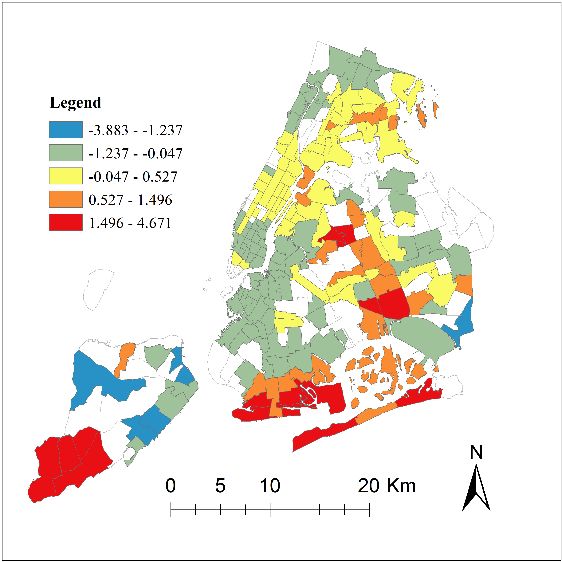
ISPRS Int. J. Geo-Inf. 2020, 9, 475                                                               3 of 23

TT and TNC, the precondition of the OLS model that the observations should be independent of each
other is difficult to satisfy.
      To address this issue, Fotheringham et al. proposed a local regression model called Geographically
Weighted Regression (GWR) [15], which improves the accuracy of regression results by constructing a
local spatial weight matrix for estimating variation in space. Furthermore, the GWR model extends the
traditional regression framework by allowing parameter estimates to vary in space and is therefore
capable to capture local effects. The GWR model has been widely applied in transit ridership
analysis [16,17]. For example, based on NYC’s taxi data, Qian et al. [18] used the GWR model to
analyze the relationship between taxi locations and urban environmental factors. The results show
that the GWR model can provide better model accuracy and interpretation than the OLS model.
One of the remaining problems is that the GWR model only obtains related variable coefficients in the
spatial dimension. While dealing with time series datasets, those data often need to be aggregated or
separated based on their timestamps, thereby ignoring the fact that the distribution of taxis or TNCs
varies with different scales of time. Recently, scholars have put forward many improved strategies to
account for both temporal and spatial variability, such as the GWR-TS [19] and linear mixed effect
(LME) + GWR models [20]; still, these models are generally based on the two-stage least squares
regression [21], first fitting the temporal effect using the LME model and then evaluating the spatial
heterogeneity effects with the GWR model. Those models cannot simultaneously consider temporal
and spatial effects.
      To simultaneously model temporal and spatial effects, Huang et al. proposed an improved
GWR-based model, named Geographical and Temporal Weighted Regression (GTWR) [22], which is
thought to design simultaneous spatial and temporal weighting. Thus, the GTWR model can reflect
continuous variations for each location at each time. The initial implementation of the GTWR model
was carried out for house-price estimation, and the results showed that the accuracy of the GTWR
model was superior to that of the OLS and GWR models. Recently, the GTWR model has been extended
in many fields, such as air quality [23] and environmental research [24]. Moreover, some scholars have
put forward improved GTWR schemes successively. For example, Wu et al. proposed an improved
model, known as the Geographically and Temporally Weighted Autoregressive (GTWAR) model,
to estimate spatial autocorrelations [25], and Du et al. proposed a Geographically and circle-Temporally
Weighted regression (GcTWR) model for enhancing the seasonal cycle of long-term observed data [26].
      The above research fully shows that the GTWR model has great advantages in spatiotemporal
modeling. Ma et al. applied the GTWR model to public transit and achieved good modeling
results [27]. Zhang et al. also adopted the GTWR model to taxi ridership analysis and achieved
a similar conclusion [28]. Nevertheless, due to the fact that the spatiotemporal nonstationarity of
taxis is more complicated than other modes of transit such as buses that have preset routes, previous
studies have generally been limited to taxis or TNC separately, and few studies take into consideration
the difference between taxis and TNC. Research on TNC remains relatively scarce, although its data
structure is similar to that of taxis. Thus, applying the GTWR model for simultaneous analysis of both
taxis and TNC is still an unsolved issue.

3. Methodology
      In this section, we briefly review the basic framework for the GTWR model and how to determine
the parameters of the GTWR model. Then, we propose a parallel computing scheme to improve the
efficiency of the GTWR model and apply the model to ridership modeling.

3.1. The Basic Framework of the GTWR Model
     The GWR-based model is a local-based spatially varying coefficient regression algorithm that
extends the OLS model by adopting local parameters to be estimated. It is capable of significantly
improving the estimation accuracy of spatial data, especially for those areas with complex spatial
nonstationarity. On this foundation, Huang et al. [22] proposed a GTWR model focusing on
ISPRS Int. J. Geo-Inf. 2020, 9, 475 4 of 23
spatiotemporal kernel function definition and spatiotemporal bandwidth optimization, which can
simultaneously address spatial and temporal nonstationarity issues. Assuming that the observation of
taxi ridership is denoted as Yi , where i (I = 1, 2, . . . , n) represents a spatial unit, such as traffic analysis
zone (TAZ), thus the GTWR model can be mathematically expressed as follows:
X
Yi = β0 (ui , vi , ti ) + βk (ui , vi , ti )Xki + εi , (1)
k
where (ui , vi , ti ) represents the center coordinates of TAZ i in a spatial location (ui , vi ) at time ti ; β0 is the
intercept value; βk (ui , vi , ti ) denotes the slope for each independent variable Xki ; and εi is the random
error. The variables Xki refer to the influencing factors that improve the associations between ridership
and urban environmental factors, such as weather, land use, socioeconomic, and transport condition.
For a given dataset, a locally weighted least squares method is usually employed to estimate the
intercept of β0 , as well as the slopes βk for each variable. The GTWR models assume that the closer to
point i in the space-time coordinate system, the greater the weight of the measurements in predicting
βk will be. Thus, the coefficients of β̂ = (β0 , β1 , .., βk )T can be estimated by:
−1
β̂(ui , vi , ti ) = [XT W(ui , vi , ti )X] XT W(ui , vi , ti )Y, (2)
where X is the n×(k+1) matrix of input variables. Y is the n-dimensional vector of the output variables.
The space-time weight matrix W(ui , vi , ti ) is an n × n weighting matrix to measure the importance
of point i to the estimated point j for both space and time. The Gaussian function is one of the most
commonly used weight function:
dij 2
Wij = exp(− 2 ), (3)
h
where dij denotes a spatiotemporal distance between points i and j, and h is a nonnegative parameter
that presents a decay of influence with distance. By combining the temporal distance dT with the
spatial distance dS , the spatiotemporal distance can be expressed as:
dST = ds ⊗ dT , (4)
where ‘⊗’ can represent different types of operators. In this study, the ‘+’ as the combination operator
was selected to calculate the total spatiotemporal distance. With respect to the different scale effects
of space and time, an ellipsoidal coordinate system was constructed to measure the spatiotemporal
distance between each regressive point and the surrounding points [29]. The spatiotemporal distance
between taxi ridership can thus be expressed as the linear weighting combination indicated below:
2 2 2 2
(dST
ij ) = λ[(ui − u j ) + (vi − v j ) ] + µ(ti − t j ) , (5)
where ti and t j denote the observed time of point i and j. λ and µ are the weights for balancing the
influences of differing units between space and time variability. The weight matrix is constructed by
using the Gaussian distance decay-based functions and Euclidean distance:
2
(dST
ij
)
Wij = exp[− hST 2
]
(6)
[(ui −u j )2 +(vi −v j )2 ]+τ(ti −t j )2
= exp{− hs 2
}
where the parameter τ stands for the non-negative parameter of scale factor calculated by µ/λ (λ , 0). hST
is a positive parameter named the spatiotemporal bandwidth. Thus, if the spatiotemporal bandwidth
and scale factor are determined, the weight matrix W (ui , vi , ti ) and β̂(ui , vi , ti ) can be obtained.ISPRS Int. J. Geo-Inf. 2020, 9, 475 5 of 23
The adjustment parameters of hST and τ can be acquired either utilizing a cross-validation (CV)
process via minimization in terms of the corrected Akaike information criterion (AICc ) [30] as follows:
X
CVRSS(h) = [ yi − y,1 (h)]2 , (7)
i
RSS(h) n + tr(H (h))
AICc (h) = n log( )+nlog(2π)+n( ), (8)
n n − 2 − tr(H (h))
where y,1 (hs ) indicates the predicted value yi from the GTWR model with a bandwidth of h. Therefore,
the selection of the optimum h can be acquired through plotting CV(h) against the parameter h.
In Equation (8), RSS is the residual sum of squares, and tr(H (h)) is the trace of the hat matrix H(h).
3.2. Implementation of GTWR for Ridership Analysis
Figure 1 presents a flowchart of the implementation using GTWR for ridership analysis. Before
constructing the GTWR model for taxi ridership analysis, the observed spatial unit and temporal
resolution must be determined first. The spatial unit is generally related to the geographic extent of the
study area, which can be divided by administrative regions or a regular cell. Due to the limitation
of TNC data obtained from NYC, the spatial unit adopted in this study was based on TAZ rather
than Zip Code Tabulation Areas (ZCTA). In terms of the temporal resolution, different resolutions,
such as yearly, monthly, daily, and hourly scales, can be adopted. Since the dataset we adopted was
from 2015 to 2017, the month was considered an appropriate minimum unit of time to reduce the
cost of computation. Using the same dataset, the OLS and GTWR models were respectively applied
to estimating
ISPRS the2020,
Int. J. Geo-Inf. globe9, x and localREVIEW
FOR PEER coefficients for both modes and their relationship with the urban
6 of 24
architecture environment.
Figure 1. The flowchart of the implementation using GTWR for ridership analysis.
Figure 1. The flowchart of the implementation using GTWR for ridership analysis.
To quantitatively evaluate the spatiotemporal variation of ridership for taxis and TNC, three
variables, including the ridership for two types of TT (yellow + green), the ridership of TNC and the
proportion of TNC (PoT = TNC/(TT+TNC)), were selected as dependent variables. With respect to
independent variables, we extracted four groups of explanatory variables from multiple openISPRS Int. J. Geo-Inf. 2020, 9, 475 6 of 23
To quantitatively evaluate the spatiotemporal variation of ridership for taxis and TNC,
three variables, including the ridership for two types of TT (yellow + green), the ridership of
TNC and the proportion of TNC (PoT = TNC/(TT+TNC)), were selected as dependent variables. With
respect to independent variables, we extracted four groups of explanatory variables from multiple
open datasets. More details about raw data processing can be found in Section 4.
Several aspects need to be adjusted when applying the GTWR model to taxi ridership analysis.
Firstly, compared with the fixed kernel function, the adaptive kernel function can adjust bandwidths
according to the density of data points. Thus, it might be a more reasonable way to obtain the weights
Wij for the irregular sharp of TAZs. For simplicity, we use the q-nearest neighbors based on the
following modified bi-square function:
2
[1 − (dij /hi )2 ] , if dij < hi
Wij = , (9)
0, otherwise
where hi stands for the different bandwidths, which express the q nearest neighbors to consider in
the estimation of regression at location i. Thus, the adjustment parameter of fixed bandwidth hST is
replaced with the number of nearest neighborhood points q. Note that the q should be constrained to
q ≥ 40, otherwise the model will suffer over-fitting problem [25].
The computation of the GTWR model is intensive because each sample uses an adaptive type of
bandwidth, which leads to (t*(n − 1)n ) combinations of possible values that must be computed for the
optimal bandwidth [15]. The computing time will exponentially increase as the number of samples
and timestamps increases by, for example, using grid-based data as the spatial unit or constructing
the daily GTWR model based on several years of data. An optimized modeling approach is needed
to reduce computation consumption. In particular, we employed parallel computing to break down
the computational loops of optimal parameter selection into independent parts with different values
of q and τ. These parts can be executed simultaneously by multiple processors communicating via
shared memory, the results of which are combined upon completion as part of the overall algorithm.
Thus, the optimal values of q and τ could be efficient found. According to the principle of GTWR,
the main computing power is consumed by iteration for obtaining both adjustment parameters.
Since the process of finding the optimal adjustment parameters is independent for each iteration,
it is suitable for parallel programming. The GTWR algorithm adopted in this study is programmed
based on Matlab® , which provides a function called fminbnd for obtaining the optimal value q and
τ. The process of parallel computing can be realized through a loop process, namely parfor [31].
The platform for efficiency comparison is based on an Inter® i7-4790 CPU, which has four cores for
parallel computing. Figure 2 shows the flow chart of GTWR model using parallel computing. To verify
the robustness of the results, different proportions of training samples were randomly selected for the
GTWR model, while the remaining samples were used for verification.Matlab®, which provides a function called fminbnd for obtaining the optimal value q and τ. The
process of parallel computing can be realized through a loop process, namely parfor [31]. The platform
for efficiency comparison is based on an Inter® i7-4790 CPU, which has four cores for parallel
computing. Figure 2 shows the flow chart of GTWR model using parallel computing. To verify the
robustness
ISPRS of2020,
Int. J. Geo-Inf. the 9,results,
475 different proportions of training samples were randomly selected for
7 of 23 the
GTWR model, while the remaining samples were used for verification.
Start
Variables:
(Y,X,east,north,t,n)
Y: Taxi & FHV
X: related factors
east: coordinate of X
north: coordinate of Y
parfor i=1 to n t: time of month
n:number of samples
using fminbnd to
estimate spatial-
temporal distance (dST)
parfor i=1 to n
finish
Weight matrix(Wij)
based on Gaussian Y,AIC,R2,RSS
Kernel
W=diag(Wij) Sum Square Total
β i(ui,vi,ti) Hat matrix(Sij) Sum Square Error
Figure 2. The flow chart of GTWR model using parallel computing.
Figure 2. The flow chart of GTWR model using parallel computing.
4. Data Preparation
4. Data Preparation
4.1. Study Area
The
4.1. study
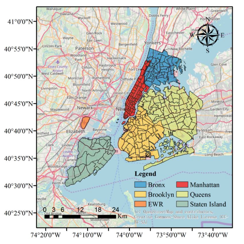
Study area of NYC consists of five boroughs, including the Bronx, Brooklyn, Staten Island,
Area
Queens, and Manhattan. As shown in Figure 3, NYC is divided into 263 taxi zones, including three
The study area of NYC consists of five boroughs, including the Bronx, Brooklyn, Staten Island,
airport zones, 55 yellow zones (only yellow cabs are allowed to pick up passengers) in Manhattan,
Queens, and Manhattan. As shown in Figure 3, NYC is divided into 263 taxi zones, including three
and 205 borough zones, in which both types of taxis are allowed to operate. TNCs are allowed in all
airport zones, 55 yellow zones (only yellow cabs are allowed to pick up passengers) in Manhattan,
areas. Previous scholars’ research [32] reported that 95% of yellow passengers are concentrated in the
and 205 borough zones, in which both types of taxis are allowed to operate. TNCs are allowed in all
Manhattan area, indicating that there were obvious imbalances in terms of spatial distribution and
areas. Previous scholars’ research [32] reported that 95% of yellow passengers are concentrated in the
emphasizing the need to establish the GTWR model.
Manhattan area, indicating that there were obvious imbalances in terms of spatial distribution and
emphasizing the need to establish the GTWR model.ISPRS
ISPRSInt.
Int.J.J.Geo-Inf. 2020,9,9,475
Geo-Inf.2020, x FOR PEER REVIEW 8 8ofof2324
Figure 3. Taxi zones of NYC (263 in total, classified in five boroughs).
Figure 3. Taxi zones of NYC (263 in total, classified in five boroughs).
4.2. Taxis and TNC Data
4.2. Taxis and TNC Data
The raw data from 2015 to 2017 were download from the NYC Taxi and Limousine Commission
(TLC, The
available
raw dataat http://www.nyc.gov/html/tlc/html/about/trip_record_data.shtml).
from 2015 to 2017 were download from the NYC Taxi and Limousine The department
Commission
provided three types
(TLC, available of data from 2009 to 2018, including two types of traditional taxis
at http://www.nyc.gov/html/tlc/html/about/trip_record_data.shtml). The(yellow and
department
green) and TNC
provided threedata,
typesinofCSV
dataformat. Eachto
from 2009 trip record
2018, on taxistwo
including included
typesthe PU and DOtaxis
of traditional timestamps
(yellowand and
locations,
green) and number of passengers,
TNC data, travel time,
in CSV format. Each travel distance,
trip record and included
on taxis price attributes.
the PUHowever, instead of
and DO timestamps
Pick-Up (PU) and
and locations, Drop-Off
number (DO) points,travel
of passengers, the TNC triptravel
time, data that was public
distance, sinceattributes.
and price 2015 only provided
However,
the taxi zones
instead due to
of Pick-Up privacy
(PU) protection.
and Drop-Off (DO) Currently,
points, the NYC
TNChastripthree
datatypical
that was taxi modes,
public sinceincluding:
2015 only
(1) yellow taxi
provided the serving
taxi zones anywhere within the
due to privacy city boundary;
protection. (2) green
Currently, NYC taxis (Borotypical
has three taxi) serving only
taxi modes,
serving city remote areas except for two airports; (3) TNC serving the same
including: (1) yellow taxi serving anywhere within the city boundary; (2) green taxis (Boro taxi) extent as yellow taxis.
Table 1 provides
serving morecity
only serving details about
remote the except
areas summary for statistics of the
two airports; (3)three
TNCtypes of taxis,
serving respectively.
the same extent as
The totaltaxis.
yellow number of recorded
Table 1 providesPUs by yellow
more detailscars
aboutwasthe
390summary
million, the total number
statistics of recorded
of the three types PUs by
of taxis,
TNCs was 212 The
respectively. million,
totaland the total
number number of
of recorded PUs recorded
by yellowPUscars
by green
was 390cars was only
million, the57 million.
total number of
recorded PUs by TNCs was 212 million, and the total number of recorded PUs by green cars was only
57 million. Table 1. Statistical description of two types of taxis and TNC data.
Type 2015 2016 2017 Total
Table 1. Statistical description of two types of taxis and TNC data.
Yellow 146,112,989 131,165,043 113,496,706 390,774,738
Type 2015
72.28% 2016
59.80% 2017
47.46% Total
59.15%
TNC
Yellow 36,910,806
146,112,989 69,131,726
131,165,043 106,676,500
113,496,706 212,719,032
390,774,738
18.26% 31.52% 44.60% 32.20%
72.28% 59.80% 47.46% 59.15%
Green 19,116,598 19,054,688 18,990,815 57,162,101
TNC 36,910,806
9.46% 69,131,726
8.69% 106,676,500
7.94% 212,719,032
8.65%
Total 18.26%
202,140,393 31.52%
219,351,457 44.60%
239,164,021 32.20%
660,655,871
Green 19,116,598 19,054,688 18,990,815 57,162,101
9.46% 8.69% 7.94% 8.65%
Due to the limitation of data security, the downloaded TNC data only included the timestamp of
Total 202,140,393 219,351,457 239,164,021 660,655,871
PU and DO and the TAZ’s ID where both coordinates were located. Therefore, to ensure the unity ofISPRS Int. J. Geo-Inf. 2020, 9, x FOR PEER REVIEW 9 of 24
ISPRS Due toGeo-Inf.
Int. J. the limitation
2020, 9, 475of data security, the downloaded TNC data only included the timestamp 9 of 23
of PU and DO and the TAZ’s ID where both coordinates were located. Therefore, to ensure the unity
of spatial reference, the taxi zone defined by TLC was adopted as the basic spatial unit, and number
ofspatial
months reference, the taxi
was selected zone
as the defined unit.
temporal by TLC was adopted as the basic spatial unit, and number of
months was selected as the temporal unit.
After determining the spatiotemporal unit, i.e., each observation represented the total number
After determining
of ridership at one taxi zone the spatiotemporal
in a certain month, unit,thei.e.,dependent
each observation
variables represented
of monthlythe total number
ridership were
of ridership at one taxi zone in a certain month, the dependent variables
derived based on the spatial and temporal aggregations of each trip. First, the raw data were of monthly ridership were
derived based on the spatial and temporal aggregations of each trip.
imported into the PostGIS spatial database. The data cleansing process was employed to excludeFirst, the raw data were imported
into the PostGIS
unavailable spatial
data (such as database. The data cleansing
missing coordinates and missing process was employed
timestamps). Then, toallexclude unavailable
PU geolocations or
data (such as missing coordinates and missing timestamps). Then, all
taxi zone ID were aggregated into 263 TAZs. Second, we count trips in the same month as monthly PU geolocations or taxi zone ID
were aggregated
ridership for everyinto TAZ. 263 TAZs. Second, we count trips in the same month as monthly ridership for
every TAZ.
Figure 4 shows the statistical PU samples for the three types of trips over 36 months. The
Figure
ridership 4 shows
operated bythe statistical
green taxis wasPU samples
small and fordecreased
the three types of trips
slightly over over
time;36 months.of
ridership The
theridership
yellow
operated by green taxis was small and decreased slightly over time;
taxis decreased at a rate of approximately 12% per year. Meanwhile, seasonal variations were also ridership of the yellow taxis
decreased at a rate of approximately 12% per year. Meanwhile, seasonal
observed, i.e., there were two peak periods from March to May and from September to November in variations were also observed,
i.e., there
every year;wereOn two peak periods
the contrary, from March
the ridership of to May grew
TNCs and from
verySeptember to November
rapidly, especially in every
in July 2017, year;
the
On the contrary,
monthly ridership theofridership
TNC firstly of TNCs grewyellow
exceeded very rapidly, especially
taxis. Finally, weinobtain
July 2017,
9120the monthly
valid ridership
observations,
of TNC
348 firstly exceeded
observations yellow taxis.
were excluded due toFinally,
no tripwe obtainAccording
record. 9120 validtoobservations,
the literature348 observations
[18], we carriedwereout
excluded due to no trip record. According to the literature [18], we carried
the log transformation for the three dependent variables to eliminate the influence of the non-normal out the log transformation
for the three dependent variables to eliminate the influence of the non-normal distribution.
distribution.
Figure 4. Monthly ridership of three types of taxis in NYC from 2015 to 2017.
Figure 4. Monthly ridership of three types of taxis in NYC from 2015 to 2017.
4.3. Influencing Factors
4.3. Influencing Factorsliterature has reported that the spatiotemporal distribution of taxis can be affected
Much previous
by aMuch
rangeprevious
of external factors. has
literature In this case, we
reported extracted
that four groups of
the spatiotemporal explanatory
distribution ofvariables
taxis canfrom be
affected by a range of external factors. In this case, we extracted four groups of explanatory variables2
multiple open datasets, including weather, land use, socioeconomic, and transport condition. Table
lists the
from definitions
multiple open of all factors,
datasets, as well weather,
including as their summary
land use,statistics. To be specific,
socioeconomic, the weather-related
and transport condition.
Table 2 lists the definitions of all factors, as well as their summary statistics. To specifically
variables were downloaded from the NOAA website (https://www.ncdc.noaa.gov), be specific, from
the
the NYC station number USW00094728. Four daily ground observations of
weather-related variables were downloaded from the NOAA website (https://www.ncdc.noaa.gov), weather, i.e., snow depth,
maximum and
specifically fromminimum
the NYC temperature,
station number andUSW00094728.
average wind speed, wereground
Four daily selectedobservations
by calculating oftheir mean
weather,
®
i.e., snow depth, maximum and minimum temperature, and average wind speed, were selected by ,
value for each month; the second group of land use-related data was downloaded from MapPLUTO
which is maintained
calculating their mean byvalue
the NYC for Department
each month;ofthe Citysecond
Planning.
groupConsidering the case study
of land use-related datainwas
[18],
we extracted three factors, i.e., residential area, commercial area, and
downloaded from MapPLUTO®, which is maintained by the NYC Department of City Planning. manufacturer area, in each
taxi zone. The
Considering the third groupincontains
case study [18], wefive transport-related
extracted factors,
three factors, includingarea,
i.e., residential the road and bike
commercial line
area,
lengths
and and the number
manufacturer of bus
area, in eachstations, subway
taxi zone. stations,
The third and contains
group bicycle parking zones (called CityRacks).
five transport-related factors,
The last group is socioeconomic-related factors, which were obtained
including the road and bike line lengths and the number of bus stations, subway from the NYC Geodatabase,
stations, and bicycle
which contains eight variables related to demographics, employment, income, vehicle ownership,ISPRS Int. J. Geo-Inf. 2020, 9, 475 10 of 23
education, and commuting. It is important to note that the minimum values for these factors in Table 2
are all zero, because the samples with a default value of zero belong to Central Park, which has taxi
ridership data but is missing the corresponding socioeconomic data. The log transformation was also
applied for factors from SE1 to SE6 to account for differences in size between TAZs.
Table 2. List of influencing factors.
Group Label of Factor Description Min/Max Avg
W1 Number of snowy days in each month 0/7 1.05
W2 Average maximum temperature in each month (◦ C) 0.08/30.50 17.78
Weather
W3 Average minimum temperature in each month (◦ C) −8.9/22.10 9.74
W4 Average wind speed in each month (km/h) 1.54/3.34 2.36
LU1 Percentage of land use for residential purpose in each TAZ (%) 0/96.81 38.40
Land use LU2 Percentage of land use for commercial purpose in each TAZ (%) 0/64.05 11.93
LU3 Percentage of land use for manufacturer purpose in each TAZ (%) 0/92.29 9.47
T1 Length of road per km2 in each TAZ (/km) 0/58.71 26.22
T2 Number of subway station per km2 in each TAZ 0/17.09 1.45
Transport T3 Number of bus stop per km2 in each TAZ 0/33 7.21
T4 Length of bike line per km2 in each TAZ (/km) 0/16.07 3.55
T5 Number of CityRacks per km2 in each TAZ 0/389 38.5
SE1 Number of residents with at least Bachelors’ degree per km2 in each TAZ 0/35,295 5723
SE2 Number of employed residents per km2 in each TAZ 0/32,885 8474
SE3 Number of households with more than $75,000 annual income per km2 in each TAZ 0/18,608 3062
Socioeconomic
SE4 Number of vehicle ownership per km2 in each TAZ 0/2680 1379
SE5 Number of adults between the ages of 20 and 44 per km2 in each TAZ 0/22,430 7040
SE6 Number of employees per km2 in each TAZ 0/47,037 13,894
SE7 Average commuting time (minute) in each TAZ 0/60.27 38.83
SE8 Percentage of commuting to work by public transportation (excluding taxicab) in each TAZ 0/81.92 53.83
5. Model Estimations and Performance
5.1. Selection of Independent Variables
The multicollinearity of the independent variables will cause bias and affect the credibility of
the modeling results. To eliminate the collinearity between the factors, we calculate the Pearson
correlation coefficient of factors in this study. According to Qian’s suggestion [18], if the pairwise
correlation coefficients of factors are greater than 0.7, then at most, one of the variables can be included
in the model.
Table 3 shows the test results between every two factors. Most of the pairwise correlation
coefficients were below 0.7. However, for the weather-related group, all four factors (W1-W4) are
highly correlated, so only one of them needs to be retained. Meanwhile, for the socioeconomic
factors, the density of residents with at least a Bachelor’s degree (SE1) is correlated with the density
of employed residents (SE2, 0.92), high income (SE3, 0.99), adults age (SE5, 0.84), and employees
(SE6, 0.84), thus these factors (SE2, SE3, SE5 and SE6) need to be removed. Moreover, considering the
complex situation of flow at airport, we add a dummy factor to denote whether a TAZ has an airport.
In this study, three TAZs containing JFK, EWR, and LGA airport were set to 1, the others were set to 0.
As a result, fifteen factors, including thirteen independent variables, the number of month (T), and a
dummy variable of airport (AP) are collected and normalized from the initial set of variables.ISPRS Int. J. Geo-Inf. 2020, 9, 475 11 of 23
Table 3. Pearson correlation coefficient for explanatory variables.
Correlations W1 W2 W3 W4 LU1 LU2 LU3 T1 T2 T3 T4 T5 SE1 SE2 SE3 SE4 SE5 SE6 SE7 SE8
W1 1.00 −0.79 −0.79 0.73 0.00 0.00 0.00 0.01 0.00 0.00 0.00 0.00 0.00 0.01 0.00 0.01 0.01 0.01 0.00 0.01
W2 −0.79 1.00 0.99 −0.91 0.00 0.00 0.00 0.00 0.00 0.00 0.00 0.00 0.00 0.00 0.00 0.00 0.00 0.00 0.00 0.00
W3 −0.79 0.99 1.00 −0.92 0.00 0.00 0.00 0.00 0.00 0.00 0.00 0.00 0.00 0.00 0.00 0.00 0.00 0.00 0.00 0.00
W4 0.73 −0.91 −0.92 1.00 0.00 0.00 0.00 0.00 0.00 0.00 0.00 0.00 0.00 0.00 0.00 0.00 0.00 0.00 0.00 0.00
LU1 0.00 0.00 0.00 0.00 1.00 −0.46 −0.46 −0.34 −0.43 −0.16 −0.53 −0.38 −0.32 −0.27 −0.32 0.52 −0.29 −0.21 0.56 −0.08
LU2 0.00 0.00 0.00 0.00 −0.46 1.00 −0.16 0.56 0.67 0.52 0.51 0.52 0.58 0.55 0.59 −0.19 0.54 0.49 −0.57 −0.01
LU3 0.00 0.00 0.00 0.00 −0.46 −0.16 1.00 −0.10 0.01 −0.19 0.02 0.08 −0.10 −0.14 −0.10 −0.40 −0.11 −0.17 −0.16 0.12
T1 0.01 0.00 0.00 0.00 −0.34 0.56 −0.10 1.00 0.47 0.45 0.63 0.38 0.52 0.59 0.52 0.04 0.62 0.57 −0.50 0.28
T2 0.00 0.00 0.00 0.00 −0.43 0.67 0.01 0.47 1.00 0.20 0.46 0.49 0.36 0.36 0.36 −0.23 0.40 0.32 −0.47 0.09
T3 0.00 0.00 0.00 0.00 −0.16 0.52 −0.19 0.45 0.20 1.00 0.43 0.38 0.63 0.70 0.61 0.13 0.69 0.72 −0.37 0.26
T4 0.00 0.00 0.00 0.00 −0.53 0.51 0.02 0.63 0.46 0.43 1.00 0.65 0.61 0.59 0.59 −0.30 0.60 0.55 −0.62 0.24
T5 0.00 0.00 0.00 0.00 −0.38 0.52 0.08 0.38 0.49 0.38 0.65 1.00 0.60 0.56 0.59 −0.22 0.56 0.52 −0.56 0.13
SE1 0.00 0.00 0.00 0.00 −0.32 0.58 −0.10 0.52 0.36 0.63 0.61 0.60 1.00 0.92 0.99 0.04 0.84 0.84 −0.62 0.15
SE2 0.01 0.00 0.00 0.00 −0.27 0.55 −0.14 0.59 0.36 0.70 0.59 0.56 0.92 1.00 0.90 0.22 0.98 0.98 −0.52 0.36
SE3 0.00 0.00 0.00 0.00 −0.32 0.59 −0.10 0.52 0.36 0.61 0.59 0.59 0.99 0.90 1.00 0.05 0.82 0.82 −0.62 0.11
SE4 0.01 0.00 0.00 0.00 0.52 −0.19 −0.40 0.04 −0.23 0.13 −0.30 −0.22 0.04 0.22 0.05 1.00 0.19 0.30 0.41 0.13
SE5 0.01 0.00 0.00 0.00 −0.29 0.54 −0.11 0.62 0.40 0.69 0.60 0.56 0.84 0.98 0.82 0.19 1.00 0.98 −0.51 0.44
SE6 0.01 0.00 0.00 0.00 −0.21 0.49 −0.17 0.57 0.32 0.72 0.55 0.52 0.84 0.98 0.82 0.30 0.98 1.00 −0.44 0.43
SE7 0.00 0.00 0.00 0.00 0.56 −0.57 −0.16 −0.50 −0.47 −0.37 −0.62 −0.56 −0.62 −0.52 −0.62 0.41 −0.51 −0.44 1.00 0.13
SE8 0.01 0.00 0.00 0.00 −0.08 −0.01 0.12 0.28 0.09 0.26 0.24 0.13 0.15 0.36 0.11 0.13 0.44 0.43 0.13 1.00ISPRS Int. J. Geo-Inf. 2020, 9, 475 12 of 23
5.2. Comparison of Model Accuracy
The OLS model is first calibrated to explore significant factors that influence the three dependent
variables and the results are presented in Table 4. It shows the estimated coefficients and t-probability
for each independent variable and indicators for the goodness-of-fit of the model. Most of the factors
are significant at 0.01 level, revealing that these factors are highly related to the ridership for three
models. However, several factors are not statistically significant, including W1, T2, and AP for TT
model, T2 for TNC model, and LU2 for PoT model. The variance inflation factor (VIF) values of most
factors are within a reasonable range (ISPRS Int. J. Geo-Inf. 2020, 9, 475 13 of 23
factor for three dependent variables, respectively. The optimal parameter of q is set to 400 and τ is
350 (unit: meter/month) through a CV process via minimization in terms of the R2 . As shown in Table 5,
the adjusted R2 is 0.9787 for TT model and 0.9403 for TNC model and 0.9329 for PoT model, which
corresponds to 0.1723 (21%), 0.2679 (39%) and 0.20 (27%) improvement in the amount of variation
explained compared to OLS models. Moreover, significant improvements are also achieved for two
indicators of residual sum of squares (RSS) and root mean square error (RMSE). It is evident that,
by addressing the spatial–temporal heterogeneities effect, the reduction in the RSS and the RMSE
values prove the superiority of the GTWR model over the global OLS model in the explanatory power
and the goodness of model fit based on the same dataset.
Table 5. Estimation results for GTWR models.
TT TNC PoT
Variable
LQ MED UQ LQ MED UQ LQ MED UQ
Intercept 6.86 12.25 15.81 7.05 10.64 13.80 −0.08 0.17 0.77
W1 −0.14 −0.02 0.08 −0.61 −0.09 0.14 −0.09 −0.01 0.01
LU1 −3.30 −0.66 1.96 −1.67 0.27 2.84 −0.04 0.14 0.38
LU2 −1.79 1.25 6.25 −0.87 1.76 6.44 −0.14 0.08 0.34
LU3 −2.27 1.97 6.43 −1.19 2.22 5.68 −0.12 0.08 0.37
T1 −5.10 −2.54 1.65 −4.23 −1.77 1.18 −0.07 0.11 0.37
T2 −1.08 1.31 6.43 −1.01 0.74 5.50 −0.48 −0.09 0.07
T3 −0.63 0.53 3.60 −0.64 0.55 3.24 −0.20 −0.02 0.11
T4 −4.33 −0.12 2.97 −2.60 0.06 2.41 −0.21 0.01 0.29
T5 −4.63 1.48 8.00 −9.94 0.95 3.61 −1.25 −0.12 0.04
SE1 −6.99 2.09 12.94 −10.30 0.83 6.82 −1.31 −0.19 0.25
SE4 −3.17 0.67 3.15 −2.09 0.51 3.15 −0.17 0.06 0.30
SE7 −16.35 −5.44 0.94 −10.56 −2.20 3.17 −0.16 0.45 1.37
SE8 −2.82 1.07 6.49 −3.73 −0.66 3.36 −0.62 −0.20 0.16
AP 0.00 0.00 0.00 0.00 0.00 0.00 0.00 0.00 0.00
R2 0.9787 0.9404 0.9430
R2 adj 0.9787 0.9403 0.9329
RSS 1948.0 2708.1 47.3015
RMSE 0.4531 0.5259 0.0720
Moreover, the GTWR model also provides an in-depth understanding of how influencing factors
vary locally. The coefficients of the regression model can be used to quantitatively analyze the
relationship between influencing factors and the dependent variable. To be specific, if the sign of a
coefficient is negative, there is a negative correlation between the factor and dependent variable, which
reflects a trend of elimination; otherwise, the factor and dependent variable are positively correlated,
indicating a mutually reinforcing relationship. According to the three-column summary, i.e., the lower
quartile (LQ), the median (MED), and the upper quartile (UQ), we observed that the median values of
the W1, T1, and SE7 are negatively correlated with both TT and TNC ridership, which implies that
snowy weather, high-density roads, and lengthy commuting time probably decrease the taxi ridership.
It is clear that taxi drivers are less willing to operate on snowy days or traffic congestion caused by
high-density roads, resulting in a drop in ridership. Meanwhile, since the lengthy commuting TAZs are
mainly located far from the central city, the correlation coefficients are consistent with the actual spatial
distribution of taxi/TNC ridership decreasing with the increase of distance from the central zone.
The parameter estimation for the number of the subway station (T2) is always positive in TT and
TNC models, which suggests that an increase in subway stations will generate more TT and TNC
trips. The positive correlation can be explained in two aspects. First, subway stations are usually
crowed thus there is a large passenger volume, which will attract and generate more TT and TNC trips.
Secondly, the TT and TNC may be widely used for last-mile trips when passengers get off the subway
and commute by TT/TNC to final destinations. Except for these two factors mentioned above, the otherISPRS Int. J. Geo-Inf. 2020, 9, 475 14 of 23
ISPRS Int. J. Geo-Inf. 2020, 9, x FOR PEER REVIEW 16 of 24
factors show moderate disparity, suggesting that these influencing factors may be positive or negative,
densityvary
which significantly
of vehicle over (SE4)
ownership spacedue
and to
time.
the fact that TNC platforms allow people to use an assert
(their private car) to make an income [36]. Based on the temporal trend of commuting time (SE7) and
6. Discussion
public transportation usage rate (SE8), the negative correlation with SE7 infers that for those TAZs
that are far away
6.1. Temporal Effectsfrom the city Factors
of Influencing center for
andTThave lengthy
and TNC commuting time, both taxi modes are
Ridership
inadequate to cover the travel needs of these areas, and public transportation might be better choices
For the
compared temporal
with effect ofcost
the expensive influencing factors
of taxis and TNC.onMeanwhile,
TT and TNCthe ridership,
positive we take the month
coefficients as the
of SE8 factor
for the TT further verifies that TTs are most prevalent in central cities, such as Manhattan, whereplot
time interval and use the median of coefficient values of two GTWR models, i.e., TT and TNC to the
the corresponding
highly temporal
developed public variation
transit networkfor has
eachaggregation
influencingeffects
factorson
respectively.
TTs. According to Figure 5,
some interesting findings can be summarized.
Figure 5. Temporal effects of influencing factor for TT and TNC ridership from 2015 to 2017.
Firstly,
Figurethe5. trend
Temporalof snowy
effects ofweather (W1)
influencing on for
factor TTTT
ridership
and TNCisridership
stable around 0, toindicating
from 2015 2017. that
ridership of TT is less affected by snowfall weather. Meanwhile, the initial value of TNC is negatively
correlated
6.2. Spatial at the beginning
Effects of 2015,
of Influencing indicating
Factors that
for TT and snowfall
TNC weather will reduce the ridership of TNC,
Ridership
which is mutually verifiable with a previous study [35]. However, the coefficient values of snowy
Another important advantage of the GTWR model is that the local estimated coefficients that
weather on TNC increased dramatically from June 2015 to December 2016 and became competitive
denote local relationships can be mappable and thus allow for visual analysis. It is important to note
with TT. The rapid growth of the coefficient of weather might be contributed to the fact that surge
that, similar to the GWR model, many of GTWR’s coefficients might be insignificant, leading to the
pricing, which was established by TNCs for improving their market competitiveness and quality of
difficulty to explain heterogeneity in the study area. However, when significance statistics are
service, indeed encourages an increase in supply.
evaluated and insignificant parameters are removed, the spatiotemporal patterns will become much
Secondly, for three land use-related factors, the residential land use factor (LU1) shows a negative
easier to interpret. In this study, we applied the multiple testing solution proposed by da Silva and
correlation with taxis but positive with TNC. This pattern is consistent with the OLS model because the
Fotheringham [37] to test the significance of local parameter estimates in GTWR to avoid excessive
independent variable that we chose is PU points rather than DO points. Since the spatial distribution
false discoveries. In addition, since the number of local parameter estimates obtained by GTWR at
of PU for taxi is asymmetric, i.e., the trips targeting residential areas are larger than those originating
each location corresponds to the valid number of time, it is necessary to assess whether the majority
from residential areas [34], the coefficients of LU1 for TT are negative. On the contrary, the coefficients
of significant parameters are sufficient to represent the significance of the factor in the TAZ as a
of same factor for TNC show a positive correlation because the TNCs serve the outer boroughs more
whole. In this study, we simply defined an influencing factor in a TAZ as significant when the
extensively, where residential land use is more prevalent. Another possible reason might because
number of its significant coefficients for all time was greater than 90%. Therefore, we can use the
TNC can provide a more personalized service based on the user’s current location, rather than relying
median value of the significant coefficients from GTWR model to produce a spatial variation map for
each TAZ.
Taking the coefficients of the PoT model as an example, Figure 6 shows the spatial distribution
of coefficients for weather- and land use-influencing factors using graduated colors as renderingISPRS Int. J. Geo-Inf. 2020, 9, 475 15 of 23
on the taxi driver’s own experience and habits to pick up passengers. For the commercial land-use
factor (LU2) and the manufacturer land-use factor (LU3, mainly refers to the airport, train stations,
and external transportation area), the temporal trend of two modes both show significant positive
correlation, but the coefficient for TNC is higher than for TT in most of the time. The difference of
temporal trends reveals that the increase in the ridership of TNC was more closely related to land use
than TT in 2015–2016, resulting in TNC gaining market share rapidly in TAZs with large commercial
and manufacturer areas during this period.
Thirdly, for transport-related factors, it can be seen that except for road density, the rest of the
Points of Interest (POI) factors in the two models are positively correlated. These temporal variations
suggest that taxis and TNC in NYC have mutual promotion effects with other transportation modes,
such as buses, subways, and bicycles, reflecting the key role of TT and TNC in meeting the need of the
last mile of trips. Moreover, we found that TT is more attractive than TNC where TAZs have more
subway stations (T2) and CityRacks (T5), but less attractive at TAZs that have more bus stops and higher
densities of bike lines (T4). One possible reason that this pattern occurs is that TT preferred to wait
for passengers on POI, while subway stations and CityRacks exist more often near POI. The opposite
happens with bus stops, which are spread throughout the city where a TT may be not as available
as TNC.
The last group is socioeconomic-related factors, which has an obvious difference between TT and
TNC in our case. To be specific, the temporal trend of bachelors’ degree factor (SE1) reveals that TT
is more attractive to passengers who have higher education, and this has become more obvious in
recent years. We assume that this phenomenon is because passenger with higher education might
have better chance to make more incomes (0.98 correlate with SE3 in Table 2), and they will use taxis
more often; on the other hand, the rapid growth of TNC is observed to be contributed to by a high
density of vehicle ownership (SE4) due to the fact that TNC platforms allow people to use an assert
(their private car) to make an income [36]. Based on the temporal trend of commuting time (SE7) and
public transportation usage rate (SE8), the negative correlation with SE7 infers that for those TAZs that
are far away from the city center and have lengthy commuting time, both taxi modes are inadequate
to cover the travel needs of these areas, and public transportation might be better choices compared
with the expensive cost of taxis and TNC. Meanwhile, the positive coefficients of SE8 factor for the
TT further verifies that TTs are most prevalent in central cities, such as Manhattan, where the highly
developed public transit network has aggregation effects on TTs.
6.2. Spatial Effects of Influencing Factors for TT and TNC Ridership
Another important advantage of the GTWR model is that the local estimated coefficients that
denote local relationships can be mappable and thus allow for visual analysis. It is important to
note that, similar to the GWR model, many of GTWR’s coefficients might be insignificant, leading to
the difficulty to explain heterogeneity in the study area. However, when significance statistics are
evaluated and insignificant parameters are removed, the spatiotemporal patterns will become much
easier to interpret. In this study, we applied the multiple testing solution proposed by da Silva and
Fotheringham [37] to test the significance of local parameter estimates in GTWR to avoid excessive
false discoveries. In addition, since the number of local parameter estimates obtained by GTWR at
each location corresponds to the valid number of time, it is necessary to assess whether the majority of
significant parameters are sufficient to represent the significance of the factor in the TAZ as a whole.
In this study, we simply defined an influencing factor in a TAZ as significant when the number of its
significant coefficients for all time was greater than 90%. Therefore, we can use the median value of the
significant coefficients from GTWR model to produce a spatial variation map for each TAZ.
Taking the coefficients of the PoT model as an example, Figure 6 shows the spatial distribution of
coefficients for weather- and land use-influencing factors using graduated colors as rendering style.
Figure 6a shows that the spatial distribution of the coefficients for snowy weather is positive in the
southern of Manhattan, the central of Staten Island and the JFK airport, which naturally reflects theof TNC ridership, while the TAZs in Manhattan, Bronx, and Brooklyn mainly show negative
coefficients. Based on the online statistic reports that around 85% of taxi PUs occurred in Manhattan
(most of those were made by yellow taxis), it is no surprise that TT has lost its advantages in the outer
boroughs where a large number of TNC trips were generated from 2015 to 2017. However, although
more land-use area is expected to bring more trips, we found that the land-use patterns are diverse.
ISPRS Int. J. Geo-Inf. 2020, 9, 475 16 of 23
For example, the residential land-use factor is observed to present more positive effects on increasing
TNC ridership in southern Queens, while in eastern Queens, the land use for commercial and
manufactural
fact that TNC tripspurpose plays a more
are aggregated critical
in these roletofor
TAZs the higher
create growthfaresof TNC trips.from
that come These findings
short, are
frequent
consistent with the
trips in midtown orprevious analysis
long-distance reported
trips from thebyairport
Poulsen et al. snowy
during [38]. days.
(a) Snowy days (b) Residential land use
(c) Commercial land use (d) Manufactural land use
Figure
Figure 6.
6. Spatial
Spatial distribution
distribution for
for the
the coefficients
coefficients of
of weather and land use factors for PoT.
For the
The land-use
spatial related-factors,
distribution Figure 6b–d visualize
for five transport-related the is
factors spatial distribution
presented in Figureof the coefficients
7a–e. The spatialof
land use for residential,
distribution commercial,
of road density and manufactural
coefficients in Figure 7apurposes,
shows thatrespectively. In general, the
while high-density majority
roads have
of TAZs effects
positive in Queens andshare
on the Staten
ofIsland are foundin
TNC ridership to general
be significantly positive
(T1, 0.11), such asforinthe increment
Brooklyn andofStaten
TNC
ridership, while the TAZs in Manhattan, Bronx, and Brooklyn mainly show negative coefficients.
Based on the online statistic reports that around 85% of taxi PUs occurred in Manhattan (most of those
were made by yellow taxis), it is no surprise that TT has lost its advantages in the outer boroughs where
a large number of TNC trips were generated from 2015 to 2017. However, although more land-use
area is expected to bring more trips, we found that the land-use patterns are diverse. For example,
the residential land-use factor is observed to present more positive effects on increasing TNC ridership
in southern Queens, while in eastern Queens, the land use for commercial and manufactural purpose
plays a more critical role for the growth of TNC trips. These findings are consistent with the previous
analysis reported by Poulsen et al. [38].
The spatial distribution for five transport-related factors is presented in Figure 7a–e. The spatial
distribution of road density coefficients in Figure 7a shows that while high-density roads have positive
effects on the share of TNC ridership in general (T1, 0.11), such as in Brooklyn and Staten Island,You can also read