Identifying robust bias adjustment methods for European extreme precipitation in a multi-model pseudo-reality setting
←
→
Page content transcription
If your browser does not render page correctly, please read the page content below
Hydrol. Earth Syst. Sci., 25, 273–290, 2021
https://doi.org/10.5194/hess-25-273-2021
© Author(s) 2021. This work is distributed under
the Creative Commons Attribution 4.0 License.

Identifying robust bias adjustment methods for European extreme
precipitation in a multi-model pseudo-reality setting
Torben Schmith1 , Peter Thejll1 , Peter Berg2 , Fredrik Boberg1 , Ole Bøssing Christensen1 , Bo Christiansen1 ,
Jens Hesselbjerg Christensen1,3,4 , Marianne Sloth Madsen1 , and Christian Steger5
1 Danish Meteorological Institute, Copenhagen, Denmark
2 Hydrology   Research Unit, Swedish Meteorological and Hydrological Institute, Norrköping, Sweden
3 Physics of Ice, Climate and Earth, Niels Bohr Institute, University of Copenhagen, Copenhagen, Denmark
4 NORCE Norwegian Research Centre, Bjerknes Centre for Climate Research, Bergen, Norway
5 Deutscher Wetterdienst, Offenbach, Germany

Correspondence: Torben Schmith (ts@dmi.dk)

Received: 25 June 2020 – Discussion started: 7 July 2020
Revised: 23 November 2020 – Accepted: 25 November 2020 – Published: 18 January 2021

Abstract. Severe precipitation events occur rarely and are         treme value analysis and include climate factor and quantile-
often localised in space and of short duration, but they are       mapping approaches. Generally, we find that future return
important for societal managing of infrastructure. Therefore,      levels can be improved by adjustment, compared to obtain-
there is a demand for estimating future changes in the statis-     ing them from raw scenario model data. The performance
tics of the occurrence of these rare events. These are often       of the different methods depends on the timescale consid-
projected using data from regional climate model (RCM)             ered. On hourly timescales, the climate factor approach per-
simulations combined with extreme value analysis to obtain         forms better than the quantile-mapping approaches. On daily
selected return levels of precipitation intensity. However, due    timescales, the superior approach is to simply deduce future
to imperfections in the formulation of the physical parame-        return levels from pseudo-observations, and the second-best
terisations in the RCMs, the simulated present-day climate         choice is using the quantile-mapping approaches. These re-
usually has biases relative to observations; these biases can      sults are found in all European subregions considered. Ap-
be in the mean and/or in the higher moments. Therefore, the        plying the inter-model cross-validation against model ensem-
RCM results are adjusted to account for these deficiencies.        ble medians instead of individual models does not change the
However, this does not guarantee that the adjusted projected       overall conclusions much.
results will match the future reality better, since the bias may
not be stationary in a changing climate. In the present work,
we evaluate different adjustment techniques in a changing
climate. This is done in an inter-model cross-validation set-
up in which each model simulation, in turn, performs pseudo-       1   Introduction
observations against which the remaining model simulations
are adjusted and validated. The study uses hourly data from        Severe precipitation events typically occur either as strati-
historical and RCP8.5 scenario runs from 19 model simu-            form precipitation of moderate intensity or as intense lo-
lations from the EURO-CORDEX ensemble at a 0.11◦ res-              calised cloudbursts lasting up to a few hours only. Such ex-
olution. Fields of return levels for selected return periods       treme events may cause flooding, with the risk of loss of
are calculated for hourly and daily timescales based on 25-        life and damage to infrastructure. It is expected that future
year-long time slices representing the present-day (1981–          changes in the radiative forcing from greenhouse gases and
2005) and end-21st-century (2075–2099). The adjustment             other forcing agents will influence large-scale atmospheric
techniques applied to the return levels are based on ex-           conditions, such as air mass humidity, vertical stability, the
                                                                   formation of convective systems and typical low pressure

Published by Copernicus Publications on behalf of the European Geosciences Union.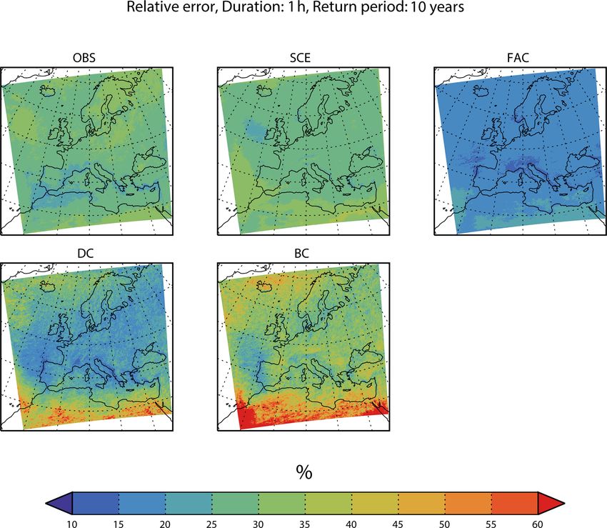
274                    T. Schmith et al.: Identifying robust bias adjustment methods for European extreme precipitation

tracks. Therefore, the statistics of the occurrence of severe     RCMs underestimate hourly extremes and give an erroneous
precipitation events will also most likely change.                spatial distribution.
   Global climate models (GCMs) are the main tools for es-           Extreme convective precipitation of a short duration is thus
timating future climate conditions. A GCM is a global repre-      one of the more challenging phenomena to physically repre-
sentation of the atmosphere, the ocean and the land surface       sent accurately in RCMs. The reason is that convective events
and the interaction between these components. The GCM is          take place on a spatial scale comparable to the RCM grid
then forced with observed greenhouse gas concentrations, at-      spacing of, presently, around 10 km. Therefore, the convec-
mospheric compositions, land use, etc., to represent the past     tive plumes cannot be directly modelled. Instead, the effects
and present climate and with stipulated scenarios of future       of convection are parameterised, i.e. modelled as processes
concentrations of radiative forcing agents to represent the fu-   on larger spatial scales (Arakawa, 2004). Thus, the inability
ture climate.                                                     to reproduce these short-duration extremes can be explained
   Present state-of-the art GCMs from the Coupled Model In-       by the imperfect parameterisation of a sub-grid-scale convec-
tercomparison Project Phase 5 (CMIP5; Taylor et al., 2012)        tion (Prein et al., 2015), which generally leads to a too early
and the recent Coupled Model Intercomparison Project Phase        onset of convective rainfall in the diurnal cycle and the sub-
6 (CMIP6; Eyring et al., 2016) typically have a grid spacing      sequent dampening of the build-up of convective available
of around 100 km or even more. This resolution is too coarse      potential energy (Trenberth et al., 2003).
to describe the effect of regional and local features, such          Thus, even RCMs with their small grid spacing may ex-
as mountains, coastlines and lakes, and to adequately de-         hibit systematic biases for variables related to convective pre-
scribe convective precipitation systems (Eggert et al., 2015).    cipitation. If there is a substantial bias, we should consider
To model the processes on smaller spatial scales, dynamical       adjusting for this in a statistical sense before conducting any
downscaling is applied. Here, the atmospheric and surface         further data analysis. Such adjustment techniques are thor-
fields from a GCM simulation are used as boundary con-            oughly discussed, including requirements and limitations, in
ditions for a regional climate model (RCM) over a smaller         Maraun (2016) and Maraun et al. (2017). There are basi-
region, with a much finer grid spacing, which is typically        cally two main adjustment approaches. In the delta change
around 10 km or even less at present.                             approach, a transformation is established from the present
   An alternative to dynamical downscaling is statistical         to the future climate in the model run. This transformation is
downscaling. Here, large-scale circulation patterns (e.g. the     then applied to the observations to obtain the projected future
North Atlantic Oscillation) are related to small-scale vari-      climate. In the bias correction approach, a transformation is
ables, such as precipitation mean at a station. One assumes       established from present model climate data to the observed
that the large-scale circulation pattern is modelled well by      climate, and this transformation is then applied to the future
the GCM, and therefore, the approach is called perfect prog-      model climate to obtain the projected future climate.
nosis. Using the relationship with the small-scale variables         Both adjustment approaches come in several varieties. In
calibrated on observations, one can obtain modelled local-        the simplest one, the transformation consists of an adjust-
scale variables (present-day and future) from the modelled        ment of the mean, in the case of precipitation, by multiplying
large-scale patterns. A recent overview of these methods and      the mean by a factor. In the more elaborate flavour, the trans-
validation of them can be found in Gutiérrez et al. (2019).       formation is defined by quantile mapping, which also pre-
   The ability of present-day RCMs to reproduce ob-               serves the higher moments. Quantile mapping can use either
served extreme precipitation statistics on daily and sub-daily    empirical quantiles or analytical distribution functions. The
timescales is essential and has been of concern. Earlier stud-    ability of quantile mapping to reduce bias has been demon-
ies analysing this topic have mostly focused on a particular      strated for daily precipitation in the present-day climate by
country, probably due to the lack of sub-daily observational      using observations which are split into calibration and vali-
data covering larger regions, such as, for example, Europe.       dation samples (Piani et al., 2010; Themeßl et al., 2011).
Thus, Hanel and Buishand (2010), Kendon et al. (2014), Ols-          Bias adjustment techniques originate in the field of
son et al. (2015) and Sunyer et al. (2017) studied daily and      weather and ocean forecast modelling, where they are known
hourly extreme precipitation in different European countries      as model output statistics (MOSs). Here, output from a fore-
and reached similar conclusions. First, that the bias of ex-      cast model is adjusted for model deficiencies and local fea-
treme statistics decreases with a smaller grid spacing of the     tures not explicitly resolved by the model. Applying similar
model, and second, that extreme statistics for a 24 h dura-       adjustment techniques to climate model simulations, how-
tion are satisfactorily simulated with a grid spacing of 10 km,   ever, has a complication not present in forecast applications.
while 1 h extreme statistics exhibit substantial biases even at   Climate models are set up and tuned to present-day condi-
this resolution. Recently, Berg et al. (2019) evaluated high-     tions and verified against observations but are then applied
resolution RCMs from the EURO-CORDEX ensemble (Ja-                to future, changed conditions without any possibility of di-
cob et al., 2014) also used here and reached similar conclu-      rectly verifying the model’s performance under these condi-
sions for several countries across Europe. They found that        tions. Therefore, showing that bias adjustment works for the

Hydrol. Earth Syst. Sci., 25, 273–290, 2021                                         https://doi.org/10.5194/hess-25-273-2021
T. Schmith et al.: Identifying robust bias adjustment methods for European extreme precipitation                                275

present-day climate is a necessary but insufficient condition       the real climate system. Thus, one member of the ensemble
for the adjustment to work in the changed climate.                  alternatively plays the role of the pseudo-observation against
   A central concept of adjustment methods is the assumption        which the remaining adjusted models are validated. Thus,
of the stationarity of the bias. For bias correction, this means    the trick is that we know both present and future pseudo-
that the transformation from model to observations is un-           observations.
changed from the present-day climate to the future climate,            The advantage of inter-model cross-validation is that the
while, for delta change, the transformation from the present-       adjustment methods are calibrated under present-day condi-
day climate to future climate is unchanged from model to ob-        tions and validated under future climatic conditions. There-
servation. In the ideal case of stationarity being fulfilled, the   fore, it embraces modelled physical changes between present
adjustment methods will work perfectly and produce perfect          and future climate as, for instance, a shift in the ratio be-
future projections. If stationarity is not fulfilled, adjustments   tween stratiform and convective precipitation. In this respect,
may improve projections or, in the worst cases, may degrade         it is a more realistic setting than validation based on split-
projections, compared to using raw model output. We also            sample test. Also, model and pseudo-observations have the
note that the adjustment methods themselves may influence           same spatial scale, thus avoiding comparing pointwise obser-
the climate change signal of the model, depending on the bias       vations with area-averaged model data as is done in the split-
and the method used (Berg et al., 2012; Haerter et al., 2011;       sample testing. On the other hand, the method assumes that
Themeßl et al., 2012).                                              the modelled present-day is not too different from observa-
   Stationarity has been debated in recent years in the litera-     tions. If this is violated, the method will give error estimates
ture (e.g. Boberg and Christensen, 2012; Buser et al., 2010).       that are too optimistic compared to what can be expected in
Kerkhoff et al. (2014) review and discuss the following two         the real World. Please also see the discussion in Sect. 5.2.
hypotheses: (1) constant bias, which is unchanged between              Inter-model cross-validation has been applied on daily pre-
the present-day and future (i.e. stationarity), and (2) constant    cipitation to evaluate different adjustment methods (Räty
relation, where the bias varies linearly with the signal. Van       et al., 2014). Here, we apply a similar methodology,
Schaeybroeck and Vannitsem (2016) used a pseudo-reality             Europe-wide, to extreme precipitation on hourly and daily
setting with a simplified model and found large changes in          timescales. This has been made possible with the advent of
the bias between the present-day and future for many vari-          the EURO-CORDEX, a large ensemble of high-resolution
ables and a violation of both constant bias and constant re-        RCM simulations with precipitation at an hourly time res-
lation hypothesis. Chen et al. (2015) concluded that precip-        olution. Being more specific, we apply the standard extreme
itation bias is clearly non-stationary over North America in        value analysis to the ensemble of model data for present-day
that variations in bias are comparable to the climate change        and end-21st-century conditions to estimate return levels for
signal. Velázquez et al. (2015) used a pseudo-reality setting       daily and hourly duration. Then, we will apply inter-model
involving two models and concluded that the constancy of            cross-validation on these return levels in order to address the
bias was violated for both precipitation and temperature on         following questions:
monthly timescales. Hui et al. (2019) used a pseudo-reality
setting with GCMs and found a significant non-stationarity           1. Do adjusted return levels perform better, according to
of bias for annual and seasonal temperatures. Besides, they             the inter-model cross-validation, than using raw model
point to a large effect on non-stationarity from internal vari-         data from scenario simulations?
ability.                                                             2. Is there any difference in performance between different
   To thoroughly validate adjustment methods, both a cali-              adjustment methods?
bration data set and an independent data set for validation
are needed. There are two different approaches to obtain this.       3. Are there systematic differences between point 1 and 2,
In split-sample testing, the observations are divided into cal-         depending on the daily and hourly duration?
ibration and validation parts, often in the form of a cross-
validation (e.g. Gudmundsson et al., 2012; Li et al., 2017a, b;      4. Are there regional differences across Europe in the per-
Refsgaard et al., 2014; Themeßl et al., 2011). One variant is           formance of the different adjustment methods?
differential split-sample testing (Klemeš, 1986), where the            Giving qualified answers to these questions can serve as
split in calibration and validation parts is based on clima-        important guidelines for analysis procedures for obtaining
tological factors, such as wet and dry years, encompassing          future extreme precipitation characteristics.
climate changes and variations into the validation.                    The rest of the paper contains a description of the EURO-
   An alternative approach, which we use here, is inter-model       CORDEX data (Sect. 2) and a description of the methods
cross-validation as pursued by Maraun (2012), Räisänen and          used (Sect. 3). Then follow the results (Sect. 4), a discussion
Räty (2013) and Räty et al. (2014), among others. The ratio-        of these (Sect. 5) and, finally, the conclusions (Sect. 6).
nale here is that the members of a multi-model ensemble of
simulations represent different descriptions of the physics of
the climate system, with each of them being not too far from

https://doi.org/10.5194/hess-25-273-2021                                            Hydrol. Earth Syst. Sci., 25, 273–290, 2021
276                   T. Schmith et al.: Identifying robust bias adjustment methods for European extreme precipitation

Table 1. Overview of the 19 EURO-CORDEX GCM–RCM combinations used. The rows show the GCMs while the columns show the RCMs.
The full names of the RCMs are SMHI-RCA4, CLMcom-CCLM4-8-17, KNMI-RACMO22E, DMI-HIRHAM5, MPI-CSC-REMO2009
and CLMcom-ETH-COSMO-crCLIM-v1-1. Each GCM–RCM combination used is represented by a number (1, 3 or 12) indicating which
realisation of the GCM is used for the particular simulation.

                  GCM                                                         RCM
                                                   RCA     CCLM     RACMO       HIRHAM       REMO       COSMO
                  ICHEC-EC-EARTH                     r12               r1           r3
                  MOHC-HadGEM2-ES                     r1               r1           r1
                  CNRM-CERFACS-CNRM-CM5               r1                            r1
                  MPI-M-MPI-ESM-LR                    r1     r2                     r1          r1         r1
                  IPSL-IPSL-CM5A-MR                   r1
                  NCC-NorESM1-M                       r1                            r1                     r1
                  CCCma-CanESM2                              r1
                  MIROC-MIROC5                               r1

2   EURO-CORDEX data

The model simulations used here have been performed
within the framework of EURO-CORDEX (Jacob et al.,
2014; http://euro-cordex.net, last access: January 2021),
which is an international effort aimed at providing RCM cli-
mate simulations for a specific European region (see Fig. 1)
in two standard resolutions with a grid spacing of 0.44◦
(EUR-44; ∼ 50 km) and 0.11◦ (EUR-11; ∼ 12.5 km), respec-
tively. All GCM simulations driving the RCMs follow the
CMIP5 protocol (Taylor et al., 2012) and are forced with his-
torical forcing for the years 1850–2005, followed by the rep-
resentative concentration pathway (RCP) 8.5 scenario for the
years 2006–2100 (until 2099 only for HadGEM-ES).
   We analyse precipitation data in hourly time resolu-
tions from 19 different GCM–RCM combinations from the
EUR-11 simulations shown in Table 1, and we analyse
two 25-year-long time slices from each of these simula-
tions, namely a present-day (years 1981–2005) and end-21st-
century (years 2075–2099) time slice.
   All GCM–RCM combinations we use are represented by
                                                                  Figure 1. Map showing the EURO-CORDEX region (outer frame)
one realisation only, and therefore, the data material used
                                                                  with elevation in colours. PRUDENCE subregions (Christensen and
represents 19 different possible realisations of climate model    Christensen, 2007) used in the analysis are also shown. Note: BI –
physics, though we acknowledge that some GCMs/RCMs                British Isles; IP – Iberian Peninsula; FR – France, ME – mid-
might originate from the same or similar model codes              Europe; SC – Scandinavia; AL – Alps; MD – Mediterranean; EA –
and, therefore, may not be fully independent. The EURO-           Eastern Europe. Red cross marks the point used in Fig. 4.
CORDEX ensemble includes a few simulations which do not
use the standard EUR-11 grid. These were not included in the
analysis since they should have been re-gridded to the EUR-       index that can be generally applied. Any discrimination of
11 grid, which would dampen extreme events, thus introduc-        GCMs depends on area, season and the meteorological field
ing an unnecessary error source.                                  and property being investigated (Gleckler et al., 2008; e.g.
   Generally, GCM results are quite comparable to reality,        their Fig. 9). Furthermore, these tests and selection proce-
and many validation studies of GCMs exist that also keep an       dures are based on subjective criteria and come with major
eye on Europe (e.g. McSweeney et al., 2015). We are aware         caveats that impact the uncertainty range largely (Madsen
of the use in some papers of procedures for selecting how to      et al., 2017). We therefore choose, in accordance with most
choose subsets of available GCMs (e.g. McSweeney et al.,          other similar studies, to use an ensemble of opportunity for
2015; Rowell, 2019). There is, however, no simple quality         the present study.

Hydrol. Earth Syst. Sci., 25, 273–290, 2021                                          https://doi.org/10.5194/hess-25-273-2021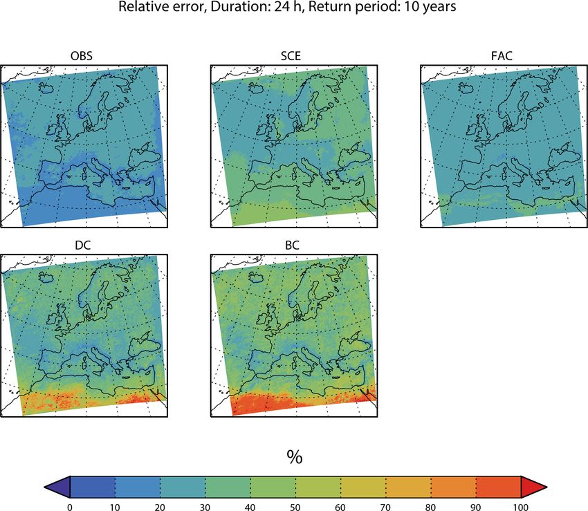
T. Schmith et al.: Identifying robust bias adjustment methods for European extreme precipitation                              277

3     Methods                                                       If we now consider an arbitrary level x with x > x0 , the
                                                                  average number of exceedances per year of x will be the fol-
3.1    Duration                                                   lowing:
Extreme precipitation statistics are often described as a         λx = λ0 [1 − G(x − x0 )] .                                   (1)
function of the timescale involved as intensity–duration–
                                                                  The T year return level, xT , is defined as the precipitation
frequency or depth–duration–frequency curves (e.g.
                                                                  intensity, which is exceeded on average once every T years,
Overeem et al., 2008). We consider two timescales or
                                                                  as follows:
durations. One is a duration of 1 h, which is simply the time
series of hourly precipitation sums available in each RCM         λxT T = 1,
grid point. The other is a duration of 24 h, where a 24 h sum
                                                                  and by combining with Eq. (1) we obtain an expression for
is calculated in a sliding window with a 1 h time step. We
                                                                  the return level, xT , as follows:
will refer to these as hourly and daily duration, respectively.
Our daily duration corresponds to the traditional climato-        λ0 [1 − G(xT − x0 )] T = 1,
logical practice of reporting daily sums but allows heavy
precipitation events to occur over 2 consecutive days. We         from which we calculate the following:
also emphasise that the duration, as defined here, is not the

                                                                         −1       1
actual length of the precipitation events in the model data       xT = G      1−        + x0 .                                 (2)
                                                                                 λ0 T
but merely a concept for defining timescales.
                                                                  Data points to be included in the POT analysis can be se-
3.2    Extreme value analysis                                     lected in two different ways. Either the threshold x0 is spec-
                                                                  ified and λ0 is then a parameter to be determined or, alterna-
Extreme value analysis (EVA) provides methodologies to es-        tively, λ0 is specified and x0 is determined as a parameter. We
timate high quantiles of a statistical distribution from obser-   choose the latter approach, since it is most convenient when
vations. The theory relies on the fundamental convergence         working with data from many different model simulations.
properties of the time series of extreme events; for details,        Choosing λ0 is a point to consider. Too high a value would
we refer to Coles (2001).                                         include too few data points in the estimation, and too low
   There are two main methodologies in EVA for obtaining          a value implies the risk that the exceedances xT − x0 can-
estimates of the high percentiles and the corresponding re-       not be considered as being distributed according to GPD. We
turn levels. In the classical or block maxima method, a gen-      choose λ0 = 3 in accordance with Berg et al. (2019), which
eralised extreme value distribution is fitted to the series of    gives 75 data points for an estimation of the 25-year-long
maxima over a time block, which is usually 1 year. Alterna-       time slices. Hosking and Wallis (1987) investigated the es-
tively, in the peak-over-threshold (POT) or partial-duration      timation of parameters of the GPD and, based on this, warn
series method, which is used here, all peaks with maximum         against using the often-applied maximum likelihood estima-
above a (high) threshold, x0 , are considered. The peaks are      tion for a sample size below 500. Instead, they recommend
assumed to occur independently at an average rate per year        probability-weighted moments, and we have followed this
of λ0 . To ensure independence between peaks, a minimum           advice here.
time separation between peaks is specified. Theory tells us          We required a minimum of a 3 and 24 h separation be-
that, when the threshold goes to infinity, the distribution of    tween peaks for a 1 and 24 h duration, respectively. This is in
the exceedances above the threshold, x − x0 , converges to a      accordance with Berg et al. (2019), and furthermore, synop-
generalised Pareto distribution for which the cumulative dis-     tic experience tells us that this will ensure that neighbouring
tribution function is as follows:                                 peaks are from independent weather systems. We found only
                               1                                 a weak influence of these choices on the results of our anal-
                        x − x0 − ξ

                                                                  ysis.
G (x − x0 ) = 1 − 1 + ξ            , x > x0 .
                          σ                                          In practical applications of EVA, the parameters are esti-
                                                                  mated with large uncertainties due to the limited length of
The parameter σ is the scale and a measure of the width of        the time series. The threshold has the smallest relative uncer-
the distribution. The parameter ξ is the shape and describes      tainty, the scale has a larger relative uncertainty and the shape
the character of the upper tail of the generalised Pareto dis-    has the largest relative uncertainty. Therefore, the relative un-
tribution (GPD); ξ > 0 implies a heavy tail, which usually        certainty of the return levels also increase with increasing T ,
is the case for extreme precipitation events, while ξ < 0 im-     as can be seen from Eq. (2).
plies a thin tail. Note that, quite confusingly, an alternative
sign convention of ξ occurs in the literature (e.g. Hosking       3.3   Bias adjustments and extreme value analysis
and Wallis, 1987).
                                                                  The delta change and bias correction approaches were in-
                                                                  troduced in general terms in Sect. 1. Now we will formulate

https://doi.org/10.5194/hess-25-273-2021                                          Hydrol. Earth Syst. Sci., 25, 273–290, 2021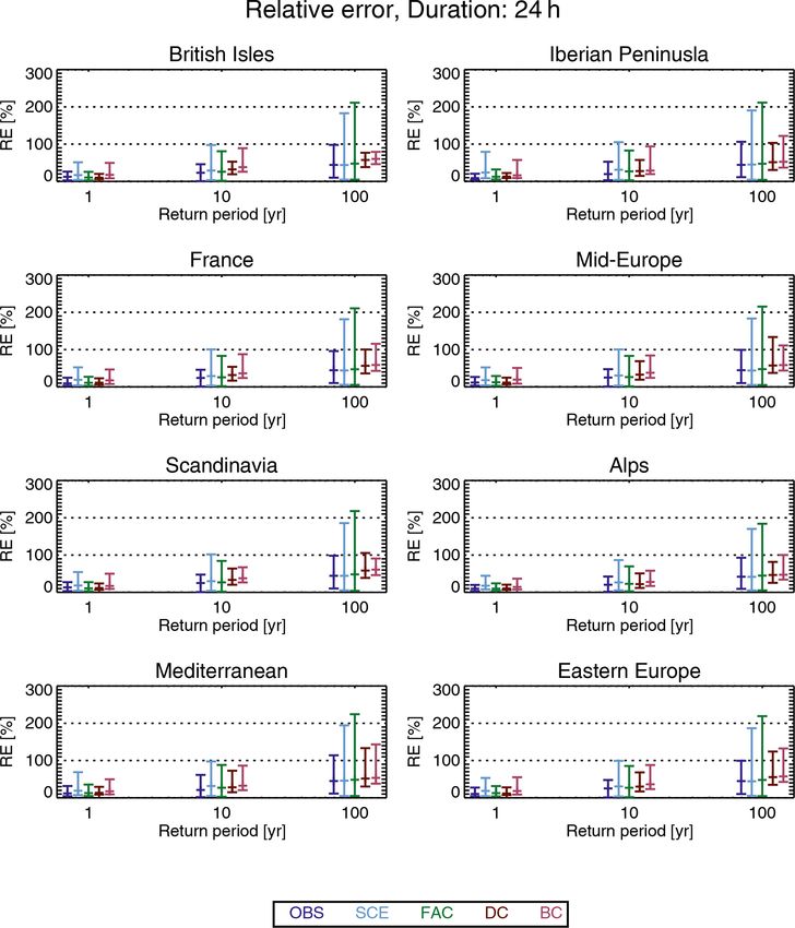
278                    T. Schmith et al.: Identifying robust bias adjustment methods for European extreme precipitation

EVA-based analytical quantile mapping based versions of the        Table 2. Overview of methods used in the inter-comparison.
two approaches. In what follows, OT is the T year return
level estimated from present-day pseudo-observations, while                OBS   (Pseudo-) observations (reference method)
CT (control) and ST (scenario) denote the corresponding re-                SCE   Raw RCM scenario (reference method)
turn levels, estimated from present-day and end-21st-century               FAC   Climate factor on return levels
model data, respectively. Finally, PT (projection) denotes the             DC    Quantile-mapped delta change based on EVA
end-21st-century return level after a bias adjustment has been             BC    Quantile-mapped bias correction based on EVA
applied.

3.3.1   Climate factor on the return levels (FAC)                  where GC and GS are the GPD cumulative distribution func-
                                                                   tions for the data modelled on the present-day (control) and
The simplest adjustment approach is to assume a climate fac-       end-21st-century (scenario), respectively, and C0 and S0 are
tor on the return level (FAC) as follows:                          the corresponding threshold values.
                                                                      For the bias correction (BC) approach, the present-day
PT =       ST /CT      · OT =    OT /CT       · ST .               (control) and pseudo-observed GPD cumulative distribution
           | {z }                | {z }
        Delta change          Bias correction                      functions are quantile mapped to obtain the model bias,
                                                                   which is then applied, using Eq. (3), to the modelled return
        climate factor        climate factor
                                                                   levels for end-21st-century (scenario).
We note that the delta change and bias correction approach         PT = O0 + G−1
are identical for the FAC method.                                             O (GC (ST − C0 )) ,

                                                                   where GO is the GPD cumulative distribution function for
3.3.2   Analytical quantile mapping based on EVA                   the observations and O0 the corresponding threshold.
In the EVA-based quantile mapping, two POT-based extreme           3.3.3    Reference adjustment methods
value distributions with different parameters are matched.
Being more specific, we want to construct a transformation         The performance of the bias adjustment methods described
from x → y defined by the requirement that exceedance rates        above will be compared with the performance of two ref-
above x and y, respectively, are equal for any x as follows:       erence adjustment methods, which are defined below. This
                                                                   is similar to what is practised when verifying predictions,
λx = λy .                                                          where the performance of the prediction should be superior
                                                                   to the performance of reference predictions such as persis-
This implies, according to Eq. (1), that in the following:         tence or climatology.
                                                                    We choose two reference methods. One reference is to
λ0x [1 − Gx (x − x0 )] = λ0y 1 − Gy (y − y0 ) ,
                                                                   simply use, for a given model, the return level calculated
                                                                   from (pseudo-) observations as the projected return level
where Gx is the GPD distribution of the exceedances, x − x0
                                                                   (OBS) as follows:
and λ0x are the associated exceedance rate, and Gy and λ0y
are the similar entities for y.                                    PT = OT .
   To simplify, we let λ0x = λ0y (see Sect. 3.2) and, therefore,
obtain the following:                                              Another reference is to use the raw scenario model output
                                                                   data without any adjustment (SCE) as follows:
Gx (x − x0 ) = Gy (y − y0 ) ,
                                                                   P T = ST .
from which we obtain the following transformation:
                                                                   For an overview of the methods, see Table 2.
y = y0 + G−1
          y (Gx (x − x0 )) .                                 (3)
                                                                   3.4     The inter-model cross-validation procedure in
For the delta change (DC) approach, the modelled GPD dis-                  detail
tribution functions for present-day and end-21st-century con-
ditions are quantile mapped, and the transformation obtained       The inter-model cross-validation goes in detail as follows.
this way is then applied to return levels determined from          Each of the N models are successively regarded as be-
present-day pseudo-observations OT . Thus, the correspond-         ing pseudo-observations. The individual adjustment meth-
ing projected T year return level is the following, according      ods are calibrated on the present-day parts of the pseudo-
to Eq. (3):                                                        observations and model return levels (present-day and end-
                                                                   21st-century) as appropriate, depending on whether it is a
PT = S0 + G−1
           S (GC (OT − C0 )) ,                                     bias correction or delta change method. The calibration is

Hydrol. Earth Syst. Sci., 25, 273–290, 2021                                           https://doi.org/10.5194/hess-25-273-2021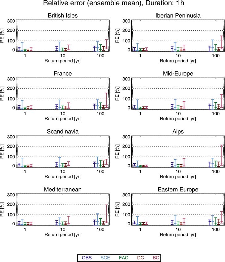
T. Schmith et al.: Identifying robust bias adjustment methods for European extreme precipitation 279
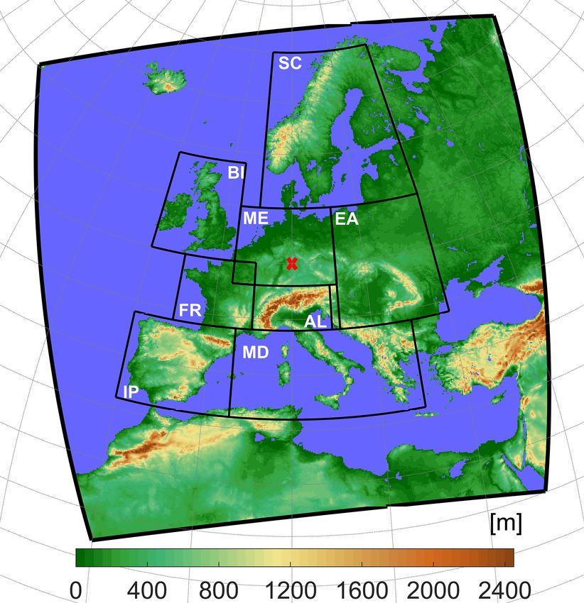
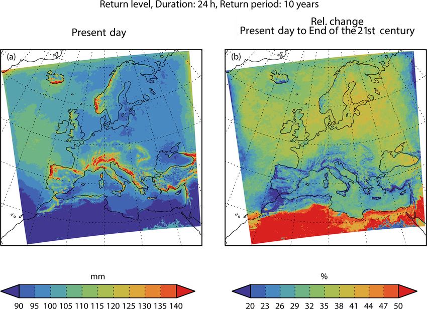
done as described above. The adjustment methods are then We also show, in Fig. 3, the median 10-year return level
applied to present-day observations and model data, again as for a 24 h duration. Again, the largest return levels are found
appropriate, to obtain the adjusted return levels for end-21st- in southern Europe and northwest of the Iberian Peninsula.
century. These are then validated against the return levels for Also, the mountainous regions stand out with higher return
end-21st-century derived from pseudo-observations. levels that are even more pronounced than for a 1 h dura-
The basic validation metric will be the relative error of the tion. The return levels generally increase conditions from the
return levels for end-21st-century for a given duration and present-day to end-21st-century by around the same percent-
return period T , as follows: age as for a 1 h duration, and they are also geographically
homogeneous.
RE = |PT − VT | /VT . To obtain a more detailed impression of the data, Fig. 4
shows the return levels and their changes from the present-
Thus, this determines the absolute difference between the day to end-21st-century for a grid point in northern Germany
projected return level PT obtained from using an adjustment for all 19 model simulations. For a 1 h duration (Fig. 4a), re-
and the validation return level VT estimated from pseudo- turn values increase from the present-day to end-21st-century
observations for end-21st-century divided by the validation in all cases. For a 24 h duration (Fig. 4b), the return levels
return level. This metric is calculated for every grid point typically increase from the present-day to end-21st-century
and for every combination of model or pseudo-observations. but with some exceptions. This behaviour is common to all
Since we have N = 19 model simulations in the ensemble, regions. For both durations, we also note the large spread in
we have N × (N − 1) = 342 different combinations for vali- return levels within the ensemble. The spread is much higher
dating each adjustment method and can make statistics of the than the change between the present and future for most mod-
relative error. This quantifies the average performance of the els; in other words, there is a poor signal-to-noise ratio. This
different methods. is probably a combined effect of different climate signals in
End-user scenarios are often constructed as the median different models and natural variability (Aalbers et al., 2018).
or mean from ensembles. We also tested this in the inter-
model cross-validation set-up. The calibration is performed, 4.2 Inter-model cross-validation
as before, on each of the remaining models and adjusted re-
turn levels for end-21st-century are calculated. But then the In the following, we will present results using two differ-
median of these adjusted future return levels is calculated, ent types of displays. First, we will use spatial maps of the
and this is validated against the future pseudo-observations. median relative error, calculated from all combinations of
Note that this gives only N = 19 different combinations and, model/pseudo-observations. Second, we will, for each ad-
therefore, less robust statistics compared to the above. justment method and for each combination of model/pseudo-
observations, calculate the median relative error over each of
the eight PRUDENCE subregions defined in Christensen and
4 Results Christensen (2007) and shown in Fig. 1. For each region, we
will illustrate the distribution of the relative error across all
4.1 Modelled return levels for conditions in the
combinations of model/pseudo-observations by showing the
present-day and end-21st-century
median and the 5th and 95th percentiles of this distribution.
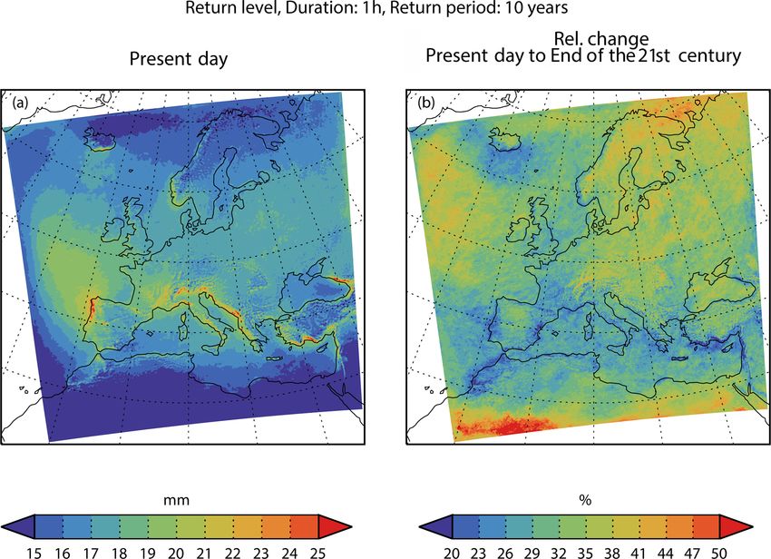
Figure 2 displays the geographical distribution of the 10-year
4.2.1 Results for a 1 h duration
return level for precipitation intensity of a 1 h duration, cal-
culated as the median return level over all 19 model simula- Figure 5 shows the median, across all model/pseudo-
tions. The smallest return levels are mainly found in the arid observation combinations, the relative error for all five meth-
North African region and, to some extent, in the Norwegian ods for 1 h duration and the 10-year return period.
Sea, while the largest return levels are found in southern Eu- First, we look at the reference methods. Relative errors
rope and in the Atlantic northwest of the Iberian Peninsula. from the OBS method are in the range of 20 %–40 %. The
Mountainous regions, such as the Alps and western Norway, lowest values are found in the Mediterranean, western France
stand out as having higher return levels than their surround- and the Atlantic west of the Mediterranean; the highest val-
ings. This supports the idea that the models are not totally ues are in the Atlantic west of Ireland and in Scandinavia.
unrealistic in modelling extreme precipitation. The SCE method has errors in the interval of 25 %–45 %,
There is a general increase in the range of 20 %–40 % in with the lowest values in the Atlantic west of Ireland; the
climatic conditions from the present-day to end-21st-century. largest values are over parts of the Atlantic and northern
The relative changes are geographically quite uniform across Africa. The two reference methods give rather similar results,
the area. For instance, no evident difference between the land but the OBS method slightly outperforms SCE in the south,
and sea appears. Moreover, the mountainous regions do not while the opposite is true in the north.
stand out from their surroundings.
https://doi.org/10.5194/hess-25-273-2021 Hydrol. Earth Syst. Sci., 25, 273–290, 2021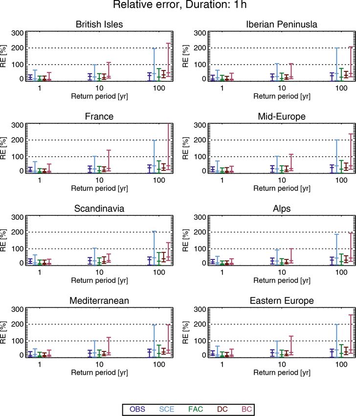
280                      T. Schmith et al.: Identifying robust bias adjustment methods for European extreme precipitation

Figure 2. Geographical distribution of the 10-year return level of precipitation intensity for 1 h duration for the present-day (a) and relative
change from the present-day to end-21st-century (b). In each grid point, values are the median return level over all 19 model simulations.

Figure 3. As in Fig. 2 but for a 24 h duration.

   The relative error of FAC is below 20 % in most places.                Africa) that of FAC. That said, the concept of relative error
Everywhere it is smaller than the relative error of the ref-              should be used with care in an arid region, such as north-
erence methods OBS and SCE. The DC method has a rela-                     ern Africa. But, from this result, it is not justifiable to use
tive error comparable to (e.g. western France, western Iberia             the more complicated DC in favour of the simpler FAC. Fi-
and eastern Atlantic) or larger than (in particular, northern             nally, the relative error of BC is above both DC and FAC ev-

Hydrol. Earth Syst. Sci., 25, 273–290, 2021                                                   https://doi.org/10.5194/hess-25-273-2021
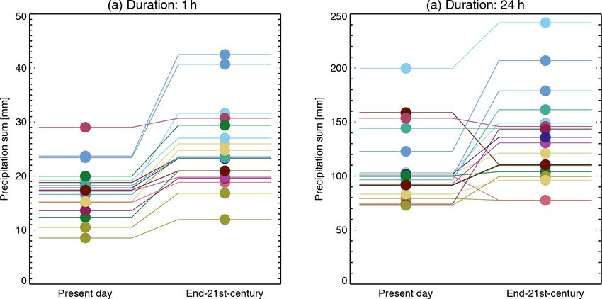
T. Schmith et al.: Identifying robust bias adjustment methods for European extreme precipitation                                      281

Figure 4. Modelled return levels at 50◦ N, 10◦ E (northern Germany; marked with a red cross in Fig. 1) for the present and future for a
10-year return period and 1 and 24 h durations. Different colours represent the 19 different GCM–RCM simulations listed in Table 1.

Figure 5. Geographical distribution of the relative error of the end-21st-century 10-year return level for a 1 h duration precipitation in-
tensity from the inter-model cross-validation. Colours show the median of the relative error calculated over all model/pseudo-observation
combinations. Panels show the different adjustment methods.

https://doi.org/10.5194/hess-25-273-2021                                                 Hydrol. Earth Syst. Sci., 25, 273–290, 2021
282                    T. Schmith et al.: Identifying robust bias adjustment methods for European extreme precipitation

erywhere, indicating the poorest performance of all methods         characteristics hold for FAC. The quantile-mapping methods
considered.                                                         DC and BC have slightly larger median values, but the 95th
   The statistical distribution of the relative error is shown      percentile is smaller than for FAC. All these characteristics
in Fig. 6 for the eight PRUDENCE subregions (see Fig. 1).           hold for all subregions.
We first note that the distribution of relative error is shifted
towards higher values for larger return periods, as expected.       4.2.3    Ensemble median
Next, we note that the two reference methods, OBS and SCE,
behave differently. SCE generally has a slightly larger me-         Inter-model cross-validation of pseudo-observations against
dian relative error, but the 95th percentile is much larger for     the model ensemble median, as described in Sect. 3.4, was
SCE than for OBS, in particular for large return periods.           also carried out. For a 1 h duration, the distribution of the rel-
Thus, OBS performs better overall than SCE, meaning that            ative error is shown in Fig. 9. By comparing this with Fig. 6,
using present-day pseudo-observations to estimate the pro-          the distribution of the relative error does not change much
jected return levels for end-21st-century yields a better rela-     overall. However, for many of the subregions considered, and
tive error than using raw modelled scenario data.                   for the longer return periods, FAC and BC have a smaller
   The FAC method generally has the best overall perfor-            95th percentile for cross-validation against model ensemble
mance, both in terms of the median and the 95th percentile          means than against individual models.
of the relative error. The DC method has a slightly poorer             In addition, the distribution of the relative errors does not
performance than FAC, both in terms of the median and the           change much for a 24 h duration when shifting to a validation
95th percentile of the relative error. Finally, BC has a poorer     against the ensemble median (not shown).
performance than DC, when comparing the median of the
                                                                    4.3     Further analysis on conditions for skill
relative error and, in particular, the 95th percentile.
   In summary, for a 1 h duration, the method with the best         To obtain further insight into the difference in performance
performance is using a climate factor on the return levels          between hourly and daily precipitation, we consider, for a
(FAC). This method outperforms both reference methods and           given return period, the relationship between the bias factor
the more sophisticated methods based on quantile mapping,           for present-day BP ,T = O  CT
                                                                                                   and BF,T = VSTT end-21st-century
                                                                                                 T
i.e. DC and BC, with the latter having the poorest overall per-     for all model/pseudo-observation combinations (see Fig. 10).
formance of them all. Note that DC is comparing GPDs from              In this figure, the relationship between bias factors in the
the same model, whereas BC is comparing GPDs from dif-              present-day and end-21st-century appears more pronounced
ferent models. If the difference, in terms of GPD parameters,       for 1 h duration than for 24 h duration. That said, it must be
between two models in the present-day climate is typically          borne in mind that if the point (x, y) is in the plot, then so
larger than the difference between the same model for the cli-      is the point (1/y, 1/x), and this implies an inherent tendency
mate in the present-day and end-21st-century, it can explain        towards a fan-like spread of points from (0, 0), as seen on
the different results.                                              both plots.
                                                                       To quantify the strength of the above relationship, we de-
4.2.2   Results for a 24 h duration                                 fine an index as follows:

For a 24 h duration (see Fig. 7), OBS has the lowest median                  |BF − BP |
                                                                    R=                       ,
relative error (less than 30 %) in most regions of all the ad-              (BF + BP ) /2
justment methods, while SCE has higher relative error in the
interval of approximately 30 %–60 %, with the highest val-          where h·i means averaging over combinations of
ues in North Africa. FAC has relative errors in between those       model/pseudo-observations. This index is an extension
of OBS and SCE. Of the quantile-mapping methods, DC has             of the index introduced by Maurer et al. (2013). It is the
relative errors in the interval of approximately 20 %–80 %,         ensemble average of the relative absolute difference between
which is larger than FAC in most places, and finally, BC has,       the present-day and future bias. A value of R = 0 means
as for a 1 h duration, the largest median relative errors of all    that these biases are equal, i.e. perfect stationarity, and
the methods.                                                        the smaller the value of R, the closer to stationarity (in an
   As for the 1 h duration, we also compare the entire statis-      ensemble sense).
tical distribution of the relative error of the different adjust-      Values of R are given in the upper left corner of each panel
ment methods for all three return periods (Fig. 8), and again,      of Fig. 10, and they also support the partial relationships de-
both the median and 95th percentile of the relative error in-       scribed above and a stronger one for hourly duration. These
creases for larger return periods, as expected. Furthermore,        relations are important since they could explain the generally
OBS seems, surprisingly, to have a small median relative er-        good performance of the FAC method seen in the previous
ror and the smallest 95th percentile of all methods considered      section. Suppose that BP ,T = BF,T , then, in the following:
for all subregions. SCE has a median not too different from
that of OBS, but the 95th percentile is much larger. Similar

Hydrol. Earth Syst. Sci., 25, 273–290, 2021                                            https://doi.org/10.5194/hess-25-273-2021
T. Schmith et al.: Identifying robust bias adjustment methods for European extreme precipitation 283
Figure 6. Statistical distribution (median and 5th and 95th percentile) of the relative error of the inter-model cross-validation for a 1 h duration
for 1, 10 and 100-year return periods. Panels represent the PRUDENCE subregions shown in Fig. 1. Each colour represents an adjustment
method (see Table 2).
5 Discussion
ST OT VT
PT = OT = ST = ST BP = ST BF = ST = VT ,
CT CT ST
5.1 Relation with other studies
and the FAC method will therefore adjust perfectly.
We also note that daily data, due to the summation, would
The study by Räty et al. (2014) touches upon issues related
have less erratic behaviour than hourly data, and therefore,
to ours. However, our study includes smaller temporal scales
we would expect any relationship to be less masked by noise
(hourly and daily) and higher return periods (up to 100 years
for daily data than for hourly data from purely statistical
vs. the 99.9th percentile of daily precipitation corresponding
grounds. Therefore, any explanation as to why it is opposite
to a return period of around 3 years). Nevertheless, the two
should probably be found in physics or the details of mod-
studies agree in their main conclusion, namely that applying
elling. We will discuss this further in Sect. 5.3.
a bias adjustment seems to offer an additional level of re-
alism to the processed data series, including in the climate
projections, as compared to using unadjusted model results.
The two studies both support the somewhat surprising con-
clusion that using present-day (pseudo-) observations as the
https://doi.org/10.5194/hess-25-273-2021 Hydrol. Earth Syst. Sci., 25, 273–290, 2021284 T. Schmith et al.: Identifying robust bias adjustment methods for European extreme precipitation
Figure 7. As in Fig. 5 but for a 24 h duration.
scenario gives a skill comparable to that of the bias adjust- sented adjustment methods to hourly data from these mod-
ment methods. els. Instead, the present work should be seen as a statisti-
Kallache et al. (2011) proposed a correction method cal exercise, and the methods can, in the future, be applied
for extremes, i.e. cumulative distribution function transfer to convection-permitting model simulations that better rep-
(CDF-t), and obtained good validation result with the calibra- resent the convective process. The results from the present
tion/validation split of historical data from southern France. work would apply equally to that case.
The CDF-t method was applied by Laflamme et al. (2016) With the advent of convective-permitting models, a more
on daily New England data, who concluded that “down- realistic modelling of convective precipitation events is
scaled results are highly dependent on RCM and GCM model within reach, and a change in the characteristics of such
choice”. events is seen (Kendon et al., 2017; Lenderink et al., 2019;
Prein et al., 2015). This next generation of convection-
5.2 Convection in RCMs permitting RCMs with a grid spacing of a few kilometres
allows a much better representation of the diurnal cycle and
The grid spacing of present state-of-the-art RCMs available convective systems as a whole (Prein et al., 2015). With that
in large ensembles, such as CORDEX, is around 10 km, in mind, we foresee redoing the analysis when a suitable en-
and at this resolution, it is necessary to describe convection semble of convective-permitting RCM simulations becomes
through parameterisations. This is obviously an important available.
deficit for our purpose, since this could represent a system-
atic bias in all our simulations and, therefore, violate our un- 5.3 Stationarity of bias
derlying assumptions that the individual model simulations
and the real-world observations behave similarly in a physi- The success of applying bias adjustment to climate model
cal sense. Thus, we do not promote naively applying the pre- simulations is linked to the biases being stationary, i.e.
Hydrol. Earth Syst. Sci., 25, 273–290, 2021 https://doi.org/10.5194/hess-25-273-2021T. Schmith et al.: Identifying robust bias adjustment methods for European extreme precipitation 285
Figure 8. As in Fig. 6 but for a 24 h duration.
present and future biases being more or less identical. In dynamic contribution. In addition to this, there is a dynamic
Sect. 4.3, we showed (in Fig. 10) that this was the case for contribution, and this may explain the differences between
a 1 h duration and less so for a 24 h duration in our pseudo- the hourly and daily relation seen in Fig. 10. The rationale is
reality setting. Such a relationship is an example of an emer- that hourly extremes are entirely due to convective precipita-
gent constraint (Collins et al., 2012). This is a model-based tion events with almost no dynamic contribution (Lenderink
concept, originally introduced to explain that models which et al., 2019), while daily extremes are a mixture of convec-
have too warm (cold) a present-day climate tend to have tive events and large-scale strong precipitation, of which the
a relatively warmer (colder) future climate. The reason for latter has a more significant dynamic contribution (Pfahl et
this is that it is the same underlying physics which gener- al., 2017), causing the less marked emergent constraint for
ates the present-day and future temperatures (Christensen the daily timescale. This interpretation is also supported in
and Boberg, 2012). Fig. 4, in which daily precipitation sees some crossovers (fu-
We suggest that our observed emergent constraints could ture return level smaller than the present), whereas hourly
be explained in a similar manner, namely as a result of precipitation does not have any crossovers.
the Clausius–Clapeyron relation linking atmospheric tem-
perature changes to changes in its humidity content and, 5.4 The spatial scale
thereby, precipitation changes. The change prescribed by the
Clausius–Clapeyron equation is usually termed the thermo- In the definition of model bias, it is tacitly assumed that the
observational data set has the same spatial resolution as the
https://doi.org/10.5194/hess-25-273-2021 Hydrol. Earth Syst. Sci., 25, 273–290, 2021286 T. Schmith et al.: Identifying robust bias adjustment methods for European extreme precipitation
Figure 9. As in Fig. 6 but for the inter-model cross-validation against ensemble medians.
model data. In practice, however, it is rarely possible to sep- ibration to observed conditions (Haerter et al., 2015; Refs-
arate the bias from a spatial-scale mismatch. For instance, if gaard et al., 2014).
we compare modelled precipitation, which represents aver-
ages over a grid box, with rain gauge data, which represent a 5.5 Adjustment methods not included in the study
point, there can be a quite substantial mismatch for extreme
events (Eggert et al., 2015; Haylock et al., 2008). Therefore, Only the basic adjustment methods have been included in
if the bias is adjusted towards such point values, it may lead our study. The simple climate factor approach has been ap-
to further complications (Maraun, 2013). plied in numerous hydrological applications (DeGaetano and
Sometimes, though, it is desirable to include the scale mis- Castellano, 2017; Sunyer et al., 2015 and other sources). We
match in the bias adjustment. Many impact models, e.g. hy- also wanted to test quantile-mapping approaches, which in
drological models, are tuned to perform well with local ob- extreme value theory takes the form of a parametric transfer
servational data as input. This presents an additional chal- function. This we have applied in two flavours in the spirit of
lenge if this impact model is to be driven by climate model Räty et al. (2014). Finally, we wanted to benchmark against
data for climate change studies, since the climate model will the canonical benchmark methods, namely observations and
have biases in its climate characteristics (mean, variability, raw model output.
etc.) compared to those of the observed data. Applying the There is a myriad of more specialised methods which are
adjustment step, the hydrological model can rely on its cal- each tailored to account for a particular deficit of the simpler
methods. First, there is the issue of whether it is, for pre-
Hydrol. Earth Syst. Sci., 25, 273–290, 2021 https://doi.org/10.5194/hess-25-273-2021T. Schmith et al.: Identifying robust bias adjustment methods for European extreme precipitation 287
simulation in turn from the ensemble plays the role of obser-
vations extending into the future. The return levels obtained
from each of the remaining model simulations are then ad-
justed in the present-day period, using different adjustment
methods. Then the same adjustment methods are applied to
the model data for end-21st-century to obtain projected re-
turn levels, which are then compared with the corresponding
pseudo-realistic future return levels.
The main result of this inter-comparison is that, compared
to using the unadjusted model runs, applying bias adjustment
methods improves projected extreme precipitation return lev-
els. Can an overall superior adjustment methodology be ap-
pointed? For an hourly duration, the method to recommend
Figure 10. Relationship between bias factors in the present-day and
end-21st-century in 10-year return levels for the mid-Europe sub-
(with the smallest relative error) is the simple climate factor
region for all model/pseudo-observation combinations. (a) The 1 h approach, FAC, which is better in terms of the relative er-
duration and (b) 24 h duration, respectively. Numbers in upper left ror than the more complicated analytical quantile-mapping
corners are the R indices. See text for details. methods based on EVA, DC and, in particular, BC. For a
daily duration, the OBS method performs surprisingly well,
with the smallest 95th percentile of the relative error. Fur-
cipitation, more reasonable to map relative quantile changes thermore, the quantile-mapping methods perform better than
rather than absolute ones (Cannon et al., 2015). It has also FAC, with DC having the smallest relative error. These con-
been argued that a bias correction method should preserve clusions hold regardless of the subregion considered. We also
long-term trends, i.e. the climate signal, and only adjust the cross-validated against model ensemble means; this gave, in
shorter timescales, as extensively discussed in Cannon et general, similar results without significant changes in the dis-
al. (2015). Then multivariate methods have been argued for tribution of the relative error.
and applied in order to preserve relationships between vari- Finally, we registered emergent constraints between biases
ables (Cannon, 2018) and nested methods to account for dif- in the present-day and end-21st-century. This was more pro-
ferent biases for different timescales (Mehrotra et al., 2018). nounced for hourly than for daily timescales. This could be
Also, methods to correct for systematic displacement of vari- caused by hourly precipitation being more directly linked
able features in complex terrain have been suggested and ap- to the Clausius–Clapeyron response, but this requires more
plied (Maraun and Widmann, 2015). Finally, Li et al. (2018) clarification in future work.
adjust stratiform and convective precipitation separately in-
stead of adjusting the total precipitation. In this way, any fu-
ture change in the ratio between the two types of precipitation Data availability. The hourly EURO-CORDEX precipitation data
is accounted for. are not part of the standard suite of CORDEX and are therefore
It could be interesting to examine the above methods in neither produced nor shared by all modelling groups. The data used
future studies, though we acknowledge it would be a quite in this study may be obtained upon request from each modelling
group. The interactive data language (IDL) code used in the analysis
extensive work. We can, at present, only guess at the out-
can be requested from Torben Schmith.
come of such work, but the more refined methods may not
perform too well in the inter-model cross-validation setting.
The reason for this suspicion is that these methods, while be- Author contributions. TS and PT designed the analysis, with con-
ing more elaborate, in most cases also have more parameters tributions from the other co-authors, and programmed the analysis
to be estimated, implying a higher risk of overfitting. An ar- software. PB, FB, OBC and PT prepared the data. TS prepared the
gument in favour of this is that the present study shows that paper with contributions from PT, PB, FB, OBC, BC, JHC, CS,
the more elaborate quantile-mapping methods of DC or BC and MSM.
do not outperform the simpler FAC method.
Competing interests. The authors declare that they have no conflict
6 Conclusions of interest.
Based on hourly precipitation data from a 19-member en-
semble of climate simulations, we have investigated the ben- Acknowledgements. This work has been supported by the European
efit of bias adjusting extreme precipitation return levels on Commission through the Horizon 2020 Programme for Research
hourly and daily timescales and evaluated the different meth- and Innovation under the EUCP project (grant no. 776613). Part of
the funding was provided by the Danish State through the Danish
ods. This is done in a pseudo-reality setting, where one model
https://doi.org/10.5194/hess-25-273-2021 Hydrol. Earth Syst. Sci., 25, 273–290, 2021288 T. Schmith et al.: Identifying robust bias adjustment methods for European extreme precipitation
Climate Atlas. Peter Berg was funded by the project AQUACLEW, Cannon, A. J.: Multivariate quantile mapping bias correction: an N-
which is part of ERA4CS, an ERA-NET initiated by JPI Climate, dimensional probability density function transform for climate
and is funded by FORMAS (SE), DLR (DE), BMWFW (AT), model simulations of multiple variables, Clim. Dynam., 50, 31–
IFD (DK), MINECO (ES) and ANR (FR), with co-funding by the 49, https://doi.org/10.1007/s00382-017-3580-6, 2018.
European Commission (grant no. 690462). Some of the simulations Cannon, A. J., Sobie, S. R., and Murdock, T. Q.: Bias Correction of
were performed in the Copernicus C3S project C3S_34b (PRINCI- GCM Precipitation by Quantile Mapping: How Well Do Methods
PLES). We acknowledge the World Climate Research Programme’s Preserve Changes in Quantiles and Extremes?, J. Climate, 28,
Working Group on Regional Climate, the Working Group on Cou- 6938–6959, https://doi.org/10.1175/JCLI-D-14-00754.1, 2015.
pled Modelling, and the former coordinating body of CORDEX Chen, J., Brissette, F. P., and Lucas-Picher, P.: Assessing the
and responsible panel for CMIP5. We thank the climate mod- limits of bias-correcting climate model outputs for climate
elling groups (listed in Table 1 of this paper) for producing and change impact studies, J. Geophys. Res.-Atmos., 120, 1123–
making their model output available. We also acknowledge the 1136, https://doi.org/10.1002/2014JD022635, 2015.
Earth System Grid Federation infrastructure, an international ef- Christensen, J. H. and Boberg, F.: Temperature dependent climate
fort led by the US Department of Energy’s Program for Climate projection deficiencies in CMIP5 models, Geophys. Res. Lett.,
Model Diagnosis and Intercomparison, the European Network for 39, 24705, https://doi.org/10.1029/2012GL053650, 2012.
Earth System Modelling and other partners in the Global Organ- Christensen, J. H. and Christensen, O. B.: A summary of the
isation for Earth System Science Portals (GO-ESSP). It is appre- PRUDENCE model projections of changes in European cli-
ciated that Geert Lenderink, KNMI, Claas Teichmann, GERICS, mate by the end of this century, Climatic Change, 81, 7–30,
and Heimo Truhetz, University of Graz, made model data of hourly https://doi.org/10.1007/s10584-006-9210-7, 2007.
precipitation available for analysis. We appreciate the constructive Coles, S.: An introduction to statistical modeling of extreme values,
comments from Jorn van de Velde, from two anonymous refer- Springer, London, UK, 2001.
ees, and from Timo Kelder, Robert Wilby, Tim Marjoribanks and Collins, M., Chandler, R. E., Cox, P. M., Huthnance, J.
Louise Slater. M., Rougier, J., and Stephenson, D. B.: Quantifying fu-
ture climate change, Nat. Clim. Change, 2, 403–409,
https://doi.org/10.1038/nclimate1414, 2012.
Financial support. This research has been supported by the Euro- DeGaetano, A. T. and Castellano, C. M.: Future projections of ex-
pean Commission (grant no. EUCP 776613). treme precipitation intensity-duration-frequency curves for cli-
mate adaptation planning in New York State, Clim. Serv., 5, 23–
35, https://doi.org/10.1016/j.cliser.2017.03.003, 2017.
Review statement. This paper was edited by Nadav Peleg and re- Eggert, B., Berg, P., Haerter, J. O., Jacob, D., and Moseley, C.: Tem-
viewed by Jorn Van de Velde and two anonymous referees. poral and spatial scaling impacts on extreme precipitation, At-
mos. Chem. Phys., 15, 5957–5971, https://doi.org/10.5194/acp-
15-5957-2015, 2015.
Eyring, V., Bony, S., Meehl, G. A., Senior, C. A., Stevens, B.,
Stouffer, R. J., and Taylor, K. E.: Overview of the Coupled
References Model Intercomparison Project Phase 6 (CMIP6) experimen-
tal design and organization, Geosci. Model Dev., 9, 1937–1958,
Aalbers, E. E., Lenderink, G., van Meijgaard, E., and van den Hurk, https://doi.org/10.5194/gmd-9-1937-2016, 2016.
B. J. J. M.: Local-scale changes in mean and heavy precipita- Gleckler, P. J., Taylor, K. E., and Doutriaux, C.: Performance
tion in Western Europe, climate change or internal variability?, metrics for climate models, J. Geophys. Res., 113, D06104,
Clim. Dynam., 50, 4745–4766, https://doi.org/10.1007/s00382- https://doi.org/10.1029/2007JD008972, 2008.
017-3901-9, 2018. Gudmundsson, L., Bremnes, J. B., Haugen, J. E., and Engen-
Arakawa, A.: The Cumulus Parameterization Problem: Past, Skaugen, T.: Technical Note: Downscaling RCM precipitation
Present, and Future, J. Climate, 17, 2493–2525, 2004. to the station scale using statistical transformations – a com-
Berg, P., Feldmann, H., and Panitz, H.-J.: Bias correction of high parison of methods, Hydrol. Earth Syst. Sci., 16, 3383–3390,
resolution regional climate model data, J. Hydrol., 448–449, 80– https://doi.org/10.5194/hess-16-3383-2012, 2012.
92, https://doi.org/10.1016/j.jhydrol.2012.04.026, 2012. Gutiérrez, J. M., Maraun, D., Widmann, M., Huth, R., Hertig, E.,
Berg, P., Christensen, O. B., Klehmet, K., Lenderink, G., Ols- Benestad, R., Roessler, O., Wibig, J., Wilcke, R., Kotlarski, S.,
son, J., Teichmann, C., and Yang, W.: Summertime precipi- San Martín, D., Herrera, S., Bedia, J., Casanueva, A., Man-
tation extremes in a EURO-CORDEX 0.11◦ ensemble at an zanas, R., Iturbide, M., Vrac, M., Dubrovsky, M., Ribalaygua,
hourly resolution, Nat. Hazards Earth Syst. Sci., 19, 957–971, J., Pórtoles, J., Räty, O., Räisänen, J., Hingray, B., Raynaud, D.,
https://doi.org/10.5194/nhess-19-957-2019, 2019. Casado, M. J., Ramos, P., Zerenner, T., Turco, M., Bosshard,
Boberg, F. and Christensen, J. H.: Overestimation of T., Štěpánek, P., Bartholy, J., Pongracz, R., Keller, D. E., Fis-
Mediterranean summer temperature projections due to cher, A. M., Cardoso, R. M., Soares, P. M. M., Czernecki, B.,
model deficiencies, Nat. Clim. Change, 2, 433–436, and Pagé, C.: An intercomparison of a large ensemble of statisti-
https://doi.org/10.1038/NCLIMATE1454, 2012. cal downscaling methods over Europe: Results from the VALUE
Buser, C., Künsch, H., and Schär, C.: Bayesian multi- perfect predictor cross-validation experiment, Int. J. Climatol.,
model projections of climate: generalization and applica- 39, 3750–3785, https://doi.org/10.1002/joc.5462, 2019.
tion to ENSEMBLES results, Clim. Res., 44, 227–241,
https://doi.org/10.3354/cr00895, 2010.
Hydrol. Earth Syst. Sci., 25, 273–290, 2021 https://doi.org/10.5194/hess-25-273-2021You can also read