Near-surface structure of the North Anatolian Fault zone from Rayleigh and Love wave tomography using ambient seismic noise - Solid Earth
←
→
Page content transcription
If your browser does not render page correctly, please read the page content below
Solid Earth, 10, 363–378, 2019
https://doi.org/10.5194/se-10-363-2019
© Author(s) 2019. This work is distributed under
the Creative Commons Attribution 4.0 License.

Near-surface structure of the North Anatolian Fault zone from
Rayleigh and Love wave tomography using ambient seismic noise
George Taylor1,a , Sebastian Rost1 , Gregory A. Houseman1 , and Gregor Hillers2,a
1 School of Earth and Environment, University of Leeds, LS2 9JT Leeds, UK
2 Institutdes Sciences de la Terre, Université Grenoble-Alpes, 38041 Grenoble, France
a now at: Institute of Seismology, University of Helsinki, 00014 Helsinki, Finland

Correspondence: George Taylor (george.taylor@helsinki.fi)

Received: 20 September 2018 – Discussion started: 9 October 2018
Revised: 29 January 2019 – Accepted: 10 February 2019 – Published: 6 March 2019

Abstract. We use observations of surface waves in the am-           1   Introduction
bient noise field recorded at a dense seismic array to im-
age the North Anatolian Fault zone (NAFZ) in the region of
the 1999 magnitude 7.6 Izmit earthquake in western Turkey.          The formation of fault zones appears to be a balance be-
The NAFZ is a major strike-slip fault system extending              tween the accommodation of the tectonic strain field and the
 ∼ 1200 km across northern Turkey that poses a high level           exploitation of pre-existing weak zones such as tectonic su-
of seismic hazard, particularly to the city of Istanbul. We         ture zones or lithological boundaries (e.g. Bercovici and Ri-
obtain maps of phase velocity variation using surface wave          card, 2014; Dayem et al., 2009; Gerbi et al., 2016; Tapponier
tomography applied to Rayleigh and Love waves and con-              et al., 1982). Studying how structural changes affect strain
struct high-resolution images of S-wave velocity in the upper       localization in the upper crust is critical to understanding the
10 km of a 70 × 30 km region around Lake Sapanca. We ob-            earthquake cycle (Bürgmann and Dresen, 2008). Imaging the
serve low S-wave velocities (< 2.5 km s−1 ) associated with         seismic velocity structure of fault zones provides information
the Adapazari and Pamukova sedimentary basins, as well as           essential to understanding the long-term behaviour of faults
the northern branch of the NAFZ. In the Armutlu Block,              and the earthquakes that occur on them.
between the two major branches of the NAFZ, we image                   Here we interpret images from ambient noise surface wave
higher velocities (> 3.2 km s−1 ) associated with a shallow         tomography of the upper 10 km of the North Anatolian Fault
crystalline basement. We measure azimuthal anisotropy in            zone (NAFZ), Turkey, in the rupture zone of the 1999 Izmit
our phase velocity observations, with the fast direction seem-      earthquake. This allows us to study the near-surface structure
ing to align with the strike of the fault at periods shorter than   of a recently ruptured fault. The NAFZ is a ∼ 1200 km long
4 s. At longer periods up to 10 s, the fast direction aligns with   strike-slip fault that forms the boundary between the Ana-
the direction of maximum extension for the region (∼ 45◦ ).         tolian block and the Eurasian continent. Progressively local-
The signatures of both the northern and southern branches           ized since the middle Miocene (∼ 3 Ma), the NAFZ propa-
of the NAFZ are clearly associated with strong gradients in         gated westward from the Karliova Triple Junction in east-
seismic velocity that also denote the boundaries of major tec-      ern Turkey across northern Anatolia and reached the Izmit–
tonic units. Our results support the conclusion that the devel-     Adapazari region ∼ 200 ka, although a more broad zone of
opment of the NAFZ has exploited this pre-existing contrast         shear deformation was present since the middle Miocene
in physical properties.                                             (Sengör et al., 2005). The motion of Anatolia is driven by
                                                                    a gradient of lithospheric gravitational potential energy that
                                                                    extends across the Anatolian Peninsula (England et al., 2016)
                                                                    and is sustained by the collision between the Arabian and
                                                                    Eurasian plate in the east and the roll-back of the Hellenic

Published by Copernicus Publications on behalf of the European Geosciences Union.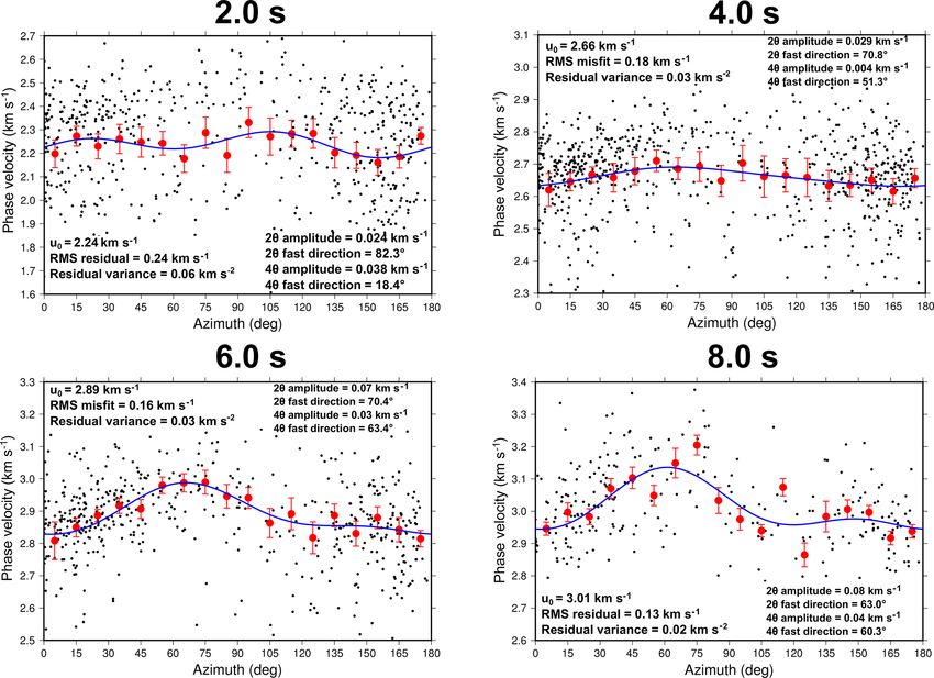
364                                                                         G. Taylor et al.: NAFZ surface wave tomography

trench to the south-west (Flerit et al., 2004; Reilinger et al.,    Sakarya University deployed a temporary array of seismome-
1997). Since 1939 a westward-propagating sequence of large          ters across the rupture zone of the 1999 Izmit earthquake
earthquakes (Mw > 7.0) has occurred along the NAFZ (Stein           between May 2012 and October 2013 (Kahraman et al.,
et al., 1997). The 1999 Izmit (Mw 7.6) and Düzce (Mw 7.2)           2015). The array, known as the Dense Array for Northern
earthquakes are the most recent in this sequence (Barka et al.,     Anatolia, included 62 three-component seismometers in a
2002), and the NAFZ continues to pose a significant seismic         70 km × 35 km rectangular grid (Fig. 1) and an approximate
hazard to the region.                                               station spacing of 7 km. Also included were three stations of
   In the Izmit–Adapazari region, the NAFZ is split into            the KOERI national network located within the main grid of
northern and southern branches (Fig. 1). The northern branch        the DANA array: GULT, SAUV and SPNC. DANA was de-
has seen more seismic activity historically, but microseismic-      ployed over both strands of the NAFZ in this region, with
ity in this region does not appear to be strongly localized to      stations sited on all three of the major crustal units described
the major fault strands (Altuncu Poyraz et al., 2015). The          above (Fig. 1).
northern branch of the fault appears to exploit the so-called          Short-period surface waves from ambient noise have been
Intra-Pontide suture between the Eurasian continent and sed-        used to study the upper crust in the vicinity of active fault
imentary accretionary complexes formed during the closure           zones in the past (e.g. Lin et al., 2013; Zigone et al., 2015).
of the Tethys Ocean (Okay, 2008). There are three major geo-        In such studies low seismic velocities have been attributed to
logical units delineated by the fault zone (Fig. 1). To the north   earthquake damage zones and pull-apart sedimentary basins.
of the northern branch of the NAFZ is the Istanbul zone,            Here our analysis of the DANA data provides an image of the
a cratonic fragment of the Eurasian continent. The Istanbul         top 10 km of the NAFZ in the Izmit–Adapazari region, with
zone includes the Adapazari basin, a ∼ 2 km thick pull-apart        a lateral resolution dictated by the ∼ 7 km station spacing,
sedimentary basin formed by right-lateral motion acting on a        to better constrain the relationship between the fault and its
change in strike of the northern branch of the NAFZ (Sengör         regional geological context.
et al., 2005).                                                         We also interpret first-order observations of azimuthal
   Located between the two fault branches are the Armutlu           anisotropy within our phase velocity measurements. Obser-
Block and the Almacik Mountains. The Armutlu Block is               vations of azimuthal anisotropy in the upper crust can pro-
a section of the Almacik Mountains that has migrated fur-           vide insights into the state of tectonic stress within a re-
ther westward with motion along the NAFZ. Both are areas            gion and potentially the orientation of pervasive mineral fab-
of high topography, formed as an accretionary complex of            ric and the structural influence of major faults (e.g. Hurd
upper Cretaceous sediments overlying a metamorphic base-            and Bohnhoff, 2012; Polat et al., 2012). Such information
ment (Yılmaz et al., 1995). The dominant feature of the Ar-         provided by azimuthal anisotropy is particularly important
mutlu Block is an abundance of metamorphosed sediments              in areas such as the North Anatolian Fault, where in situ
and marbles of unknown age and provenance (Okay and                 stress observations are rare, and extensive deformation oc-
Tüysüz, 1999). The Pamukova sedimentary basin is located            curs off of mapped faults (Bouchon and Karabulut, 2008;
in the southern part of the Armutlu Block (Fig. 1). Striations      Altuncu Poyraz et al., 2015). Earthquake focal mechanisms
and down-dip motion on faults observed along the southern           suggest that the direction of maximum compressive stress
branch of the NAFZ in the Pamukova basin (Doğan et al.,            in the Izmit–Adapazari region is oriented NW–SE between
2014) indicate that extension in the NE–SW direction due            120 and 160◦ from north (Bohnhoff et al., 2006). If the re-
to right-lateral motion is more dominant than shortening in         gional anisotropy is primarily stress controlled, we would ex-
the NW–SE. The resulting transtensional strain is believed          pect the seismic fast direction to be aligned in the direction
to have caused the opening of the Pamukova basin (Doğan            of maximum compressive stress due to the preferential clo-
et al., 2014). The total thickness of the sediments in the Pa-      sure of fractures in this direction (Crampin and Lovell, 1991).
mukova basin is generally unknown, but it is thought to be          However, Peng and Ben-Zion (2004) used local seismicity to
thinner than in the Adapazari basin (Sengör et al., 2005).          show that the fast polarization direction at stations close to
   To the south of the NAFZ lies the Sakarya Terrane, an ac-        the ruptured Düzce fault (Fig. 1) are generally parallel to and
cretionary complex of sedimentary rocks from the Jurassic–          vary with the fault strike, suggesting an anisotropy mecha-
lower Cretaceous overlying a metamorphic basement of                nism determined by deformation fabric. They suggested that
mainly Paleozoic rocks (Yılmaz et al., 1995). The Sakarya           the anisotropy is confined to the top 3–4 km of the crust.
Terrane also contains a number of ophiolitic melanges, in-             Using local seismicity recordings from other stations in
cluding serpentinites close to the southern branch of the           the Izmit–Adapazari region more distant from the ruptured
NAFZ that were probably produced by imbrication and                 fault, Hurd and Bohnhoff (2012) found a more complex pat-
thrust-stacking during the closure of the Neo-Tethys Ocean          tern, with the fast polarization directions for at least three
(Sengör and Yılmaz, 1981).                                          of their stations consistent with the maximum compressive
   To study the structure of the NAFZ in the Izmit–                 stress direction (approximately NW–SE). They concluded
Adapazari region, the University of Leeds, Kandilli Ob-             that anisotropy is limited to depths less than 8 km. Further
servatory and Earthquake Research Institute (KOERI), and            east, on the central section of the North Anatolian Fault sys-

Solid Earth, 10, 363–378, 2019                                                                www.solid-earth.net/10/363/2019/
G. Taylor et al.: NAFZ surface wave tomography                                                                                           365

Figure 1. (a) Overview of the Izmit–Adapazari region and the DANA network. Stations of the DANA network are shown as red triangles;
station names are of the form Dx01 to Dx11, where x is A through F from west to east and 01 is at the southern end of each line. Thick
black lines identify mapped faults in the region (Emre et al., 2016). The thick red line indicates the extent of the rupture of the 1999 Izmit
and Düzce earthquakes (Barka et al., 2002). The epicentre and focal mechanism for the Izmit earthquake provided by the GCMT catalogue
(Dziewonski et al., 1981; Ekström et al., 2012) are shown. Topography data were acquired by the Shuttle Radar Topography Mission (USGS,
2006). (b) Geological map of the Izmit–Adapazari region simplified from Akbayram et al. (2016). The locations of the southern and northern
branches of the North Anatolian Fault zone are indicated. The black dashed line shows the location of the Intra-Pontide suture within the
Armutlu Block inferred by Akbayram et al. (2016). AB and PB show the location of the Adapazari and Pamukova basin, respectively.

tem, Biryol et al. (2010) used teleseismic data to find a coher-         a 25 Hz sampling rate and corrected for the instrument re-
ent anisotropy signature attributed to mineral fabric within             sponse. An initial bandpass filter was applied between 0.02
the mantle lithosphere, in which the fast polarization direc-            and 10 Hz, and the frequency spectrum of each noise window
tion aligns with the principal extension direction (approxi-             was whitened between 0.05 and 2 Hz (Bensen et al., 2007).
mately NE–SW). These results indicate that stress orienta-               We tested several preprocessing methods for producing the
tion controls shear wave anisotropy in places, but mineral               cross-correlation functions for this study. These included the
fabric dominates in others. By providing further analysis of             trial use of 4 and 1 h long noise windows. In order to remove
the regional anisotropy through surface wave phase veloci-               any data windows containing signals from large earthquakes,
ties, we expect to provide more observations that can con-               each window was split into three segments. If the amplitude
tribute to a better understanding of the various mechanisms              of one of these segments has a significantly higher standard
that cause seismic anisotropy in the upper crust.                        deviation (> 1.8 times) than the other two, the data window
                                                                         is discarded (Poli et al., 2012). For amplitude normalization
                                                                         (Bensen et al., 2007), we tested 1-bit normalization against
2     Data and methods                                                   clipping any data with an amplitude > 3.5 times the stan-
                                                                         dard deviation of each data window. Figures S1 and S2 in
2.1    Calculation of the cross-correlation functions                    the Supplement show the results of these tests. We found lit-
                                                                         tle difference between the processing schemes in terms of
To image the upper 10 km of the NAFZ we used ambient                     the signal-to-noise ratio of the final cross-correlation func-
noise data recorded at DANA to construct cross-correlation               tions. However, the approach of amplitude clipping for 4 h
functions and retrieve empirical estimates of the elastic                long noise windows was found to produce correlation func-
Green’s function of the Earth for all inter-station paths of             tions with a slightly higher frequency domain coherence than
the network (Lobkis and Weaver, 2001; Campillo and Paul,                 the other schemes. As such, we selected this preprocessing
2003; Shapiro and Campillo, 2004; Wapenaar, 2004). The                   method.
instruments used for the DANA network were all three-                       Following this preprocessing, each data window is cross-
component broadband sensors, the majority of which were                  correlated with the corresponding window at every other sta-
Guralp CMG-6TDs (30 s maximum period). Some stations                     tion in the network, and these cross-correlations are then
were equipped with CMG-3Ts or CMG-3ESPs (120 s max-                      stacked over the entire duration of the array deployment (16
imum period). From these cross-correlation functions we                  months of data). We calculated the correlations for all nine
extract surface wave dispersion curves in order to perform               possible combinations of the vertical, north and east com-
seismic tomography and invert for S-wave velocity struc-                 ponents of ground motion and then rotated the final stacked
ture (Shapiro et al., 2005). The data were first reduced to

www.solid-earth.net/10/363/2019/                                                                         Solid Earth, 10, 363–378, 2019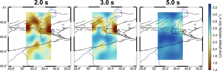
366                                                                               G. Taylor et al.: NAFZ surface wave tomography

Figure 2. Record section of correlation functions calculated for inter-station paths of the DANA network. Correlation functions were filtered
between 0.05 and 2.0 Hz and binned and stacked in 0.5 km distance bins, and the amplitude is normalized within each bin. Record sections
for every combination of three-component motion are labelled as follows: Z – vertical, R – radial, T – transverse. The ZR correlation (bottom
left) represents the motion recorded on the radial component due to a vertical point source. ZZ, ZR, RR and RZ components show Rayleigh
waves, and TT shows Love waves.

correlations into the relevant great circle path (station to sta-        terpreted. While these waveforms can be used for imaging
tion) to retrieve the vertical, radial and transverse correlation        (e.g. Hillers et al., 2016; Taylor et al., 2016), we focus here
components (Fig. 2). The correlation functions in Fig. 2 are             on the propagating surface waves that dominate the record
stacked in bins of 0.5 km inter-station distance and bandpass            sections. Correlations between the vertical and radial compo-
filtered between 0.05 and 2.0 Hz. The amplitudes are normal-             nents (ZZ, ZR, RR and RZ) predominantly contain Rayleigh
ized within each bin.                                                    waves propagating between DANA stations, whilst the trans-
                                                                         verse (TT) correlations contain Love waves. Figure 2 shows
2.2   Extraction of surface wave phase velocities                        some evidence for cross-talk between vertical and transverse
                                                                         components (ZT and TZ) in the form of low-amplitude co-
                                                                         herent waves, perhaps indicating the effects of anisotropy or
The record sections exhibit multiple features and arrivals.
                                                                         the scattering of waves off 3-D Earth structures. Linear ar-
There are two explanations for the large-amplitude features
                                                                         rivals that are most prominent at arrival times of ±10 s may
around t = 0. Firstly, they may represent the signature of the
                                                                         represent body wave reflections contained within the ambient
overlapping converging and diverging surface waves to form
                                                                         noise, but may also be an artefact produced by the GPS time
focal spots in the wave field (Hillers et al., 2016). A sec-
                                                                         synchronization of the seismic instruments (Lehujeur et al.,
ond possible explanation is teleseismic body wave energy
                                                                         2018).
that arrives at the stations at a near-vertical incidence angle.
                                                                            To create phase velocity dispersion curves for the study
When these arrivals are cross-correlated, the very small dif-
                                                                         region, we first create group velocity–period diagrams (Lev-
ferential travel times of the energy result in large amplitudes
                                                                         shin and Ritzwoller, 2001) for each stacked correlation func-
near the zero lag correlation time (Landès et al., 2010; Hillers
                                                                         tion between periods of 1.0 and 10.0 s (Fig. S3 in the Sup-
et al., 2013). The large amplitudes are particularly prominent
                                                                         plement) using the programme do_mft (Herrmann, 2013).
on the ZZ component. This phenomenon has been observed
                                                                         We then pick the dispersion curve for each correlation func-
in a previous ambient noise study in Turkey: Warren et al.
                                                                         tion manually. Due to a poorer signal-to-noise ratio on the
(2013) observed large zero-time amplitudes in their correla-
                                                                         ZZ component, Rayleigh wave dispersion measurements are
tion functions up to a distance of 80 km. Additionally, large-
                                                                         picked from the RR component correlations, whilst Love
amplitude waveforms near t = 0 are often observed in ambi-
                                                                         wave measurements are picked from the TT component. Ex-
ent noise correlation studies (e.g. Poli et al., 2012; Villaseñor
                                                                         amples of period–group velocity maps used for picking the
et al., 2007; Zheng et al., 2011) and are typically left unin-

Solid Earth, 10, 363–378, 2019                                                                       www.solid-earth.net/10/363/2019/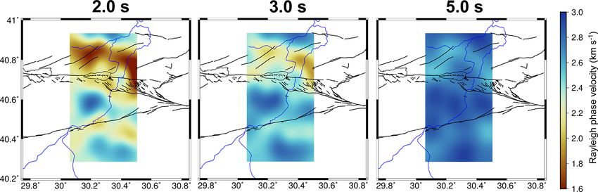
G. Taylor et al.: NAFZ surface wave tomography                                                                                  367

dispersion curves are shown in Supplement Fig. S3. Bensen           the average observed phase velocity at the given period. We
et al. (2007) suggest that in order for dispersion measure-         then invert the travel times for periods between 1.5 and 10.0 s
ments to be considered reliable, the station separation must        using the method of Rawlinson and Sambridge (2005). This
be greater than 3 wavelengths of the target wave. If we as-         is an iterative inversion, with each step consisting of calculat-
sume an average phase velocity of c = 3 km s−1 for the up-          ing travel times through the current phase velocity model by
per crust, our shortest-period surface waves of 1.5 s will have     wave-front tracking using the fast marching method (Sethian
a wavelength of 4.5 km. Thus, in order to satisfy the wave-         and Popovici, 1999). The inversion then seeks to minimize
length criterion, we discard all measurements with an inter-        the objective function:
station distance of 13.5 km or less as unreliable. For longer
periods and inter-station distances, for which some of the
                                                                    |g(m) − dobs |2 +  (m − m0 )T (m − m0 ) ,                   (2)
short-period data may be trustworthy, unreliable long-period
measurements are discarded based on visual inspection. This
also ensures that the large amplitudes of the near-zero ar-         where g(m) represents the travel times through the current
rivals do not contaminate our measurements from the later-          model, dobs represents the observed travel times from our
arriving surface waves. We use 62 stations in this study,           dispersion data,  is a variable damping factor, and m and
which amounts to a total of 1891 unique station pairs. As           m0 represent the current model and the starting model, re-
a result of the wavelength criterion, coupled with the visual       spectively. The variable damping term is included in order to
inspection of each period–velocity map, we retain measure-          minimize unconstrained model parameters (phase velocities)
ments from 929 station pairs for Rayleigh waves (49 % of            by preventing them from straying too far from our initial con-
the RR correlations) and 1173 station pairs for Love waves          stant velocity model. The choice of damping parameter, , is
(62 % of the TT correlations).                                      somewhat subjective. It should be selected with the aim of
   Phase velocity dispersion curves are also picked using           achieving a balance between the variance of the perturbations
do_mft (Herrmann, 2013). The phase velocity at each period          in the final phase velocity model with respect to the initial
is calculated from the previously picked group velocity by          model (a high variance indicates unrealistic values for un-
              ω0 r                                                  constrained model parameters) and obtaining a satisfactory
c=                           ,                               (1)    misfit to the observed travel time data. We constructed trade-
      −8 + π4 + ωU00r + N 2π
                                                                    off curves (Supplement Fig. S4) of final model perturbation
where 8 is the instantaneous phase of a narrow bandpass-            variance vs. final data misfit for both the Rayleigh and Love
filtered surface wave, ω0 is the centre frequency of the band-      wave inversions. We selected a damping factor of 40 s4 km−2
pass filter, r is the inter-station distance, U0 is the group ve-   for Rayleigh waves as it provided a 68 % reduction in the
locity and N is some integer. The N 2π term in Eq. (1) intro-       perturbation variance of the final model parameters (0.025 to
duces an ambiguity in the calculation of the phase velocity.        0.008 (km s−1 )2 ) for only a 2 % increase in data misfit (795 to
To overcome this ambiguity, do_mft (Herrmann, 2013) uses            815 ms) at a 4 s period. Likewise, for Love waves we choose
Eq. (1) to generate a suite of dispersion curves corresponding      a damping parameter of 60 s4 km−2 , which provides a 75 %
to different values of N. To pick the correct phase velocities,     reduction in final model variance (0.055 to 0.014 (km s−1 )2 )
we calculate the theoretical dispersion curve using an a priori     for an 8 % increase in misfit (670 to 730 ms). Increasing the
seismic velocity model of the region (Karahan et al., 2001)         damping parameter above these values leads to an increase
and manually pick the calculated dispersion curve (Eq. 1)           in misfit to the observed data which we find unacceptable.
that most closely corresponds to the theoretical dispersion         These constant damping factors are applied to the inversions
curve.                                                              at every period (Figs. 3 and 4).
                                                                       We do not include a separate smoothing parameter in our
2.3    Phase velocity tomography                                    inversion scheme, as a similar effect can be obtained by sim-
                                                                    ply reducing the number of model parameters and control-
After picking phase velocity dispersion curves for all inter-       ling the inversion through a damping parameter as described
station pairs for both Rayleigh and Love waves, we convert          above (Rawlinson and Sambridge, 2003). We have designed
the phase velocity at each period into a travel time between        our model discretization so that our velocity node separa-
the stations. We then use these travel time observations to         tion is comparable to our station separation, which should
invert for phase velocity as a function of position at each dis-    be a sufficiently coarse parameterization to constrain all our
crete period. We discretize each model as a 2-D grid of phase       model parameters and produce a smooth final model.
velocity nodes. The phase velocity tomography is carried out           The minimization of the objective function is performed
in a spherical coordinate system (Rawlinson and Sambridge,          using an iterative subspace inversion approach (Kennett
2005), with the node spacing (6.6 km in latitude and 7.6 km         et al., 1988), which projects the objective function onto a
in longitude) comparable to the average horizontal separation       multidimensional subspace of the data and model parame-
of the stations of the DANA network. We begin each inver-           ters. After 10 iterations the data misfit does not improve ap-
sion with a constant velocity model, with the velocity set to       preciably with further iterations, and the inversion is judged

www.solid-earth.net/10/363/2019/                                                                  Solid Earth, 10, 363–378, 2019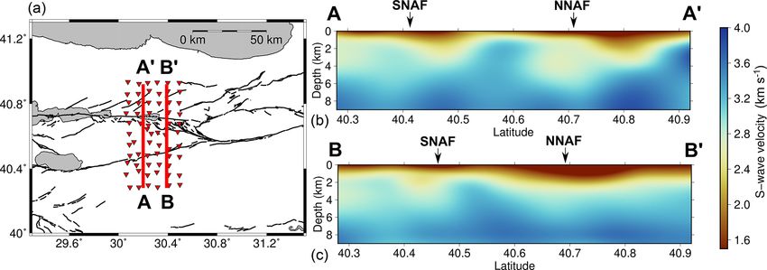
368                                                                              G. Taylor et al.: NAFZ surface wave tomography

Figure 3. Rayleigh wave phase velocity maps at 2.0, 3.0 and 5.0 s periods. Black lines show the mapped faults. The blue line represents the
Sakarya River flowing towards the north.

Figure 4. Love wave phase velocity maps at 2.0, 3.0 and 5.0 s periods. Black lines show the mapped faults. The blue line represents the
Sakarya River flowing towards the north.

to have converged. Stable solutions are shown in Figs. 3 and            location is defined for the neighbourhood algorithm as
4 for periods of 2.0, 3.0 and 5.0 s.                                          v
                                                                              u nf
                                                                              uX (vdi − vmi )2
                                                                        φm = t            2n
                                                                                                   ,                                   (3)
                                                                                 i=1     vdi  f
2.4   S-wave velocity inversion
                                                                        where nf is the number of frequencies in the dispersion curve,
                                                                        vdi is the observed phase velocity at frequency i from our to-
After obtaining 2-D maps of phase velocity for all periods              mographic model and vmi is the phase velocity at that fre-
between 1.5 and 10.0 s, the resulting dispersion relation at            quency inferred from the inverted S-wave model. Models
each node on the same geographic grid was inverted to ob-               that fit the dispersion curves extracted from the phase ve-
tain isotropic S-wave velocity as a function of depth at that           locity tomography with φm < 0.25 (Eq. 3) were used in a
location. Both Rayleigh and Love wave dispersion data are               weighted average to construct an initial estimate for S-wave
inverted together, with equal weighting, in order to obtain an          velocity vs. depth. Examples of the distribution of models
S-wave velocity model that best satisfies both data sets. The           used in the weighted average at three grid points, one each in
initial inversion was performed using a neighbourhood al-               the Sakarya Terrane, Armutlu Block and Istanbul zone, are
gorithm (Sambridge, 1999b; Wathelet, 2008) parameterized                shown in Fig. 5. The weighting of each model is the inverse
by a model consisting of 10 layers with variable layer thick-           of its misfit to the dispersion data as described in Eq. (3).
ness and S-wave velocity. The total number of free parame-                 This average model was then used as the starting model
ters is 20. The S-wave velocity of each layer is permitted to           for a linearized iterative inversion scheme as implemented
vary with a uniform distribution between 0.5 and 4.5 km s−1 ,           in surf96 (Herrmann, 2013). The inversion was judged to
whilst layer thickness could vary between 0.5 and 1.5 km.               have converged once the root mean square change in the
An increase in S-wave velocity with layer depth is also pre-            S-wave velocity model between iterations was negligible
scribed. The neighbourhood algorithm was allowed to run                 (< 0.1 km s−1 ), usually within six iterations. The set of 1-
until 20 050 different S-wave velocity models had been gen-             D models obtained from the linearized inversion represents
erated for each node in the grid. The misfit parameter at each          our 3-D S-wave velocity model for the region.

Solid Earth, 10, 363–378, 2019                                                                     www.solid-earth.net/10/363/2019/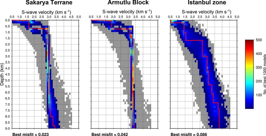
G. Taylor et al.: NAFZ surface wave tomography 369
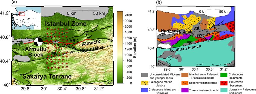
Figure 5. Results of the neighbourhood algorithm inversion for S-wave velocity at three nodes in the different geological units (Fig. 1).
The grey region represents the range of accepted models with a misfit below 0.25 (Eq. 3). The coloured region shows the range of the 1000
models with the lowest misfit. Red colours indicate a higher number of the best 1000 models with a certain S-wave velocity at that depth.
The solid red line shows the best-fitting model, the misfit of which is shown at the bottom of each panel. The location of each of these nodes
is shown in Fig. 6.
The advantage of the neighbourhood algorithm is that it olution of the inversion (Figs. S9 and S10). The initial and
provides a much broader overview of the acceptable param- final data misfit of the tomography models for both Rayleigh
eter space for our S-wave velocity model, rather than invert- and Love wave phase velocities are shown in Supplement
ing for a single model that best fits the data. The output of the Figs. S5 and S6. The significant reduction in the variance of
neighbourhood algorithm (Fig. 5) also allows for an intuitive, the travel time residuals in the final models, on average about
if qualitative, understanding of potential uncertainty in our 50 %, indicates that the final models better account for struc-
final S-wave velocity model. A disadvantage of the neigh- tural heterogeneity. Similarly, the higher variance of the final
bourhood algorithm is that only a relatively small number travel time residuals at shorter periods indicates stronger het-
of model parameters can be included in the inversion (∼ 30) erogeneity at shallow depths or noisier phase velocity mea-
before the parameter space becomes too large to search effi- surements at these periods.
ciently (Sambridge, 1999a). This means that the neighbour-
hood algorithm can only constrain relatively simple models. 3.1 Rayleigh wave phase velocity
For these reasons, we present the results of the neighbour-
hood algorithm (Fig. 5), but also perform a linearized inver-
Figure 3 shows the results of the Rayleigh wave phase veloc-
sion (Herrmann, 2013) to obtain a final model that better fits
ity tomography for periods between 2.0 and 5.0 s. The most
the data overall. This approach has been used previously in
interesting features of the velocity model include the large
fault zone imaging (Hillers and Campillo, 2018) and attempts
low-velocity (1.5–2.0 km s−1 ) anomaly located north of the
to strike a balance between presenting a model that satis-
northern branch of the NAFZ. These low velocities are likely
fies the data and gives a broader overview of the acceptable
due to the deep sedimentary basin at Adapazari in the north-
model space that is not available when using only a linearized
eastern part of the model and heavily faulted sediments near
inversion scheme.
Izmit in the north-western sector (Sengör et al., 2005). Be-
tween the two fault strands, the Armutlu Block can be seen
3 Results as a prominent region of high phase velocity (∼ 3.0 km s−1 ),
likely associated with the metamorphic rocks and possible
In this section, we describe the phase velocity maps de- granitic intrusions that exist in this region (Bekler and Gur-
rived separately for Rayleigh and Love wave travel time buz, 2008; Sengör et al., 2005). At 2.0 and 3.0 s periods, this
data. Sensitivity kernels representing the vertical resolution high-velocity region is particularly prominent in the western
for Rayleigh and Love waves within our period range can part of the Armutlu Block (Fig. 3). At a 5.0 s period, the en-
be found in the Supplement (Fig. S8), along with synthetic tire Armutlu Block consists of high velocities. At a 2.0 s pe-
checkerboard recovery tests to illustrate the horizontal res- riod, the sediments of the Pamukova basin can be seen along
www.solid-earth.net/10/363/2019/ Solid Earth, 10, 363–378, 2019370 G. Taylor et al.: NAFZ surface wave tomography
the southern branch of the NAFZ with velocities of approxi- possibly conflicting constraints on the model velocity pro-
mately 2.0 km s−1 . To the south, in the Sakarya Terrane, a rel- file. To improve the data misfit in such cases, a linearized
atively high-velocity anomaly (faster than 2.5 km s−1 ) can be inversion approach with surf96 (Herrmann, 2013) is used to
seen at all periods greater than 2.0 s. These velocities are in find an optimum model. Supplement Fig. S7 shows the final
general higher than those observed in the part of the Istanbul fit of the dispersion curves calculated at each of the nodes
zone that bounds the fault, and they likely indicate the crys- shown in Fig. 5. The dispersion curves were calculated for
talline basement of the Sakarya Terrane at shallower depths, the final S-wave velocity model and compared to dispersion
with thinner sedimentary cover. It is likely that the high phase curves extracted from the Rayleigh and Love wave phase
velocities observed in the far north of the model correspond velocity tomography. Supplement Fig. S7 also summarizes
to the older sedimentary units and crystalline rocks of the Is- the improvement in the misfit to the dispersion data provided
tanbul zone that underlie the clastic sediments at Izmit and by employing the linearized inversion (Herrmann, 2013) af-
Adapazari (Okay et al., 1994). In general, at a 5.0 s period or ter the neighbourhood algorithm. Each node has a signifi-
lower, the contrast in phase velocity between the major tec- cant improvement in misfit following the linearized inversion
tonic units is relatively low. This is likely due to the longer (> 50 %).
wavelength of these waves, which will average lateral varia-
tions in structure at these larger periods. 3.4 Isotropic S-wave velocity maps
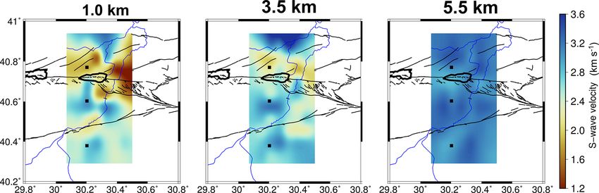
3.2 Love wave phase velocity Figure 6 shows depth slices through the final S-wave veloc-
ity model at depths of 1.5, 3.5 and 5.5 km. The final S-wave
The Love wave phase velocity images (Fig. 4) show a very velocity model is produced by performing a minimum cur-
similar pattern to the Rayleigh wave images. To the north of vature interpolation between our model nodes, which have
the fault extremely low (∼ 1.2 km s−1 ) phase velocities are the same spacing as our phase velocity model (Sect. 2.3).
associated with the faulted sediments near Izmit, as well as In the top 3 km of the crust we observe low S-wave veloci-
the Adapazari basin. Both of these features are visible for pe- ties (1.6–2.0 km s−1 ) on the north side of the northern fault
riods < 5.0 s. Low velocities also seem to be strongly asso- strand, associated with the Adapazari basin and faulted sed-
ciated with the NW–SE-striking faults just north of the rup- iments near Izmit. These low S-wave velocities are not ob-
ture zone of the Izmit earthquake at 40.7◦ N and 30.45◦ E. served at model depths of 3.5 km and below (Fig. 7), indicat-
Focal mechanisms for earthquakes in this region show exam- ing that the Adapazari basin is likely not deeper than about
ples of normal faulting (Altuncu Poyraz et al., 2015), indicat- 3.5 km. At 5.5 km of depth, relatively low S-wave velocities
ing these low velocities could be associated with a releasing (2.8 km s−1 ) are clearly associated with the northern branch
bend on the northern branch. The Armutlu Block between of the NAFZ, particularly within the zone of the Izmit rup-
the two fault strands shows high phase velocities exceeding ture beneath Lake Sapanca at 40.7◦ N and 30.2◦ E. Faster S-
2.4 km s−1 , which is comparable with those of the Rayleigh wave velocities, up to 3.5 km s−1 , are observed within the
wave images. The Pamukova basin can be seen for periods Armutlu Block between the two strands of the NAFZ. As
< 5.0 s near the southern branch of the fault with velocities with the phase velocity maps, these high velocities are more
of 1.5–2.5 km s−1 . At a 5.0 s period, higher phase velocities prominent west of the Sakarya River to a depth of about
(> 3.0 km s−1 ) are observed within the southern portion of 3.5 km. The slow velocities associated with the Pamukova
the Sakarya Terrane and the northern part of the Istanbul basin along the southern branch of the NAFZ are much at-
zone. These high velocities are again interpreted to represent tenuated at 3.5 km of depth, indicating that this basin is shal-
the crystalline basement of these tectonic units. As with the lower than the Adapazari basin. We observe evidence in the
Rayleigh wave phase velocity maps (Fig. 3), the lateral res- southern part of the model for crystalline rocks below a depth
olution of the Love wave images decreases with increasing of 1.5 km in the Sakarya Terrane, where S-wave velocities
period. exceed 2.5 km s−1 . These high velocities are also observed
in the far north of the model within the Istanbul zone. Both
3.3 S-wave velocity model misfit the northern and southern branches of the NAFZ appear to
exploit the regions where we observe high gradients in seis-
In order to construct an isotropic S-wave velocity profile at mic S-wave velocity. Both branches of the main fault skirt the
each node a two-step inversion process was chosen, as de- edges of the high-velocity zone associated with the Armutlu
scribed in Sect. 2.4. Examples of the results of the neigh- Block.
bourhood algorithm from three locations in the Sakarya Ter-
rane, Armutlu Block and Istanbul zone are shown in Fig. 5. 3.5 Isotropic S-wave velocity vertical profiles
The best 1000 models from the neighbourhood algorithm oc-
cupy a much smaller range for the Sakarya Terrane and Ar- Figure 7 shows two vertical sections through the S-wave ve-
mutlu Block examples. The broader range for the Istanbul locity model along a north–south profile located at 30.2◦ E
zone example shows that the data here provide weaker or (profile A–A0 ) and 30.4◦ E (profile B–B0 ). In profile A–A0
Solid Earth, 10, 363–378, 2019 www.solid-earth.net/10/363/2019/G. Taylor et al.: NAFZ surface wave tomography 371
Figure 6. Isotropic S-wave velocity maps at 1.5, 3.5 and 5.5 km of depth. Black lines show the mapped faults. The blue line represents the
Sakarya River flowing towards the north. The black squares represent the locations of the nodes shown in Fig. 5.
the low-velocity zone associated with the heavily faulted sed- where u0 is the average (isotropic) phase velocity. A is the
iments near Izmit (40.82◦ N) can be observed to a depth of amplitude of the 2θ term, which describes an azimuthal vari-
∼ 3.5 km, as can the Adapazari basin along profile B–B0 . In ation with 180◦ periodicity. φ2 is the fast direction of the 2θ
profile A–A0 the Armutlu Block is clearly distinguishable as term. B is the amplitude of the 4θ term, which has 90◦ peri-
a region of high velocity (∼ 2.8 km s−1 ) extending towards odicity, and φ4 is the corresponding fast direction.
the surface between 40.5 and 40.6◦ N. It is clear that high- The azimuthal variation of the raw Rayleigh wave phase
velocity metamorphic rocks found in this region (Yılmaz velocity measurements between 2.0 and 8.0 s periods is
et al., 1995) are located closer to the surface than the base- shown in Fig. 8. Figure 9 shows the variation of fast di-
ment rocks of the Sakarya Terrane and Istanbul zone. In both rection and magnitude of anisotropy for all periods between
profiles, a zone of low velocity (∼ 2.8 km s−1 ) can be seen 1.5 and 10.0 s. Although there is considerable variability in
extending to a depth of at least 6 km beneath the location of the individual phase velocities, there is a robust dependence
the surface expression of the northern branch of the NAFZ. of phase velocity on propagation direction that is observed
This low-velocity zone appears to be of the order of 10 km when averaging velocities in 5◦ azimuth bins. Figure 9 shows
wide (40.65 to 40.75◦ N). Low velocities associated with the a smooth variation in the fast direction with an increasing
southern branch of the fault zone are less clear, particularly period of the wave. At short periods (2–3 s) the fast direc-
for the eastern profile B–B0 , but are evident to 5 km of depth tion is aligned close to 90◦ from north, but changes smoothly
beneath profile A–A0 . However, it is difficult to distinguish to ∼ 50–70◦ from north above a 5 s period. Below 2 s peri-
the southern branch of the fault from the surrounding sedi- ods, the anisotropy has a magnitude greater than 1 %, but this
mentary cover of the Sakarya Terrane and Pamukova basin. magnitude decreases substantially between 2 and 4 s periods,
before increasing again at periods greater than 4.0 s to a value
3.6 Azimuthal anisotropy of ∼ 3 %.
In general, the amplitude of the 4θ term is at least 50 %
In order to quantify the level of azimuthal anisotropy in our lower than the 2θ term, which is to be expected for Rayleigh
phase velocity data set, we plot our raw phase velocity mea- waves (Smith and Dahlen, 1973). The exception to these
surements against the azimuth of the propagation direction trends is at 2.0 s periods. Here, the fast directions do not align
(from north). To reduce the scatter in the data and provide with those observed at longer periods, and the 4θ component
a meaningful measurement, we bin all of our phase velocity has twice the amplitude of the 2θ component. However, both
measurements by azimuth with a bin size of 5◦ . The phase the RMS misfit and the variance of the residuals between the
velocities within each bin are averaged to provide a mean observed data and Eq. (4) are much greater at 2.0 s periods,
measurement and a corresponding standard error. Rayleigh as is the case with the phase velocity tomography. In partic-
and Love wave observations are treated separately. Due to ular, the greater variance of the residuals implies a greater
the presumed symmetry of propagation velocity in both di- uncertainty in the data fit. Greater variance in the 2.0 s phase
rections between pairs of stations, our measurements are in velocities is likely due to the fact that waves at 2.0 s periods
an azimuth range of 0 to 180◦ . We attempt to fit the binned are more sensitive to short-wavelength heterogeneities near
data at each period with the following function to describe the surface.
the azimuthal variation of phase velocity (Smith and Dahlen, A further source of uncertainty in our calculation of az-
1973): imuthal anisotropy is the unknown noise source distribution
of the region. It is clear from the azimuthal distribution of
our phase velocity measurements (Figs. S17 and S18 in the
c(θ ) = u0 + A cos(2(θ − φ2 )) + B cos(4(θ − φ4 )), (4)
www.solid-earth.net/10/363/2019/ Solid Earth, 10, 363–378, 2019372 G. Taylor et al.: NAFZ surface wave tomography Figure 7. (a) Map of the Izmit–Adapazari region showing station locations of the DANA network as red triangles and mapped faults as black lines. Thick red lines indicate the location of the vertical profiles taken through the S-wave velocity model along lines A–A0 and B–B0 . (b) Vertical S-wave velocity profile between A and A0 . (c) Vertical S-wave velocity profile between B and B0 . The profiles show S-wave velocity between the surface and 9 km of depth. The approximate locations of the surface traces of the northern and southern branches of the NAFZ are indicated by NNAF and SNAF, respectively. Figure 8. Azimuthal variation of Rayleigh wave phase velocities with propagation azimuth (from north). Black dots indicate the raw phase velocity measurements, and large red dots show the average of the phase velocities within 5◦ azimuth bins and the corresponding standard error of the mean for the bin. The blue line is the best-fitting curve (Eq. 4) to the binned data (red dots). u0 is the average (isotropic) phase velocity. We show the root mean square misfit of the blue curve to the phase velocity measurements, as well as the variance of the residuals. We indicate the 2θ and 4θ amplitudes and fast directions that correspond to the blue curve. The azimuthal distribution of ray paths used in this analysis is shown in Supplement Fig. S14. Supplement) that there is a possible bias due to the number of display a higher standard error of the mean than those for ray paths that are oriented north–south. Fewer observations north–south-oriented ray paths (0 or 180◦ ). are available for ray paths that are not aligned in the dominant The azimuthal anisotropy of the Love wave phase ve- direction, leading to higher uncertainty in our measurements locities is shown in Supplement Fig. S13. The Love wave of anisotropy. This effect is visible in Fig. 8: measurements anisotropy is less clear. In general, the 2θ fast direction lies taken from east–west-oriented ray paths (∼ 90◦ ) generally between 25 and 40◦ from north. The 4θ fast direction is more Solid Earth, 10, 363–378, 2019 www.solid-earth.net/10/363/2019/
G. Taylor et al.: NAFZ surface wave tomography                                                                                        373

                                                                          nal S-wave velocity models at the three locations specified in
                                                                          Fig. 6.
                                                                             Our tomographic models show that both the northern and
                                                                          southern branches of the NAFZ have exploited boundaries
                                                                          between major lithological units. In particular, the metamor-
                                                                          phic rocks of the Armutlu Block are clearly mapped due to
                                                                          the strong velocity contrast with rocks of the Istanbul zone to
                                                                          the north and the Sakarya Terrane to the south (Figs. 3, 4 and
                                                                          6).
                                                                             Seismic velocity models of the crust in this region have
                                                                          also been constructed from teleseismic body wave tomog-
                                                                          raphy by Papaleo et al. (2017, 2018). They image depth-
Figure 9. Variation of 2θ Rayleigh wave anisotropy with period in         averaged seismic velocity between the surface and 90 km of
the Izmit–Adapazari region. The red dots are the measured magni-          depth, with a vertical and horizontal resolution of ∼ 15 km
tude of anisotropy at each period, and the corresponding uncertainty      (Papaleo et al., 2017, 2018). Despite the large difference in
is the standard deviation of the anisotropy magnitude taken from          model resolution and a non-overlapping depth range, Papa-
the covariance matrix during the curve-fitting process described in       leo et al. (2017, 2018) detect reduced crustal seismic veloc-
Sect. 3.6. The black lines indicate the angle from north of the 2θ fast   ities immediately to the north of the NAFZ, in the same re-
direction at each period, and the top of the plot represents north.       gions we observe low S-wave velocities associated with the
                                                                          Adapazari basin, and heavily faulted sedimentary cover in
                                                                          the north-western part of the array (Figs. 6 and 7). Low P-
variable, mostly lying between 85 and 120◦ . The average                  wave velocities observed by Papaleo et al. (2017) are also co-
amplitude of the 2θ term is 0.036 km s−1 . Whilst the am-                 located with the low S-wave velocities detected in this study
plitude of the 4θ term is more comparable in amplitude to                 beneath the Pamukova basin. Papaleo et al. (2017, 2018) also
the 2θ term than for the Rayleigh waves, it is still consis-              found relatively high seismic velocity at depth within the Ar-
tently smaller, with an average of 0.024 km s−1 . The RMS                 mutlu Block. We detect high S-wave velocities much closer
misfit and variance of the residuals are again higher at the              to the surface that we attribute to the shallow metamorphic
shorter periods of 2.0 and 4.0 s, again indicating sensitivity to         rocks reported in this region (Yılmaz et al., 1995). We note
shorter-wavelength structural complexities near the surface.              that the relatively high seismic velocities we find in the upper
The azimuthal distribution of ray paths used in this analysis             crust of the Armutlu Block also correspond to a region of rel-
is shown in Supplement Figs. S14 and S15.                                 atively low electrical resistivity found by Tank et al. (2005)
                                                                          in the upper 10 km.
                                                                             The depth of sedimentary cover of the Adapazari basin has
4     Discussion                                                          been estimated to be at least 1.0 km in some locations (Ko-
                                                                          mazawa et al., 2002). These estimates were made by invert-
4.1    S-wave velocity model                                              ing Rayleigh wave phase velocity measurements from mi-
                                                                          croseisms recorded at two arrays within the basin. Due to
The horizontal resolution of the S-wave velocity model at                 a lack of measurements below 0.6 Hz (>∼ 1.6 s period) the
depth in Fig. 7 is limited by the wavelength of the surface               inversion of Komazawa et al. (2002) assumed an S-wave ve-
waves used in this study. Receiver function and autocorrela-              locity of 3.5 km s−1 below a depth of 500 m in the basin. Our
tion studies of the region show that the shear zone associated            velocity model, which incorporates Rayleigh wave observa-
with the NAFZ is perhaps no wider than ∼ 7 km through the                 tions up to a 10.0 s period, indicates that S-wave velocity may
crust and into the upper mantle (Kahraman et al., 2015; Tay-              be no greater than 3.0 km s−1 up to a depth of 2.5 km within
lor et al., 2016). In the upper crust, the main fault strands             the basin. Our measurements therefore imply that the Ada-
are estimated to be no more than a few kilometres wide in                 pazari basin could have a depth of up to 2.5 km based on the
this region (Okay and Tüysüz, 1999). Low S-wave velocities                observed increase in S-wave velocity at this depth. Similarly,
associated with the northern branch of the NAFZ are observ-               the Pamukova basin may be as deep as 2.5 km, though it is
able in our model down to a depth of 6 km. Below this depth,              difficult to accurately detect the depth to material interfaces
we rely on observations derived from Rayleigh waves with a                using only surface wave observations.
period greater than 8.0 s (phase velocity sensitivity kernels in             Studies of the near-surface structure of the San Jacinto
Supplement Fig. S8). Assuming a phase velocity of 3 km s−1 ,              Fault zone in southern California (Allam and Ben-Zion,
these waves have a wavelength of ∼ 24 km. Thus, we can-                   2012; Zigone et al., 2015) observe prominent “flower struc-
not expect to resolve such a narrow structure at depth unless             tures” associated with the fault. These structures are zones of
it offsets rocks of differing seismic velocity. In the Supple-            low seismic velocity that are wide near the surface, become
ment (Fig. S9), we include the resolution kernels of the fi-              narrower with depth and are interpreted to be a damage zone

www.solid-earth.net/10/363/2019/                                                                       Solid Earth, 10, 363–378, 2019
374 G. Taylor et al.: NAFZ surface wave tomography created during fault propagation through undeformed crust. 4.2 Azimuthal anisotropy The surface wave analysis does not enable us to observe a narrowing with depth of the low-velocity zone associated The 2θ and 4θ fast directions for Rayleigh waves vary be- with the northern branch of the NAFZ in Fig. 7. Nonethe- tween 50 and 90◦ from north (Fig. 9), whilst Love wave 2θ less, the low-velocity anomalies associated with the Ada- fast directions vary from 20 to 40◦ from north (Fig. S13). pazari and Izmit regions might be interpreted as crust that The Love wave 4θ fast direction is highly variable, with no has been damaged by movement on and around the northern distinct pattern that can be readily observed. strand of the fault. It is clear that the strongest contrasts in Our observations of azimuthal anisotropy are complemen- seismic velocities in our model (Figs. 3, 4 and 6) are asso- tary to the observations of previous studies along the North ciated with boundaries among the three main tectonic units. Anatolian Fault. Two studies of shear wave splitting mea- The North Anatolian Fault zone appears to have developed surements of the Karadere–Düzce segment (∼ 50 km east of along pre-existing tectonic boundaries. the current study region) by Peng and Ben-Zion (2004, 2005) Such seismic velocity contrasts across an active strike-slip also display a seismic fast direction in the upper crust that fault are also present in California on the creeping section of clusters between 45 and 90◦ from north, often aligning par- the San Andreas Fault to the north of Parkfield where the allel to the strike of the North Anatolian Fault. Further shear fault trace is located along a strong seismic velocity con- wave splitting measurements made by Hurd and Bohnhoff trast between the Great Valley sedimentary sequence and (2012) at the station CAY, located within our study region to the granites of the Salinian terrane (Eberhart-Phillips and the east of Lake Sapanca (Fig. 1), also showed fast directions Michael, 1993; Thurber et al., 2006). This phenomenon is between 30 and 90◦ , with the majority falling between 40 and also observed across the Hayward fault near San Francisco 50◦ . Further east, the fast polarization directions measured where there is a clear seismic velocity contrast between the by Hurd and Bohnhoff (2012) are more commonly aligned Great Valley sequence and the Franciscan Complex (Harde- NW–SE. beck et al., 2007; Thurber et al., 2006). Eberhart-Phillips and There are two possible mechanisms of crustal anisotropy: Michael (1993) suggest that the San Andreas Fault is likely to stress controlled or structure controlled. If the anisotropy is creep in sections in which this clear velocity contrast exists, stress controlled, it is expected that the fast direction will whilst being locked and rupturing seismogenically where align with the direction of maximum horizontal compres- the velocity contrast across the fault is less defined. How- sion in the stress field due to the closure of cracks on the ever, this association between a creeping fault segment and a perpendicular direction (Crampin and Lovell, 1991). For an clearly defined velocity contrast evidently does not hold for east–west-striking fault, this would result in an expected fast this section of the NAFZ where the 1999 Izmit and Düzce direction aligned NW–SE, or 120–160◦ from north (Bohn- earthquakes occurred. Furthermore, a recent geodetic study hoff et al., 2006). Our observations, and those of previous found evidence of only low creep rates on this segment, prob- studies (Peng and Ben-Zion, 2004, 2005), show that this is ably related to earthquake after-slip at shallow depths (Hus- not the case, at least for stations located close to the fault. A sain et al., 2016). dominant fast direction between 50 and 90◦ (NE–SW) from The relatively high S-wave velocities we observe within north (Fig. 9) indicates that the anisotropy in the region is the Armutlu Block likely indicate metamorphic rocks and likely structure controlled. This observation was also noted pre-Jurassic basement (Akbayram et al., 2016), the surface in anisotropic receiver functions by Licciardi et al. (2018), outcrops of which are of unknown provenance and age (Okay who found that the fast shear wave polarization directions and Tüysüz, 1999). This metamorphic unit within the Ar- along the central portion of the North Anatolian Fault align mutlu Block is evidently resistant to strain, which is de- with the strike of mapped faults at stations located close to flected onto the northern and southern branches of the NAFZ those faults, implying structure-controlled anisotropy. that bound this high S-wave velocity region. This behaviour Figure 9 shows a nearly 90◦ fast direction at a 2–3 s pe- is also observed in the near-surface structure of the south- riod (depths of ∼ 0–3 km) that aligns approximately with the eastern section of the Alpine Fault on South Island, New strike of the North Anatolian Fault through the region. This Zealand, where the fault trace is located at the edge of the observation clearly implies structure-controlled anisotropy metamorphic Haast Schist and cuts through thick coastal that is dominated by faulting in the very upper crust, similar sediments (Eberhart-Phillips and Bannister, 2002). Fichtner to the observations of Licciardi et al. (2018) for the top 15 km et al. (2013) image the S-wave velocity structure of the up- of the central section of the North Anatolian Fault. At periods per mantle beneath the NAFZ using full waveform inversion. greater than 4.5 s (Fig. 9), our observed fast direction does At this much larger length and depth scale, they also note not systematically align with any of the mapped faults in the that the NAFZ appears to be bounded by tectonic blocks of region (Fig. 1). Instead, the fast direction at these periods is high seismic velocity. They interpret this as evidence that the better compared to the 45◦ direction of maximum extension fault zone developed along the edges of high-rigidity blocks, for the Izmit–Adapazari region calculated from inter-seismic analogous to our observations for the near-surface structure GPS data by Allmendinger et al. (2007), and it is consis- of the Armutlu Block. tent with shear wave splitting measurements from the central Solid Earth, 10, 363–378, 2019 www.solid-earth.net/10/363/2019/
G. Taylor et al.: NAFZ surface wave tomography                                                                                   375

portion of the North Anatolian Fault made by Biryol et al.        sistent with the Sakarya Terrane being an accretionary com-
(2010), who found a fast polarization direction that varied       plex of sedimentary rocks overlying a metamorphic crys-
between 35 and 60◦ . Further analysis of shear wave splitting     talline basement (Yılmaz et al., 1995). Our analysis of the
results by Vinnik et al. (2016) show an average fast direction    azimuthal variation in phase velocities finds that regional
of ∼ 60◦ down to a depth of about 30 km.                          seismic anisotropy is likely structure controlled. At short pe-
   This close correspondence between the seismic fast direc-      riods, both Rayleigh and Love waves have a fast direction
tion and the direction of maximum extension implies that          which roughly aligns with the strike of the North Anato-
structure-controlled anisotropy is the result of mineral foli-    lian Fault (east–west), as opposed to the direction of max-
ation within the crust. Some minerals in upper crustal rocks,     imum compression (NW–SE). At longer periods (> 4.0 s),
such as micas and amphibole, typically have cleavage planes       the fast direction smoothly transitions from the maximum
or crystallographic axes aligned with the dominant strain di-     shear direction towards the principal extension direction of
rection and are the dominant source of anisotropy within the      the lithosphere (NE–SW), indicating that mineral fabric may
bulk rock (e.g. Kern and Wenk, 1990; Mainprice and Nico-          be the source of azimuthal anisotropy. Studying the relation-
las, 1989; Sherrington et al., 2004). These minerals are par-     ship among the three distinct tectonic units of the region, in-
ticularly common in high-grade metamorphic rocks, such as         cluding the patterns of seismic anisotropy, provides insight
slates and schists, and are likely abundant within the Armutlu    into the potential for strain localization along both the north-
Block. Analyses of samples of calcite and amphiboles taken        ern and southern branches of the NAFZ. This knowledge is
from the Uludag Massif (∼ 100 km south-west of Izmit–             critical to understanding the long-term behaviour of the fault
Adapazari) by Farrell (2017) show that the fast propagation       zone and the seismic hazard that it poses.
for both P and S waves aligns parallel to the foliation direc-
tion in these minerals. We therefore think it likely that the
seismic fast directions we observe at longer periods are de-      Data availability. The final S-wave velocity model of the Izmit–
termined by deformation fabrics aligned with the dominant         Adapazari region is included as an ASCII text file within the Sup-
shear regime.                                                     plement. Data for this study can be found at the IRIS Data Manage-
                                                                  ment Centre under network code YH (2012–2013) (DANA, 2012).

5   Conclusions
                                                                  Supplement. The supplement related to this article is available
                                                                  online at: https://doi.org/10.5194/se-10-363-2019-supplement.
We utilized the ambient noise field recorded at a tempo-
rary network in the Izmit–Adapazari region of north-western
Turkey to retrieve Rayleigh and Love waves propagating be-        Author contributions. GT performed the formal analysis, with the
tween the stations of the array. We performed surface wave        exception of the calculation of the raw cross-correlation functions,
phase velocity tomography, followed by an inversion for S-        under the supervision of SR, GAH and GH. GH calculated the raw
wave velocity structure, with waves of periods from 1.5 to        cross-correlation functions. GT prepared the paper with contribu-
10.0 s to image the shear wave velocity in the top 10 km of       tions from all co-authors. GH produced Supplement Figs. S1 and
the North Anatolian Fault zone.                                   S2.
   Our model shows low S-wave velocity to the north of the
NAFZ, associated with faulted marine clastic sediments near
Izmit (Akbayram et al., 2016) and with the Adapazari sedi-        Competing interests. The authors declare that they have no conflict
mentary basin, which we estimate to have a thickness of at        of interest.
least 2.5 km. Between the two branches of the NAFZ, we ob-
serve a high-velocity region linked to metamorphic and ig-
neous rocks in the Armutlu Block. It is likely that this high     Acknowledgements. George Taylor is supported by the Leeds–
S-wave velocity in the upper crust is indicative of a rheo-       York Doctoral Training Partnership of the Natural Environment
                                                                  Research Council (NERC), UK. Gregor Hillers acknowledges
logically strong region that preferentially localizes strain at
                                                                  support through a Heisenberg fellowship from the German Re-
the boundaries of the Armutlu Block, particularly along its       search Foundation (HI 1714/1-2). The DANA array was part of the
northern boundary, which has been identified as the Intra-        Faultlab project, a collaborative effort by the University of Leeds,
Pontide suture zone. We also image the Pamukova basin as a        Kandilli Observatory and Earthquake Research Institute, and
region of low S-wave velocity to a depth of about 2.5 km as-      Sakarya University. Major funding was provided by the UK NERC
sociated with the southern branch of the NAFZ. Both basins        under grant NE/I028017/1. Equipment was provided and supported
are likely related to pull-apart motion along the northern and    by the NERC Geophysical Equipment Facility (SEIS-UK) loan
southern branches of the NAFZ, where they are oblique to          947. We would like to thank Sven Schippkus and an anonymous
the principal shear direction.                                    reviewer for their detailed reviews that helped improve the paper.
   To the south of the NAFZ, we image the Sakarya Ter-
rane as a region of moderate to high S-wave velocity, con-

www.solid-earth.net/10/363/2019/                                                                 Solid Earth, 10, 363–378, 2019
You can also read