Partitioning of canopy and soil CO2 fluxes in a pine forest at the dry timberline across a 13-year observation period
←
→
Page content transcription
If your browser does not render page correctly, please read the page content below
Biogeosciences, 17, 699–714, 2020
https://doi.org/10.5194/bg-17-699-2020
© Author(s) 2020. This work is distributed under
the Creative Commons Attribution 4.0 License.

Partitioning of canopy and soil CO2 fluxes in a pine forest at the dry
timberline across a 13-year observation period
Rafat Qubaja, Fyodor Tatarinov, Eyal Rotenberg, and Dan Yakir
Department of Earth and Planetary Sciences, Weizmann Institute of Science, Rehovot 76100, Israel

Correspondence: Dan Yakir (dan.yakir@weizmann.ac.il)

Received: 25 July 2019 – Discussion started: 31 July 2019
Revised: 12 December 2019 – Accepted: 6 January 2020 – Published: 11 February 2020

Abstract. Partitioning carbon fluxes is key to understand-        1   Introduction
ing the process underlying ecosystem response to change.
This study used soil and canopy fluxes with stable isotopes       The annual net storage of carbon in the land biosphere,
(13 C) and radiocarbon (14 C) measurements in an 18 km2 , 50-     known as net ecosystem production (NEP), is the balance
year-old, dry (287 mm mean annual precipitation; nonirri-         between carbon uptake during gross primary productivity
gated) Pinus halepensis forest plantation in Israel to parti-     (GPP) and carbon loss during growth, maintenance respira-
tion the net ecosystem’s CO2 flux into gross primary pro-         tion by plants (i.e., autotrophic respiration, Ra ), and decom-
ductivity (GPP) and ecosystem respiration (Re ) and (with         position of litter and soil organic matter (i.e., heterotrophic
the aid of isotopic measurements) soil respiration flux (Rs )     respiration, Rh ; Bonan, 2008). The difference between GPP
into autotrophic (Rsa ), heterotrophic (Rh ), and inorganic       and Ra expresses the net primary production (NPP) and is the
(Ri ) components. On an annual scale, GPP and Re were             net carbon uptake by plants that can be used for new biomass
655 and 488 g C m−2 , respectively, with a net primary pro-       production. Measurements from a range of ecosystems have
ductivity (NPP) of 282 g C m−2 and carbon-use efficiency          shown that total plant respiration can be as large as 50 % of
(CUE = NPP / GPP) of 0.43. Rs made up 60 % of the Re and          GPP (e.g., Etzold et al., 2011) and together with Rh com-
comprised 24 ± 4 %Rsa , 23 ± 4 %Rh , and 13 ± 1 %Ri . The         prises total ecosystem respiration (Re ; Re = Ra + Rh ). The
contribution of root and microbial respiration to Re increased    partitioning of the ecosystem carbon fluxes can therefore be
during high productivity periods, and inorganic sources were      summarized as
more significant components when the soil water content was
low. Comparing the ratio of the respiration components to Re      GPP = NPP + Ra = NEP + Rh + Ra .                           (1)
of our mean 2016 values to those of 2003 (mean for 2001–
2006) at the same site indicated a decrease in the autotrophic    Earlier campaign-based measurements carried out by
components (roots, foliage, and wood) by about −13 % and          Maseyk et al. (2008a) and Grünzweig et al. (2009) in the
an increase in the heterotrophic component (Rh /Re ) by about     semiarid Pinus halepensis (Aleppo pine) Yatir Forest indi-
+18 %, with similar trends for soil respiration (Rsa /Rs de-      cated that GPP at this site was lower than among temper-
creasing by −19 % and Rh /Rs increasing by +8 %, respec-          ate coniferous forests (1000–1900 g C m−2 yr−1 ) but within
tively). The soil respiration sensitivity to temperature (Q10 )   the range estimated for Mediterranean evergreen needleleaf
decreased across the same observation period by 36 % and          and boreal coniferous forests (Falge et al., 2002; Flechard
9 % in the wet and dry periods, respectively. Low rates of        et al., 2019b) and had a high carbon-use efficiency (CUE)
soil carbon loss combined with relatively high belowground        of 0.4 (CUE = NPP / GPP; DeLucia et al., 2007). The to-
carbon allocation (i.e., 38 % of canopy CO2 uptake) and low       tal flux of CO2 released from the ecosystem (Re ) can be
sensitivity to temperature help explain the high soil organic     partitioned into aboveground autotrophic respiration (i.e., fo-
carbon accumulation and the relatively high ecosystem CUE         liage and sapwood, Rf ) and soil CO2 flux (Rs ). Rs , in turn,
of the dry forest.                                                is a combination of three principal components and can
                                                                  be further partitioned into the components originating from

Published by Copernicus Publications on behalf of the European Geosciences Union.
700                                                                R. Qubaja et al.: Partitioning of canopy and soil CO2 fluxes

roots or rhizospheres and mycorrhizas (i.e., Rsa ), from car-        highlight the sensitivity of carbon fluxes in semiarid Mediter-
bon respired during the decomposition of dead organic mat-           ranean ecosystems to the irregular seasonal and interannual
ter by soil microorganisms and macrofauna (Rh ; Bahn et              distribution of rain events (Poulter et al., 2014; Ross et al.,
al., 2010; Kuzyakov, 2006), and from pedogenic or anthro-            2012). While Rs is generally constrained by low SWC dur-
pogenic acidification of soils containing CaCO3 (Ri ; Joseph         ing summer months, abrupt and large soil CO2 pulses have
et al., 2019; Kuzyakov, 2006), which is expressed as                 been observed after rewetting the dry soil (Matteucci et al.,
                                                                     2015).
Re = Rs + Rf = [Rsa + Rh + Ri ] + Rf .                      (2)          The objectives were twofold: first, to obtain detail on par-
                                                                     titioning of the carbon fluxes in a semiarid pine forest to help
Previously published results show that the contribution of           explain the high productivity and carbon use efficiency re-
Rsa and Rh to Rs ranges from 24 % to 65 % and from 29 %              cently reported for this ecosystem (Qubaja et al., 2019) and
to 74 %, respectively, in forest soils in different biomes and       provide process-based information to assess the carbon se-
ecosystems (Binkley et al., 2006; Chen et al., 2010; Flechard        questration potential of such a semiarid afforestation system;
et al., 2019a; Frey et al., 2006; Hogberg et al., 2009; Subke et     and second, to combine this 2016 study with the results of a
al., 2011). Some studies reported significant proportions of         similar one at the same site in 2003 (mean values for 2001–
abiotic contribution to Rs , ranging between 10 % and 60 %           2006; Grünzweig et al., 2007, 2009) to obtain a long-term
(Martí-Roura et al., 2019; Ramnarine et al., 2012; Joseph            perspective across 13 years on soil respiration and its parti-
et al., 2019). However, most of these experiments were per-          tioning. We hypothesized that the high carbon-use efficiency
formed in boreal, temperate, or subtropical forests, and there       of the dry-forest ecosystem is associated with high below-
is a general lack of information on water-limited environ-           ground carbon allocation and relatively low decomposition
ments, such as dry Mediterranean ecosystems. Using both              rates and that the long-term trend associated with warming
13 C and CO / O ratios also showed that abiotic processes,           may be suppressed by the dry conditions.
              2    2
such as CO2 storage, transport, and interactions with sedi-
ments, can influence Rs measurements at such sites (Angert
et al., 2015; Carmi et al., 2013). Furthermore, root-respired        2     Materials and methods
CO2 can also be dissolved in the xylem water and carried
upward with the transpiration stream (Etzold et al., 2013).          2.1    Site description
   Rates of the soil–atmosphere CO2 flux (Rs ) have been al-
tered owing to global climatic change, particularly through          The Yatir Forest (31◦ 200 4900 N, 35◦ 030 0700 E; 650 m a.s.l.) is
changes in soil temperature (Ts ) and soil moisture (SWC;            situated in the transition zone between subhumid and arid
Bond-Lamberty and Thomson, 2010; Buchmann, 2000; Car-                Mediterranean climates (Fig. S1 in the Supplement) on the
valhais et al., 2014; Hagedorn et al., 2016; Zhou et al., 2009),     edge of the Hebron mountain ridge. The ecosystem is a semi-
which could account for 65 %–92 % of the variability of Rs in        arid pine afforested area established in the 1960s and cover-
a mixed deciduous forest (Peterjohn et al., 1994). Soil mois-        ing approximately 18 km2 . The average air temperatures for
ture impacts on Rs have been observed in arid and Mediter-           January and July are 10.0 and 25.8 ◦ C, respectively. Mean
ranean ecosystems, where Ts and SWC are negatively corre-            annual potential evapotranspiration (ET) is 1600 mm, and
lated (e.g., Grünzweig et al., 2009). CO2 efflux generally in-       mean annual precipitation is 287 mm. Only winter (Decem-
creases with increasing soil temperatures (Frank et al., 2002),      ber to March) precipitation occurs in this region, creating
which can produce positive feedback on climate warming               a distinctive wet season, while summer (June to October)
(Conant et al., 1998), converting the biosphere from a net car-      is an extended dry season. There are short transition peri-
bon sink to a carbon source (IPCC, 2014). A range of empiri-         ods between seasons, with a wetting season (i.e., fall) and
cal models have been developed to relate Rs rate and temper-         a drying season (i.e., spring). The forest is dominated by
ature (Balogh et al., 2011; Lellei-Kovács et al., 2011), and the     Aleppo pine (Pinus halepensis Mill.), with smaller propor-
most widely used models rely on the Q10 approach (Bond-              tions of other pine species and cypress and little understory
Lamberty and Thomson, 2010), which quantifies the sensi-             vegetation. Tree density in 2007 was 300 trees ha−1 ; mean
tivity of Rs to temperature and can integrate it with physical       tree height was 10.0 m; diameter at breast height (DBH) was
processes, such as the rate of O2 diffusion into and CO2 dif-        ∼ 15.9 cm, and the leaf area index (LAI) was ∼ 1.5. The na-
fusion out of soils and the intrinsic temperature dependency         tive background vegetation was sparse shrubland, which is
of enzymatic processes (Davidson and Janssens, 2006). Soil           dominated by the dwarf shrub Sarcopoterium spinosum (L.)
moisture (SWC) may be of greater importance than temper-             Spach, with patches of herbaceous annuals and perennials
ature in influencing Rs in water-limited ecosystems (Hage-           reaching a total vegetation height of 0.30–0.50 m (Grünzweig
dorn et al., 2016; Grünzweig et al., 2009; Shen et al., 2008).       et al., 2003, 2007). The root density range is 30–80 roots m−2
In general, the Rs rate increases with the increase of SWC at        at the upper 0.1 m soil depth, falling to the minimum value
low levels but decreases at high levels of SWC (Deng et al.,         (∼ 0 roots m−2 ) at 0.7 m soil depth (Preisler et al., 2019).
2012; Hui and Luo, 2004; Jiang et al., 2013). Several studies        Biological soil crust (BSC) is evident in the forest but is

Biogeosciences, 17, 699–714, 2020                                                           www.biogeosciences.net/17/699/2020/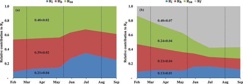
R. Qubaja et al.: Partitioning of canopy and soil CO2 fluxes                                                                    701

less than in the surrounding shrub by ∼ 40 % (Gelfand et al.,        and βw = 1.34+0.46 exp(−0.5((DoY−162)/66.1)2 ), where
2012).                                                               DoY is the day of the hydrological year starting from 1 Oc-
   The soil at the research site is shallow (20–40 cm), reach-       tober. Finally, GPP was calculated as GPP = NEE–Re . Neg-
ing only 0.7–1.0 m; the stoniness fraction for the soil depth        ative values of NEE and GPP indicated that the ecosystem
(0–1.2 m) is 15 %–60 %, and the rock cover of the surface            was a CO2 sink.
ranges between 9 % and 37 %, as recently described in de-               Half-hourly auxiliary measurements used in this study in-
tail (Preisler et al., 2019); the soil is eolian-origin loess with   cluded photosynthetic activity radiation (PAR; mol m−2 s−1 ),
a clay–loam texture (31 % sand, 41 % silt, and 28 % clay;            vapor pressure deficit (VPD; kPa), wind speed (m s−1 ), and
density is 1.65 ± 0.14 g cm−3 ) overlying chalk and limestone        relative humidity (RH; %), with additional measurements as
bedrock. Deeper soils (up to 1.5 m) are sporadically located         described elsewhere (Tatarinov et al., 2016). Furthermore,
at topographic hollows. While the natural rocky hill slopes          the soil microclimatology half-hourly measurements were
in the region are known to create flash floods, the forested         measured and calculated with soil chamber measurements,
plantation reduces runoff dramatically to less than 5 % of an-       using the LI-8150-203 (LI-COR, Lincoln, NE), as described
nual rainfall (Shachnovich et al., 2008). Groundwater is deep        below, namely air temperature (Ta ; ◦ C) and relative humid-
(> 300 m), reducing the possibility of groundwater recharge          ity at 20 cm above the soil surface and soil temperature (Ts ;
due to negative hydraulic conductivity or of water uptake by         ◦ C) at a 5 cm soil depth using a soil temperature probe, as

trees from the groundwater.                                          well as volumetric soil water content (SWC0−10 ; m3 m−3 )
                                                                     in the upper 10 cm of the soil near the chambers, using the
2.2   Flux and meteorological measurements                           ThetaProbe model ML2x (Delta-T Devices Ltd., Cambridge,
                                                                     UK), which was calibrated to the soil composition based on
An instrumented eddy covariance (EC) tower was erected in            the manufacturer’s equations.
the geographical center of Yatir Forest, following the EU-
ROFLUX methodology (Aubinet et al., 2000). The system                2.3    Soil CO2 fluxes
uses a three-dimensional (3-D) sonic anemometer (Omnidi-
rectional R3, Gill Instruments, Lymington, UK) and a closed          Soil CO2 fluxes (Rs ) were measured with automated non-
path LI-7000 CO2 /H2 O gas analyzer (LI-COR Inc., Lincoln,           steady-state systems, using 20 cm diameter opaque cham-
NE, USA) to measure the evapotranspiration flux (ET) and             bers and a multiplexer to allow for simultaneous control of
net CO2 flux (NEE). EC flux measurements were used to                several chambers (LI-8150, -8100-101, -8100-104; LI-COR,
estimate the annual scale of NEP by integrating half-hourly          Lincoln, NE). The precision of CO2 measurements in the
NEE values. The long-term operation of our EC measure-               chambers’ air is ±1.5 % of the measurements’ range (0–
ment site (since 2000; see Rotenberg and Yakir, 2010) pro-           20 000 ppm). The chambers were closed on preinstalled PVC
vides continuous flux and meteorological data with about             collars of 20 cm diameter, allowing for a short measurement
80 % coverage, which are subjected to U∗ nighttime correc-           time (i.e., 2 min), and positioned away from the collars for
tion and quality control, and gap filling is based on the extent     the rest of the time. Data were collected using a system in
of the missing data, as recently described in more detail in         which air from the chambers was circulated (2.5 L min−1 )
Tatarinov et al. (2016). A site-specific algorithm was used          through an infrared gas analyzer (IRGA) to record CO2
for flux partitioning into Re and GPP. Daytime ecosystem             (µmol CO2 mol−1 air) and H2 O (mmol H2 O mol−1 air) con-
respiration (Re − d; in µmol m−2 s−1 ) was estimated based           centrations in the system logger (1 s−1 ). Gap filling of miss-
on measured nighttime values (Re − n; i.e., when the global          ing data due to technical problems (i.e., 27 % of the data
radiation was < 5 W m−2 ), averaged for the first 3 half hours       across the study period between November 2015 and Octo-
of each night. The daytime respiration for each half hour was        ber 2016) was based on the average diurnal cycle of each
calculated according to Eq. (3) (Maseyk et al., 2008a; Tatari-       month.
nov et al., 2016):                                                      The rates of soil CO2 flux, Rs (µmol CO2 m−2 s−1 ), were
                                                                   calculated from chamber data using a linear fit of change in
Re−d = Re−n α1 βsdTs + α2 βwdTa + α3 βfdTa ,                 (3)     the water-corrected CO2 mole fraction using Eq. (4) as fol-
where βs , βw , and βf are coefficients that correspond to soil,     lows:
wood, and foliage, respectively; dTs and dTa are soil and air               dC v P
temperature deviations from the values at the beginning of           Rs =     ·       ,                                         (4)
                                                                            dt s Ta R
the night; and α1, α2, and α3 are partitioning coefficients
fixed at 0.5, 0.1, and 0.4, respectively. The βs , βw , and βf co-   where dC/dt is the rate of change in the water-corrected
efficients were calculated as follows: βs values were based on       CO2 mol fraction (µmol CO2 mol−1 air s−1 ), v is the system
Q10 from the Grünzweig et al. (2009) study at the same site,         volume (m3 ), P is the chamber pressure (Pa), s is the soil
where βs = 2.45 for wet soil (i.e., SWC in the upper 30 cm           surface area within the collar (m2 ), Ta is the chamber air
above 20 % vol.); βs = 1.18 for dry soil (i.e., SWC in the up-       temperature (K), and R is the gas constant (J mol−1 K−1 ).
per 30 cm equal to or below 20 % vol.); βf = 3.15–0.036 Ta ;         A measurement period of 2 min was used, based on prelim-

www.biogeosciences.net/17/699/2020/                                                           Biogeosciences, 17, 699–714, 2020
702 R. Qubaja et al.: Partitioning of canopy and soil CO2 fluxes
inary tests to obtain the most linear increase of CO2 in the 114 C isotope signatures of monthly Rs locate it inside the
chambers with the highest R 2 . triangle (Fig. S2):
Soil CO2 fluxes in the experimental plot were measured
between November 2015 and October 2016 by means of δ 13 CRs = fsa · δ 13 Csa + fh · δ 13 Ch + fi · δ 13 Ci , (9)
three measurement chambers using 21 collars grouped in 14 14 14 14
1 CRs = fsa · 1 Csa + fh · 1 Ch + fi · 1 Ci , (10)
seven sites in the forest stand, with three locations (i.e., three 1 = fsa + fh + fi , (11)
collars) per site, based on different distances from the nearest
tree (Dt ). The collars were inserted 5 cm into the soil. Data where f indicates the fraction of total soil flux (e.g.,
were recorded on a half-hourly basis (48 daily records). The fh = Rh /Rs ), while subscripts sa, h, and i indicate au-
three chambers were rotated between the seven sites every 1– totrophic, heterotrophic, and inorganic components,
2 weeks to cover all sites and to assess spatial and temporal respectively. The three-equations system was used
variations. to solve the three unknown f fractions of the total
Upscaling of the collar measurements to plot-scale soil soil flux based on empirical estimates of the isotopic
CO2 flux was carried out by grouping collars based on three end-members. Additionally, δ 13 C and 114 C are the
locations (i.e., under trees (< 1 m from nearest tree; UT), in stable and radioactive carbon isotopic ratios, where
gaps between trees (1–2.3 m; BT), and in open areas (> 2.3 m; δ 13 C = [([13 C/12 C]sample / [13 C/12 C]reference ) −1] ·1000 ‰,
OA)), with one chamber taking measurements at each loca- and the reference is the Vienna international standard
tion, and estimating the fractional areas (∅) of the three lo- (VPDB). Radiocarbon data are expressed as 114 C
cations based on mapping the sites according to the distances in parts per thousand or per mil (‰), which is the
noted above, as previously done by Raz-Yaseef et al. (2010): deviation of a sample 14 C /12 C ratio relative to the
OxI standard in 1950 (see Taylor et al., 2015), that
Rs = RsOA · ∅OA + RsBT · ∅BT + RsUT · ∅UT , (5) is, 114 C = [([14 C/12 C]sample / (0.95· [14 C/12 C]reference ·
∅OA + ∅BT + ∅UT = 1. (6) exp [(y − 1950)/8267])) −1] ·1000 ‰, where y is the year
of sample measurements.
The annual scale of Rs was derived from the upscaled cham- The δ 13 CRs was estimated monthly using the Keeling plot
ber measurements (Eq. 5) based on daily records (48 half- approach (Figs. S3 and S4; Pataki et al., 2003; Taneva and
hourly values) of spatially upscaled Rs . Gonzalez-Meler, 2011). Soil air was sampled using closed-
Estimating the temperature sensitivity of Rs (Q10 ) was end stainless-steel tubes (6 mm diameter) perforated near the
performed as described by Davidson and Janssens (2006) tube bottom at four depths (30, 60, 90, and 120 cm). Sam-
using a first-order exponential equation (see also Xu et al., ples of soil air were collected in pre-evacuated 150 mL glass
2015): flasks with high-vacuum valves, the dead volume in the tub-
ing and flask necks having been purged with soil air using a
Rs = a e b T s , (7) plastic syringe equipped with a three-way valve.
Note that the Keeling plot approach is based on the two-
where Rs represents the half-hourly spatially upscaled time
end-member mixing model (see Review of Pataki et al.,
series of soil respiration flux (µmol m−2 s−1 ), Ts (◦ C) is soil
2003), which often does not hold in soils because of varia-
temperature at a 5 cm depth (upscaled spatially and tempo-
tions in the δ 13 C values of source material with depth (see
rally using the same method as for Rs ), and a and b are fit-
a recent example in Joseph et al., 2019). However, prob-
ted parameters. The b values were used to calculate the Q10
ably because of the very dry conditions at our study site,
value according to the following equation:
no change in δ 13 C with depths in the root zone is observed
Q10 = e10b . (8) (±0.1 ‰ across the 35 cm depth profiles; Fig. S5), provid-
ing an opportunity to avoid this caveat; we must also con-
2.4 Soil CO2 flux partitioning clude of course that the variations among the contributions
of Rsa , Rh , and Ri do not change significantly with depth,
The determination of different sources of soil CO2 efflux permitting the use of the single set of isotopic signatures in
was based on linear mixing models (Lin et al., 1999) to es- Table 2. The soil CO2 samplings carried out therefore repre-
timate proportions of three main sources (autotrophic, het- sented predominantly the mixing of atmospheric CO2 with a
erotrophic, and abiotic), using isotopic analysis of soil CO2 single integrated soil source signal, consistent with the Keel-
profiles and soil incubation data from eight campaigns (Jan- ing plot approach.
uary to September) during 2016, according to Eqs. (9)–(11). The autotrophic (δ 13 Csa ) end-member was estimated
Partitioning of the monthly Rs values into components was based on incubations during the sampling periods of ex-
done using a three-end-member triangular model for inter- cised roots, following Carbone et al. (2008). Fine roots
preting the δ 13 C and 114 C values of CO2 flux; the three- (< 2 mm diameter) were collected, rinsed with deionized wa-
end-member triangular corners are the autotrophic (Rsa ), het- ter, and incubated for 3 h in 10 mL glass flasks connected
erotrophic (Rh ), and abiotic (Ri ) sources of Rs . The δ 13 C and with Swagelok Ultra-Torr tee fittings to 330 mL glass flasks
Biogeosciences, 17, 699–714, 2020 www.biogeosciences.net/17/699/2020/R. Qubaja et al.: Partitioning of canopy and soil CO2 fluxes 703
equipped with Louwers high-vacuum valves. The flasks were δ 13 C analyses and four standards per 10 samples for [CO2 ]
flushed with CO2 -free air at room temperature close to field analyses.
conditions. The CO2 was allowed to accumulate to at least Organic matter samples were dried at 60 ◦ C and milled us-
2000 ppm (∼ 2 h). ing a Wiley mill fitted with a size 40 mesh, and soil samples
The heterotrophic (δ 13 Ch ) end-member was estimated as were ground in a pestle and mortar. Soils containing carbon-
in Taylor et al. (2015), and, similar to the root-incubation ex- ates were treated with 1 M hydrochloric acid. Between 0.2
periment, soil samples from the top 5 cm of the litter layer and 0.4 mg of each dry sample was weighed into tin cap-
or 10 cm below the soil surface were collected, and roots sules (Elemental Microanalysis Ltd., Okehampton, UK), and
were carefully removed to isolate heterotrophic components. the δ 13 C of each was determined using an elemental an-
Root-free soils were placed in 10 mL glass flasks and al- alyzer linked to a Micromass Optima IRMS (Manchester,
lowed to incubate for 24 h before being transferred to evacu- UK). Three replicates of each sample were analyzed, and
ated 330 mL glass flasks. The inorganic source (δ 13 Ci ) end- two samples of a laboratory working standard cellulose were
member was estimated using 1 g of dry soil (ground to pass measured for every 12 samples. Four samples of the ac-
through a 0.5 mm mesh) placed in a 10 mL tube with a sep- etanilide (Elemental Microanalysis Ltd.) international stan-
tum cap; then, 12 mL of 1 M HCl was added to dissolve the dard were used to calibrate each run, and a correction was
carbonate fraction, and the fumigated CO2 withdrawn from applied to account for the influence of a blank cup. The pre-
each tube was collected using a 10 mL syringe and injected cision was 0.1 ‰.
into a 330 mL evacuated flask for isotopic analysis.
Radiocarbon estimates were based on the work of Carmi 2.6 Total belowground carbon allocation (TBCA)
et al. (2013) at the same site, adjusted to the measured atmo-
spheric 14 C values during the study period (49.5 ‰; Carmi TBCA (g C m−2 yr−1 ) was calculated following Giardina
et al., 2013). The 114 Csa and 114 Ch end-members were es- and Ryan (2002) for the study year (November 2015–
timated based on the assumption that they carry the 14 C sig- October 2016) as follows:
natures of 4 and 8.5 years, respectively, older than the 14 C
TBCA = Rs − Ralp + 1Csoil , (12)
signature of the atmosphere at the time of sampling, based on
mean ages previously estimated (Graven et al., 2012; Levin et where Ralp is the annual aboveground litter production be-
al., 2010; Taylor et al., 2015). The ratio 114 Ci was obtained tween November 2014 and October 2015, and 1Csoil is the
from Carmi et al. (2013). Monthly values of 114 CRs were annual change in belowground total soil organic C. Litter
obtained using the linear equation of the regression line of production, not measured during the present study, was es-
the measured δ 13 C values of Rsa , Rsh, and Ri and the corre- timated based on values obtained by Masyk et al. (2008) for
sponding estimated 114 C values (Fig. S2) and monthly δ 13 C 2000–2006 (56 g C m−2 yr−1 ) and assumed to have increased
values of Rs . in the study period (2014–2015) proportionally to the mea-
sured increase in leaf area index (LAI; 1.31 to 1.94; i.e.,
2.5 Isotopic analysis Ralp = [(1.94·56)/1.31] = 83 g C m−2 yr−1 ). For herbaceous
litter production, three plots of 25 m2 were randomly selected
Isotopic analysis followed the methodology described in in 2002 and harvested at the end of the growing season, to-
Hemming et al. (2005). The δ 13 C of CO2 in the air was tal fresh biomass was weighed, and subsamples were used to
analyzed using a continuous-flow mass spectrometer con- determine dry weight and C content. Grünzweig et al. (2007)
nected to a 15-flask automatic manifold system. An aliquot of found that herbaceous litter production was close to the av-
1.5 mL of air was expanded from each flask into a sampling erage rainfall for the specific year; this method was adapted
loop on a 15-position valve (Valco, Houston, TX, USA). CO2 in the current study for the period between November 2014
was cryogenically trapped from the air samples using he- and October 2015. Since aboveground litter (Ralp ; the sum
lium as a carrier gas; it was then separated from N2 O with of tree litter and herbaceous litter production) of a given year
a Carbosieve G (Sigma-Aldrich) packed column at 70 ◦ C was mainly produced during that year but decayed during
and analyzed on a Europa 20-20 isotope ratio mass spec- the following hydrological year, TBCA was based on the
trometer (IRMS; Sercon, Crewe, UK). The δ 13 C results were current year’s Rs (2015–2016) and the previous year’s Ralp
quoted in parts per thousand (‰) relative to the VPDB in- (2014–2015). 1Csoil was set constant as the average annual
ternational standard. The analytical precision was 0.1 ‰. To belowground carbon increase since afforestation (Qubaja et
measure [CO2 ], an additional 40.0 mL subsample of air from al., 2019).
each flask was expanded into mechanical bellows and then
passed through an infrared gas analyzer (LI-6262; LI-COR, 2.7 Statistical analyses
Lincoln, NE, USA) in an automated system. The precision
of these measurements was 0.1 ppm. Flasks filled with cali- Two-way ANOVA tests were performed at a significance
brated standard air were measured with each batch of 10 sam- level set at p = 0.001 to detect significant effects of loca-
ple flasks; five standards were measured per 10 samples for tions (OA, BT, and UT), sites, and their interactions on Rs
www.biogeosciences.net/17/699/2020/ Biogeosciences, 17, 699–714, 2020704 R. Qubaja et al.: Partitioning of canopy and soil CO2 fluxes
and metrological parameters. Pearson correlation analysis (r) ing sharp differences between the wet and dry seasons. As
was used to detect the correlation between Rs and mete- previously observed in this semiarid site, all CO2 fluxes peak
orological parameters. To quantify spatiotemporal variabil- in early spring between March and April. The correspond-
ity in Rs , the coefficient of variation (CV %) was calculated ing high-resolution data are reported in Fig. S6, which show
as [(STDEV / Mean) · 100 %]. Heterogeneity was considered also that the high winter (February) Rs rates were associ-
weak if CV % ≤ 10 %, moderate if 10 % < CV % ≤ 100 %, ated with clear days when photosynthetic active radiation
and strong if CV % > 100 %. All the analyses were per- (PAR) increased with air temperature, Ta . These data also
formed using MATLAB software, Version R2017b (Math- show that, following rainy days, daily Rs values could reach
Works, Inc., MA, USA). 6.1 µmol m−2 s−1 (i.e., in the UT microsite; data not shown),
although the average was 1.1 ± 0.2 µmol m−2 s−1 during the
wet period, which diminished by ∼ 55 % in the dry season
3 Results to mean daily values of 0.5 ± 0.1 µmol m−2 s−1 . In spring
(April), all CO2 fluxes peaked during the crossover trends of
3.1 Spatial variations
decreasing soil moisture content and increasing temperature
The spatial variations in Rs across locations (distance from and PAR (Fig. S6).
nearest tree) and sites (across the study area) are re- The temporal variations in the half-hourly values of Rs re-
ported in Table 1, together with other measured variables. flected changes in soil moisture at 0–5 cm depth and PAR
The results indicated an overall mean Rs value of 0.8 ± (r = 0.5 and 0.2, respectively; pR. Qubaja et al.: Partitioning of canopy and soil CO2 fluxes 705
Table 1. Annual mean of half-hourly values across locations (OA, open area; BT, between trees; UT, under tree) in seven sites in the forest
during the study period of soil respiration flux rates (Rs ) together with the soil water content at 10 cm depth (SWC), minimum distances
from nearby tree (Dt ), soil temperature at 5 cm depth (Ts ), and air temperature (Ta ) and relative humidity (RH) at the soil surface (numbers
in parentheses indicate ±SE).
Locations Sites Rs SWC Dt Ts Ta RH
(µmol m−2 s−1 ) (×100 m3 m−3 ) (m) (◦ C) (◦ C) (%)
OA 1 1.64 (0.02) 16.5 (0.2) 2.9 15.6 (0.1) 15.4 (0.2) 59.7 (0.5)
2 0.72 (0.01) 14.5 (0.2) 3.6 15.9 (0.2) 15.0 (0.2) 58.4 (0.6)
3 1.23 (0.02) 19.3 (0.2) 7.0 20.6 (0.3) 18.2 (0.2) 53.5 (0.5)
4 0.38 (0.01) 11.3 (0.2) 3.0 22.6 (0.2) 20.8 (0.1) 58.9 (0.4)
5 0.38 (0.01) 5.8 (0.2) 3.0 25.5 (0.1) 24.0 (0.1) 43.1 (0.4)
6 0.31 (0.01) 5.7 (0.4) 2.8 30.0 (0.3) 26.2 (0.3) 51.8 (0.9)
7 0.14 (0.01) 6.1 (0.3) 3.5 25.5 (0.2) 23.2 (0.3) 44.5 (0.9)
Average 0.68 (0.21) 11 (0) 3.7 (0.6) 22.3 (2.0) 20.4 (1.6) 52.8 (2.6)
CV (%) 81 % 50 % 41 % 13 %
BT 1 0.77 (0.01) 10.5 (0.2) 1.8 16.1 (0.1) 15.2 (0.2) 60.5 (0.5)
2 0.88 (0.01) 12.1 (0.2) 1.5 14.8 (0.2) 14.7 (0.2) 59.5 (0.6)
3 0.84 (0.01) 20.4 (0.2) 2.7 20.1 (0.3) 18.4 (0.2) 54.1 (0.6)
4 0.91 (0.01) 14.4 (0.2) 2.7 23.3 (0.2) 21.3 (0.2) 58.5 (0.4)
5 0.41 (0.00) 3.9 (0.2) 2.0 24.6 (0.1) 24.0 (0.1) 43.2 (0.4)
6 0.41 (0.01) 3.3 (0.4) 2.5 29.1 (0.2) 26.0 (0.3) 52.5 (0.8)
7 0.46 (0.01) 5.5 (0.3) 1.2 23.9 (0.1) 22.8 (0.3) 45.7 (0.9)
Average 0.67 (0.09) 10 (0) 2.0 (0.2) 21.7 (1.9) 20.3 (1.6) 53.4 (2.6)
CV (%) 35 % 63 % 29 % 13 %
UT 1 1.22 (0.02) 9.3 (0.2) 0.2 15.7 (0.1) 15.2 (0.2) 60.0 (0.5)
2 1.42 (0.01) 14.0 (0.2) 0.3 14.8 (0.2) 14.8 (0.2) 59.4 (0.6)
3 1.64 (0.01) 19.8 (0.2) 0.5 19.0 (0.2) 18.0 (0.2) 54.5 (0.6)
4 1.90 (0.02) 11.3 (0.2) 0.6 22.0 (0.1) 20.8 (0.1) 59.0 (0.4)
5 1.16 (0.01) 4.0 (0.2) 0.4 23.9 (0.1) 23.7 (0.1) 44.1 (0.4)
6 1.29 (0.01) 4.5 (0.4) 0.2 29.5 (0.3) 25.9 (0.3) 52.7 (0.9)
7 0.89 (0.01) 5.2 (0.3) 0.2 25.0 (0.1) 23.0 (0.3) 45.5 (0.9)
Average 1.36 (0.13) 10 (0) 0.3 (0.1) 21.4 (2.0) 20.2 (1.6) 53.6 (2.5)
CV (%) 25 % 60 % 46 % 12 %
All Average (SE) 0.8 (0.1) 11 (0) 2.0 (0.4) 21.8 (1.1) 20.3 (0.9) 53.3 (1.4)
Max 1.90 20 7.0 30.0 26.2 60.5
Min 0.14 3 0.2 14.8 14.7 43.1
CV (%) 55 % 55 % 82 % 12 %
Two-way Site 0.000 0.000 0.000 0.000 0.000
ANOVA Location 0.000 0.000 0.000 0.220 0.074
(P value) Site × location 0.000 0.000 0.000 0.645 0.961
Pearson Correlation with Rs 0.50∗ −0.62∗∗ −0.45∗ −0.45∗ 0.50∗
∗ Correlation is significant at the 0.05 level (two-tailed). ∗∗ Correlation is significant at the 0.01 level (two-tailed).
fraction – the fraction of inorganic sources from the total soil Rs /Re from 75 % to 46 % on average from the wet to the dry
respiration – ranged from 0.09 to 0.35, the largest contribu- season, respectively, which reflected a seasonal change of Rf
tion being in the driest period. The mean relative contribu- in the wet season to peak values in the dry season (Fig. 3b).
tions of these components to Rs over the sampling campaigns Both the highest and lowest Rs fractions (∼ 0.74 and nearly
are presented in Fig. 3a, but, on average, soil biotic fluxes 0.34) along the seasonal cycle were associated with low total
were higher than abiotic fluxes by a factor of ∼ 4. Re parti- Re fluxes, that is, in the fall before the Rf peak in the spring
tioning showed an average increase in Rf /Re from 25 % in and in the summer, when physiological controls limited wa-
the wet season to 54 % in the dry season and a decline in ter loss (Fig. 2).
www.biogeosciences.net/17/699/2020/ Biogeosciences, 17, 699–714, 2020706 R. Qubaja et al.: Partitioning of canopy and soil CO2 fluxes
Figure 1. Representative diurnal cycles of soil respiration (Rs ; using soil chambers across locations: open area, OA; between trees, BT; under
trees, UT) and sites in panels (a) and (b), of net ecosystem exchange (NEE; canopy-scale eddy covariance) and gross primary production
(GPP) and ecosystem respiration (Re ) and its partitioning to soil respiration (Rs ) and aboveground tree respiration (Rf ) in panels (c) and (d),
during the wet (November–April) and dry (May–October) periods. Based on half-hourly values over the diurnal cycle; shaded areas indicate
±SE; Rf was estimated as the residual as Rf = Re − Rs and is presented as a dashed line.
Table 2. The δ 13 C and 114 C signature of soil respiration (Rs ) and its partitioning into autotrophic (Rsa ), heterotrophic (Rh ), and abiotic (Ri ),
together with the relative contribution of each to the soil and ecosystem respiration for Yatir Forest during eight campaigns of measurements
from January to September 2016 (numbers in parentheses indicate ±SE) in comparison to results obtained previously in the same forest
(2001–2006 mean values). The monthly contribution of Rsa , Rh , and Ri to Rs or Re is presented in Fig. 3a and b, respectively.
Signature Rsa Rh Ri Rs
(‰)
δ 13 C −23.7 (0.5)1 −24.3 (0.0)1 −6.5 (0.0)1 −20.8 (±0.6)1
114 C 303 503 −9002 −134 (34)4
Relative contribution 0.40 (0.02) 0.39 (0.02) 0.21 (0.04)
to Rs (2015–2016)
Relative contribution 0.24 (0.04) 0.23 (0.04) 0.13 (0.01) 0.60 (0.06)
to Re (2015–2016)
1 Measured in the present study. 2 Measured by Carmi et al. (2013). 3 Calculated based on the measured
atmospheric value by Carmi et al. (2013). 4 Calculated based on the best-fit regression equation in Fig. S2.
Biogeosciences, 17, 699–714, 2020 www.biogeosciences.net/17/699/2020/R. Qubaja et al.: Partitioning of canopy and soil CO2 fluxes 707
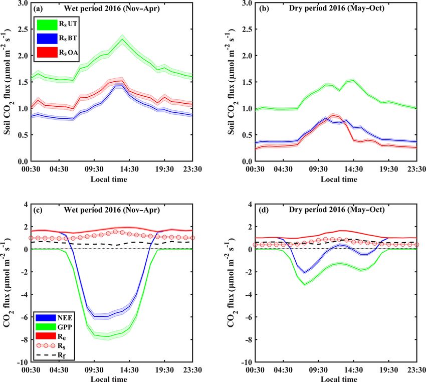
Figure 2. Seasonal trends of monthly mean values during the research period of (a) the fluxes of net ecosystem exchange (NEE), gross pri-
mary production (GPP), and ecosystem respiration (Re ) and its components, soil respiration (Rs ) and aboveground tree respiration (Rf ), and
monthly mean of precipitation (P), and monthly mean of key environmental parameters; (b) soil water content at the top 10 cm (SWC0−10 )
and soil temperature at 5 cm (Ts ); and (c) vapor pressure deficit (VPD) and photosynthetic activity radiation (PAR). Rf is obtained from
Re -Rs . Vertical dotted lines indicate the winter, spring, summer, and fall seasons.
3.3 Annual scale making up 60 ± 6 % of Re (295 ± 4 g C m−2 yr−1 ; Tables 3
and S1), and Rf was another significant component account-
ing for 40 ± 6 % of Re (Fig. 3b), which reflected the low-
On an annual timescale, estimates of CO2 flux components
density (300 trees ha−1 ) nature of the semiarid forest. As in-
based on EC measurements resulted in annual values of GPP,
dicated above, Re partitioning showed a decrease in Rs /Re
NPP, Re , and NEP of 655, 282, 488, and 167 g C m−2 yr−1 ,
and an increase in Rf /Re from winter to summer, which is
respectively (Tables 3 and S1). On average across the mea-
clearly apparent in Fig. 3b. On an annual scale, during the
surement period, Rs was the main CO2 flux to atmosphere,
www.biogeosciences.net/17/699/2020/ Biogeosciences, 17, 699–714, 2020708 R. Qubaja et al.: Partitioning of canopy and soil CO2 fluxes
Figure 3. (a) Seasonal variations in the relative contribution of soil autotrophic (Rsa ), heterotrophic (Rh ), and abiotic (Ri ) components to
Rs , and (b) seasonal variations in the relative contribution of soil autotrophic (Rsa ), heterotrophic (Rh ), abiotic (Ri ), and foliage and stem
respiration (Rf is obtained from Re − Rs ) components to ecosystem respiration (Re ) during eight campaigns (January–September) in 2016.
The contributions were estimated with linear mixing models using δ 13 C and 114 C of soil respiration (Rs ) and a soil CO2 profile method at
0 to 120 cm soil depth. Vertical dotted lines indicate the winter, spring, summer, and fall seasons. These results confirmed earlier estimates
of Grünzweig et al. (2009) and Maseyk et al. (2008a).
Table 3. Mean annual values of ecosystem respiration (Re ), its components and associated ratios, net ecosystem exchange (NEE; from eddy
covariance), net primary productivity (NPP), gross primary productivity (GPP), carbon-use efficiency (CUE), leaf area index (LAI), and
ratio of total belowground carbon allocation (TBCA) to GPP (TBCA / GPP) in the present study (mean of November 2015 to October 2016)
and in comparison to results obtained previously in the same forest (2001–2006 mean values). Ri , Rh , Rsa , Rs , Rl and Rw denote abiotic,
heterotrophic, soil autotrophic, soil, foliage, and wood CO2 flux, respectively. Q10 is derived during the two studies for the wet and dry
seasons.
Study Rs Rh Rsa Rl Rw Ri Re NEE NPP GPP
(g m−2 yr−1 )
Mean (2001–2006) 406 147 203 260 70 56 735 −211 −358 −880
x/Rs 0.36 0.50 0.14
x/Re 0.55 0.20 0.28 0.35 0.10 0.07
Mean (2015–2016) 295 115 119 155 39 61 488 −167 −282 −655
x/Rs 0.39 0.40 0.21
x/Re 0.60 0.23 0.24 0.32 0.08 0.13
Ratio of (x/Rs )2016 /(x/Rs )2003 1.08 0.81 1.50
Ratio of (x/Re )2016 /(x/Re )2003 1.09 1.18 0.88 0.90 0.84 1.64
Study Q10 CUE TBCA / GPP3 LAI
SWC1 SWC2 (m2 m−2 )
Mean (2001–2006) 2.5 1.2 0.40 0.41 1.3
Mean (2015–2016) 1.6 1.1 0.43 0.38 2.1
Ratio of x2016 /x2003 0.64 0.92 1.06 0.93 1.62
1 SWC ≥ 0.2 (m3 m−3 ). 2 SWC < 0.2 [m3 m−3 ]. 3 The mean of GPP used by Grünzweig et al. (2009) to estimate the TBCA / GPP ratio was
834 g m−2 yr−1 .
Biogeosciences, 17, 699–714, 2020 www.biogeosciences.net/17/699/2020/R. Qubaja et al.: Partitioning of canopy and soil CO2 fluxes 709
study period, estimates of Rf , Rsa , Rh , and Ri values were Carbon partitioning belowground (TBCA / GPP) was rela-
194 ± 36, 119 ± 21, 115 ± 20, and 61 ± 6 g C m−2 yr−1 , re- tively high (∼ 38 %), with little change across the long-term
spectively. These rates of respiration fluxes translated at the observation period. It is, however, within the range of mean
ecosystem scale to Re / GPP of ∼ 75 %, lower than observed values for forests in different biomes (Litton et al., 2007).
in other ecosystems (Table S3) and leading, in turn, to high High belowground allocation helps explain the high rate of
ecosystem CUE of 0.43. SOC (soil organic carbon) accumulation observed over the
Using the site records of nearly 20 years, long-term trends period since afforestation (Grünzweig et al., 2007; Qubaja
in GPP, NPP, Re , and NEP were examined. Soil respiration et al., 2019). Note that, irrespective of the soil carbon accu-
and its partitioning could not be similarly monitored con- mulation, the abiotic component to the CO2 flux seems to
tinuously, but combining the present results with the 2001– be significant in dry environments (Table 3) and in particular
2006 values obtained by Grünzweig et al. (2009) and Maseyk in the dry seasons, when biological activities drastically de-
et al. (2008a) provided a basis for estimating the long-term crease (Kowalski et al., 2008; Lopez-Ballesteros et al., 2017;
trends in soil respiration. Notably, no clear or significant Serrano-Ortiz et al., 2010; Martí-Roura et al., 2019). The re-
trend over time was observed in any of the canopy-scale con- sults show that considering the abiotic effects on estimating
tinuously monitored fluxes, but, because of relatively large soil respiration and, in turn, on estimating the carbon budget
interannual variations, associated mainly with those in pre- in dry calcareous soils can play an important part in estimat-
cipitation (see Qubaja et al., 2020), it is likely that the rela- ing soil and ecosystem respiration fluxes (Angert et al., 2015;
tive contributions of the different fluxes, expressed as ratios Roland et al., 2012).
in Table 3, provide a more robust perspective of the long-term The soil CO2 efflux in the semiarid forest
temporal changes in the ecosystem functioning. The results (295 g C m−2 yr−1 ) is at the low end of Rs values across
presented in Table 3 reflect the long-term growth of the for- the range of climatic regions, from 50 to 2750 g C m−2 yr−1
est, with a relatively large increase in LAI, but the TBCA re- (Adachi et al., 2017; Chen et al., 2014; Grünzweig et al.,
mained around 40 %. The results also indicated little change 2009; Hashimoto et al., 2015). This is clearly lower than the
in the total soil respiration, Rs , component, (as a fraction of mean Rs value for global evergreen needle forests, which
Re or GPP) but a general shift from the autotrophic com- is estimated at 690 g C m−2 yr−1 (Chen et al., 2014), and
ponents to the heterotrophic component (i.e., Rh ). This was between estimates for desert scrub and Mediterranean wood-
reflected in the decreasing ratio of the autotrophic compo- land (224–713 g C m−2 yr−1 ; Raich and Schlesinger, 1992)
nents (i.e., Rsa , Rl , and Rw ) and the increasing ratio of Rh to or for Mediterranean forests (561–1,015 g C m−2 yr−1 ;
Re (Table 3) across the 13-year observation period (2003 to Casals et al., 2011; Luyssaert et al., 2007; Matteucci et al.,
2016). 2015; Misson et al., 2010; Rey et al., 2002; Rodeghiero
and Cescatti, 2005). The mean instantaneous rate of Rs ,
0.8 µmol m−2 s−1 , is also in the range reported for unman-
4 Discussion aged forest and grassland in the dry Mediterranean region
(0.5 and 2.1 µmol m−2 s−1 ; Correia et al., 2012).
Partitioning ecosystem carbon fluxes and long-term obser-
The observed low Rs values were associated with a rel-
vational studies are key to understanding ecosystem carbon
atively high fraction of autotrophic and a lower fraction of
dynamics and their response to change. Overall, the results
heterotrophic respiration. The mean annual-scale Rsa /Rs ra-
support our research hypothesis that the observed high CUE
tio of 0.40 was at the high end of the global range of 0.09 to
at our site is at least partly due to the characteristics of the
0.49 (Chen et al., 2014; Hashimoto et al., 2015). In contrast,
carbon flux partitioning that can be associated with the semi-
heterotrophic respiration showed an annual-scale Rh /Rs ra-
arid conditions. Compared to other sites and climates (see
tio of 0.39 ± 0.02 (Table 2 and Fig. 3), which is lower than
comparative compilation in Table S3 in the Supplement), the
the estimated global mean Rh /Rs value of 0.56 (Hashimoto
results reflect several key points: (1) relatively high below-
et al., 2015) but within the range of Mediterranean region for-
ground allocation; (2) low soil respiration in general and low
est, which varies between 0.29 and 0.77 (Casals et al., 2011;
heterotrophic respiration in particular; (3) combining the re-
Luyssaert et al., 2007; Matteucci et al., 2015; Misson et al.,
sults for 2016 and those of our earlier study offered a long-
2010; Rey et al., 2002; Rodeghiero and Cescatti, 2005). The
term perspective across 13 years, indicating that the low Rs
relatively low annual scale of the heterotrophic respiration to
in this ecosystem is robust and exhibits reduced sensitivity to
Rs is consistent with the dry soil over much of the year in this
temperature; and (4) there is a general long-term shift from
forest (Figs. 2 and S6) and the observed low decomposability
autotrophic to heterotrophic respiration.
of plant detritus and the high mean SOC accumulation rate
Comparing CO2 fluxes in this forest with fluxes in a range
(Grünzweig et al., 2007).
of European forests showed that mean NEP in the semiarid
The long-term perspective from the 13-year observation
forest (167 g C m−2 yr−1 ) is similar to the mean NEP in other
period indicates emerging trends that can be a basis for as-
European forests (150 g C m−2 yr−1 ; FLUXNET).
sessing the effects of forest age and the evident increase in
LAI (Table 3) and changes in environmental conditions (gen-
www.biogeosciences.net/17/699/2020/ Biogeosciences, 17, 699–714, 2020710 R. Qubaja et al.: Partitioning of canopy and soil CO2 fluxes
erally warming and drying; see, e.g., Lelieveld et al., 2012). RQ and DY wrote the paper, with discussions and contributions to
Here, because comparing the noncontinuous data from the interpretations of the results from all the coauthors.
present (2016) and earlier (2001–2006) studies is sensitive
to the large interannual variations in the ecosystem activi-
ties and fluxes (Qubaja et al., 2019), we focused on the more Competing interests. The authors declare that they have no conflict
robust changes in the ratio of the respiration components to of interest.
the overall fluxes (Re ; Table 3). This shows a shifting trend
from the autotrophic components to the heterotrophic, with
little change in the contribution of Rs to the overall efflux. Acknowledgements. This long-term study was funded by the
Forestry Department of Keren Kayemeth LeIsrael (KKL) and the
The ratios of Rsa , Rl , and Rw to Re tended to decrease by
German Research Foundation (DFG) as part of the project “Cli-
about 13 %, while that of Rh increased by about 18 %; simi- mate feedbacks and benefits of semi-arid forests” (CliFF), by the Is-
lar trends were seen in soil respiration, with Rsa /Rs decreas- rael Science Foundation (ISF; grant no. 1976/17), and by the Israel
ing by −19 % and Rh /Rs increasing by +8 % (Table 3). The Science Foundation and the National Natural Science Foundation
relatively low Rs under conditions of high temperature in the of China (ISF–NSFC) joint research program (grant no. 2579/16).
semiarid ecosystem implies reduced sensitivity of respiration The authors thank Efrat Schwartz for assistance with lab work. The
to temperature. This is partly imposed by low SWC condi- long-term operation of the Yatir Forest Research Field Site is sup-
tions during extended parts of the year (Grünzweig et al., ported by the Cathy Wills and Robert Lewis Program in Environ-
2009; cf. Rey et al., 2002; Xu and Qi, 2001). Accordingly, mental Science. We thank the entire Yatir team for technical support
Rs showed greater sensitivity to Ts in the wet period, but, and the local KKL personnel for their cooperation.
during the 8–9 months of the year when SWC was below
∼ 0.2 m3 m−3 , Rs varied predominantly with water availabil-
ity. The long-term perspective reported in Table 3 indicates Financial support. This research has been supported by the
Forestry Department of Keren Kayemeth LeIsrael (KKL) and the
a further decrease in temperature sensitivity, with mean Q10
German Research Foundation (DFG) as part of the project “Climate
values in the dry season decreasing from 1.6 to 1.1. These feedbacks and benefits of semi-arid forests” (CliFF), the Israel Sci-
estimated Q10 values are generally consistent with published ence Foundation (ISF; grant no. 1976/17), and the National Natural
values for different ecosystems (1.4 to 2.0; Hashimoto et al., Science Foundation of China (ISF–NSFC) joint research program
2015; Zhou et al., 2009) and with low values under low SWC (grant no. 2579/16).
(Reichstein et al., 2003; Tang et al., 2005). This is also con-
sistent with soil warming experiments by 0.76 ◦ C in Mediter-
ranean ecosystems, which decreased the Rs by 16 % and Q10 Review statement. This paper was edited by Frank Hagedorn and
by 14 % (Wang et al., 2014). Note also that the low temper- reviewed by two anonymous referees.
ature sensitivity in the dry season is likely to be related to
reduced microbial activity but may also involve downregu-
lation of plant activity (Maseyk et al., 2008a) and drought-
induced dormancy of shallow roots (Schiller, 2000). Finally, References
we also note that the greater importance of moisture avail-
ability in influencing respiration is clearly apparent from the Adachi, M., Ito, A., Yonemura, S., and Takeuchi, W.: Estimation
of global soil respiration by accounting for land-use changes de-
observed relationships of Rs and Rh to mean annual precipi-
rived from remote sensing data, J. Environ. Manage., 200, 97–
tation (MAP) in European evergreen needle forests (Fig. S8;
104, https://doi.org/10.1016/j.jenvman.2017.05.076, 2017.
see also Grünzweig et al., 2007), which are not observed with Angert, A., Yakir, D., Rodeghiero, M., Preisler, Y., Davidson, E. A.,
respect to mean annual temperature. and Weiner, T.: Using O2 to study the relationships between soil
CO2 efflux and soil respiration, Biogeosciences, 12, 2089–2099,
https://doi.org/10.5194/bg-12-2089-2015, 2015.
Data availability. The data used in this study are archived Aubinet, M., Grelle, A., Ibrom, A., Rannik, U., Moncrieff, J., Fo-
and available from the corresponding author upon request ken, T., Kowalski, A. S., Martin, P. H., Berbigier, P., Bernhofer,
(dan.yakir@weizmann.ac.il). C., Clement, R., Elbers, J., Granier, A., Grunwald, T., Morgen-
stern, K., Pilegaard, K., Rebmann, C., Snijders, W., Valentini,
R., and Vesala, T.: Estimates of the annual net carbon and water
Supplement. The supplement related to this article is available on- exchange of forests: The EUROFLUX methodology, Adv. Ecol.
line at: https://doi.org/10.5194/bg-17-699-2020-supplement. Res., 30, 113–175, 2000.
Bahn, M., Janssens, I. A., Reichstein, M., Smith, P., and Trum-
bore, S. E.: Soil respiration across scales: towards an integra-
Author contributions. RQ and DY designed the study; RQ, FT, ER, tion of patterns and processes, New Phytol., 186, 292–296,
and DY performed the experiments. RQ and DY analyzed the data. https://doi.org/10.1111/j.1469-8137.2010.03237.x, 2010.
Balogh, J., Pinter, K., Foti, S., Cserhalmi, D., Papp, M., and
Nagy, Z.: Dependence of soil respiration on soil mois-
Biogeosciences, 17, 699–714, 2020 www.biogeosciences.net/17/699/2020/R. Qubaja et al.: Partitioning of canopy and soil CO2 fluxes 711 ture, clay content, soil organic matter, and CO2 uptake DeLucia, E. H., Drake, J. E., Thomas, R. B., and Gonzalez-Meler, in dry grasslands, Soil Biol. Biochem., 43, 1006–1013, M.: Forest carbon use efficiency: is respiration a constant frac- https://doi.org/10.1016/j.soilbio.2011.01.017, 2011. tion of gross primary production?, Glob. Change Biol., 13, 1157– Binkley, D., Stape, J. L., Takahashi, E. N., and Ryan, M. G.: 1167, https://doi.org/10.1111/j.1365-2486.2007.01365.x, 2007. Tree-girdling to separate root and heterotrophic respiration in Deng, Q., Hui, D., Zhang, D., Zhou, G., Liu, J., Liu, S., two Eucalyptus stands in Brazil, Oecologia, 148, 447–454, Chu, G., and Li, J.: Effects of Precipitation Increase https://doi.org/10.1007/s00442-006-0383-6, 2006. on Soil Respiration: A Three-Year Field Experiment Bonan, G. B.: Ecological climatology: concepts and applications, in Subtropical Forests in China, Plos One, 7, e41493, 2nd Edn., Cambridge: Cambridge University Press, Cambridge, https://doi.org/10.1371/journal.pone.0041493, 2012. 28–37, 2008. Etzold, S., Ruehr, N. K., Zweifel, R., Dobbertin, M., Zingg, A., Bond-Lamberty, B. and Thomson, A.: Temperature-associated in- Pluess, P., Hasler, R., Eugster, W., and Buchmann, N.: The Car- creases in the global soil respiration record, Nature, 464, 579– bon Balance of Two Contrasting Mountain Forest Ecosystems in 582, https://doi.org/10.1038/nature08930, 2010. Switzerland: Similar Annual Trends, but Seasonal Differences, Buchmann, N.: Biotic and abiotic factors controlling soil respiration Ecosystems, 14, 1289–1309, https://doi.org/10.1007/s10021- rates in Picea abies stands, Soil Biol. Biochem., 32, 1625–1635, 011-9481-3, 2011. https://doi.org/10.1016/s0038-0717(00)00077-8, 2000. Etzold, S., Zweifel, R., Ruehr, N. K., Eugster, W., and Buchmann, Carbone, M. S., Winston, G. C., and Trumbore, S. E.: Soil respi- N.: Long-term stem CO2 concentration measurements in Nor- ration in perennial grass and shrub ecosystems: Linking envi- way spruce in relation to biotic and abiotic factors, New Phytol., ronmental controls with plant and microbial sources on seasonal 197, 1173–1184, https://doi.org/10.1111/nph.12115, 2013. and diel timescales, J. Geophys. Res.-Biogeo., 113, G02022, Falge, E., Baldocchi, D., Tenhunen, J., Aubinet, M., Bakwin, P., https://doi.org/10.1029/2007jg000611, 2008. Berbigier, P., Bernhofer, C., Burba, G., Clement, R., Davis, K. Carmi, I., Yakir, D., Yechieli, Y., Kronfeld, J., and Stiller, M.: Vari- J., Elbers, J. A., Goldstein, A. H., Grelle, A., Granier, A., Guo- ations in soil CO2 concentrations and isotopic values in a semi- mundsson, J., Hollinger, D., Kowalski, A. S., Katul, G., Law, arid region due to biotic and abiotic processes in the unsaturated B. E., Malhi, Y., Meyers, T., Monson, R. K., Munger, J. W., zone, Radiocarbon, 55, 932–942, 2013. Oechel, W., Paw, K. T., Pilegaard, K., Rannik, U., Rebmann, C., Carvalhais, N., Forkel, M., Khomik, M., Bellarby, J., Jung, M., Suyker, A., Valentini, R., Wilson, K., and Wofsy, S.: Seasonality Migliavacca, M., Mu, M. Q., Saatchi, S., Santoro, M., Thurner, of ecosystem respiration and gross primary production as derived M., Weber, U., Ahrens, B., Beer, C., Cescatti, A., Randerson, from FLUXNET measurements, Agr. Forest Meteorol., 113, 53– J. T., and Reichstein, M.: Global covariation of carbon turnover 74, https://doi.org/10.1016/s0168-1923(02)00102-8, 2002. times with climate in terrestrial ecosystems, Nature, 514, 213– Flechard, C. R., Ibrom, A., Skiba, U. M., de Vries, W., van Oijen, 217, https://doi.org/10.1038/nature13731, 2014. M., Cameron, D. R., Dise, N. B., Korhonen, J. F. J., Buchmann, Casals, P., Lopez-Sangil, L., Carrara, A., Gimeno, C., and Nogues, N., Legout, A., Simpson, D., Sanz, M. J., Aubinet, M., Loustau, S.: Autotrophic and heterotrophic contributions to short-term soil D., Montagnani, L., Neirynck, J., Janssens, I. A., Pihlatie, M., CO2 efflux following simulated summer precipitation pulses in Kiese, R., Siemens, J., Francez, A.-J., Augustin, J., Varlagin, A., a Mediterranean dehesa, Global Biogeochem. Cy., 25, GB3012, Olejnik, J., Juszczak, R., Aurela, M., Chojnicki, B. H., Dämm- https://doi.org/10.1029/2010gb003973, 2011. gen, U., Djuricic, V., Drewer, J., Eugster, W., Fauvel, Y., Fowler, Chen, D., Zhang, Y., Lin, Y., Zhu, W., and Fu, S.: Changes in D., Frumau, A., Granier, A., Gross, P., Hamon, Y., Helfter, C., belowground carbon in Acacia crassicarpa and Eucalyptus uro- Hensen, A., Horváth, L., Kitzler, B., Kruijt, B., Kutsch, W. L., phylla plantations after tree girdling, Plant Soil, 326, 123–135, Lobo-do-Vale, R., Lohila, A., Longdoz, B., Marek, M. V., Mat- https://doi.org/10.1007/s11104-009-9986-0, 2010. teucci, G., Mitosinkova, M., Moreaux, V., Neftel, A., Ourcival, Chen, S. T., Zou, J. W., Hu, Z. H., Chen, H. S., and Lu, J.-M., Pilegaard, K., Pita, G., Sanz, F., Schjoerring, J. K., Se- Y. Y.: Global annual soil respiration in relation to cli- bastià, M.-T., Tang, Y. S., Uggerud, H., Urbaniak, M., van Dijk, mate, soil properties and vegetation characteristics: Sum- N., Vesala, T., Vidic, S., Vincke, C., Weidinger, T., Zechmeister- mary of available data, Agr. Forest Meteorol., 198, 335–346, Boltenstern, S., Butterbach-Bahl, K., Nemitz, E., and Sutton, https://doi.org/10.1016/j.agrformet.2014.08.020, 2014. M. A.: Carbon / nitrogen interactions in European forests and Conant, R. T., Klopatek, J. M., Malin, R. C., and Klopatek, semi-natural vegetation. Part I: Fluxes and budgets of carbon, C. C.: Carbon pools and fluxes along an environmental nitrogen and greenhouse gases from ecosystem monitoring and gradient in northern Arizona, Biogeochemistry, 43, 43–61, modelling, Biogeosciences Discuss., https://doi.org/10.5194/bg- https://doi.org/10.1023/a:1006004110637, 1998. 2019-333, in review, 2019a. Correia, A. C., Minunno, F., Caldeira, M. C., Banza, J., Mateus, Flechard, C. R., van Oijen, M., Cameron, D. R., de Vries, W., Ibrom, J., Carneiro, M., Wingate, L., Shvaleva, A., Ramos, A., Jongen, A., Buchmann, N., Dise, N. B., Janssens, I. A., Neirynck, J., M., Bugalho, M. N., Nogueira, C., Lecomte, X., and Pereira, Montagnani, L., Varlagin, A., Loustau, D., Legout, A., Ziem- J. S.: Soil water availability strongly modulates soil CO2 ef- blińska, K., Aubinet, M., Aurela, M., Chojnicki, B. H., Drewer, flux in different Mediterranean ecosystems: Model calibration J., Eugster, W., Francez, A.-J., Juszczak, R., Kitzler, B., Kutsch, using the Bayesian approach, Agr. Ecosyst. Environ., 161, 88– W. L., Lohila, A., Longdoz, B., Matteucci, G., Moreaux, V., Nef- 100, https://doi.org/10.1016/j.agee.2012.07.025, 2012. tel, A., Olejnik, J., Sanz, M. J., Siemens, J., Vesala, T., Vincke, Davidson, E. A. and Janssens, I. A.: Temperature sensitivity of soil C., Nemitz, E., Zechmeister-Boltenstern, S., Butterbach-Bahl, carbon decomposition and feedbacks to climate change, Nature, K., Skiba, U. M., and Sutton, M. A.: Carbon / nitrogen interac- 440, 165–173, https://doi.org/10.1038/nature04514, 2006. tions in European forests and semi-natural vegetation. Part II: www.biogeosciences.net/17/699/2020/ Biogeosciences, 17, 699–714, 2020
You can also read