Determining the Ecological Status of Benthic Coastal Communities: A Case in an Anthropized Sub-Arctic Area
←
→
Page content transcription
If your browser does not render page correctly, please read the page content below
ORIGINAL RESEARCH
                                                                                                                                           published: 31 March 2021
                                                                                                                                    doi: 10.3389/fmars.2021.637546

                                            Determining the Ecological Status
                                            of Benthic Coastal Communities:
                                            A Case in an Anthropized
                                            Sub-Arctic Area
                                            Elliot Dreujou 1,2,3* , Nicolas Desroy 4 , Julie Carrière 5,6 , Lisa Tréau de Coeli 2,3,6 ,
                                            Christopher W. McKindsey 2,7 and Philippe Archambault 2,3,6
                                            1
                                              Institut des Sciences de la Mer, Université du Québec à Rimouski, Rimouski, QC, Canada, 2 Québec-Océan, Université
                                            Laval, Québec, QC, Canada, 3 Takuvik Joint Université Laval/Centre National de la Recherche Scientifique Laboratory,
                                            Université Laval, Québec, QC, Canada, 4 Laboratoire Environnement Ressources Bretagne Nord, Institut Français pour la
                                            Recherche et l’Exploitation de la Mer, Dinard, France, 5 Institut Nordique de Recherche en Environnement et en Santé au
                                            Travail, Sept-Îles, QC, Canada, 6 Département de Biologie, Université Laval, Québec, QC, Canada, 7 Maurice Lamontagne
                                            Institute, Fisheries and Oceans Canada, Mont-Joli, QC, Canada

                                            With the widespread influence of human activities on marine ecosystems, evaluation
                            Edited by:
                        Macarena Ros,       of ecological status provides valuable information for conservation initiatives and
               Seville University, Spain    sustainable development. To this end, many environmental indicators have been
                     Reviewed by:           developed worldwide and there is a growing need to evaluate their performance
                      Xiaoshou Liu,
   Ocean University of China, China
                                            by calculating ecological status in a wide range of ecosystems at multiple spatial
                     Sarah Samadi,          and temporal scales. This study calculated and contrasted sixteen indicators of
Muséum National d’Histoire Naturelle,
                                            ecological status from three methodological categories: abundance measures, diversity
                             France
            Panagiotis D. Dimitriou,        parameters and characteristic species. This selection was applied to coastal benthic
        University of Crete, Greece         ecosystems at Sept-Îles (Québec, Canada), an important industrial harbor area in
                  *Correspondence:          the Gulf of St. Lawrence, and related to habitat parameters (organic matter, grain
                          Elliot Dreujou
                elliot.dreujou@uqar.ca
                                            size fractions, and heavy metal concentrations). Nearly all indicators highlighted a
                                            generally good ecological status in the study area, where communities presented
                  Specialty section:        an unperturbed profile with high taxa and functional diversities and without the
        This article was submitted to
        Marine Evolutionary Biology,
                                            dominance of opportunistic taxa. Some correlations with habitat parameters were
 Biogeography and Species Diversity,        detected, especially with heavy metals, and bootstrap analyses indicated quite robust
              a section of the journal
                                            results. This study provides valuable information on the application of environmental
         Frontiers in Marine Science
                                            indicators in Canadian coastal ecosystems, along with insights on their use for
       Received: 03 December 2020
          Accepted: 05 March 2021           environmental assessments.
         Published: 31 March 2021
                                            Keywords: environmental indicators, ecological status, coastal benthos, macrofauna, Gulf of St. Lawrence
                              Citation:
      Dreujou E, Desroy N, Carrière J,
Tréau de Coeli L, McKindsey CW and
   Archambault P (2021) Determining
                                            INTRODUCTION
                 the Ecological Status
   of Benthic Coastal Communities: A
                                            Anthropogenic influences on marine ecosystems occur globally, with possible perturbation
   Case in an Anthropized Sub-Arctic        of habitats and communities (Halpern et al., 2007, 2019). Many international organizations
      Area. Front. Mar. Sci. 8:637546.      have recognized the importance of biologically diverse ecosystems for humanity and have
    doi: 10.3389/fmars.2021.637546          established objectives and targets for their protection and sustainable use (United Nations, 1992;

Frontiers in Marine Science | www.frontiersin.org                                 1                                           March 2021 | Volume 8 | Article 637546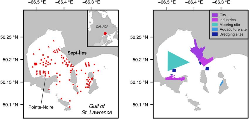
Dreujou et al.                                                                                    Ecosystem Status of an Anthropized Sub-Arctic Area

Secretariat of the CBD, 2010; SDG, 2015). The management of               as density and biomass of individuals—to infer community
ecosystems requires an understanding of how habitats and                  status. Relationships between abundance and a community
communities respond to drivers of change, i.e., forces that               status have frequently been discussed, as species do not have
affect environmental processes and modify ecosystem state from            the same tolerance to disturbance (Pearson and Rosenberg,
equilibrium (Boonstra et al., 2015; Beauchesne et al., 2020; Orr          1978). As such, the use of abundance-biomass curves has been
et al., 2020). In addition to natural drivers (e.g., temperature          proposed to detect if communities are in a balanced state, where
anomalies, freshwater inputs, hypoxic events), influences from            K-selected taxa are dominant, compared to a disturbed state, with
human activities (e.g., fisheries, chemical pollution, species            a dominance of r-selected taxa (Pearson and Rosenberg, 1978;
introductions) are also considered as ecosystem drivers. As               Gray, 1979; Warwick and Clarke, 1994). Category 2 indicators are
natural and anthropogenic drivers may affect ecosystems                   biodiversity parameters, i.e., community characteristics such as
concomitantly, it is important to understand how both relate to           taxa identity and prevalence, which allow complex information
observed effects (Brown et al., 2014). To tackle these questions,         to be aggregated into a unique metric. Finally, indicators in
environmental assessments rely on the best available knowledge,           Category 3 are computed based on variations of responses of
acquired through ecological groundwork in ecosystems of                   taxa to disturbance. Pioneer works by Pearson and Rosenberg
interest (such as biodiversity surveys, time series monitoring or         (1978) proposed a model of benthic community evolution along
experimental studies), and on the communication of results to             a gradient of organic enrichment, laying the path toward a set of
a wide range of stakeholders (Borja et al., 2012; Borja, 2014;            indicators that relate community structure and ecological status.
Chapman, 2016; Teixeira et al., 2016). Because such assessments              Environmental indicators, such as the AZTI Marine Biotic
are important foundations for decision makers, it is essential to         Index or the Infaunal Trophic index, have been applied
properly account for the inherent complexity and variability of           in a number of North American ecosystems, including
ecological data.                                                          Chesapeake Bay, Willapa Bay and the Southern California coast
    The use of integrative methods, such as indicators, is                (United States), but efficiency to detect perturbation has been
particularly relevant in this context. An indicator of ecological         mixed (Word, 1978; Maurer et al., 1999; Ferraro and Cole,
status is defined as a quantitative measure that synthesizes              2004; Borja et al., 2008b; Pelletier et al., 2018). Less commonly,
ecosystem information to infer ecosystem status (Rice,                    studies on the Pacific and Atlantic coasts of Canada have also
2003; Rees et al., 2008). Many holistic frameworks, such as               evaluated the utility of existing indicators, although these studies
ecosystem-based management, marine spatial planning and                   have most often found poor performance (Sutherland et al.,
DPSIR (Driver Pressure State Impact Responses) models,                    2007; Burd et al., 2008; Callier et al., 2008; Robert et al., 2013).
have included indicators in their methodology (Smeets and                 There is thus a need to test and validate indicators for Canadian
Weterings, 1999; Niemi and McDonald, 2004; European                       ecosystems, in particular by comparing outcomes and efficiency
Commission, 2008; Rees et al., 2008; Levin et al., 2009; Atkins           of existing methods, which will greatly benefit to tackle ecosystem
et al., 2011; Borja et al., 2013, 2015, 2016; Santos et al., 2019).       management objectives within Canada’s Ocean Act and the
However, environmental indicators evaluate specific ecosystem             Oceans Strategy (Government of Canada, 1996; Department of
components, perturbations and/or spatiotemporal scales,                   Fisheries and Oceans, 2002).
potentially limiting their applicability in other systems, thus              To this end, we evaluated various indicators of ecological
leading to the development of many indicators worldwide (Niemi            status in a coastal industrial harbor area, where human activities
and McDonald, 2004; Pinto et al., 2009; Teixeira et al., 2016).           may significantly impact local benthic ecosystems. Industrial
    One of the ecosystem components most frequently selected              harbor areas are regions regrouping significant industrial
for environmental indicators are macrobenthic invertebrates,              activities coupled with harbor platforms linking production with
as they play an important role in the structure and functioning           commercial shipping routes worldwide. We selected the region
of benthic marine ecosystems (Dauvin and Ruellet, 2007; Pratt             of Sept-Îles (Québec, Canada) for this study. Located in the
et al., 2014). Examples of this include engineering species               Gulf of St. Lawrence, one of the management areas designated
(e.g., structural features for other species, bioturbation) and           by Fisheries and Oceans Canada and a major strategic region
interactions with nutrient cycles (e.g., nutrient sequestration           for Québec (Department of Fisheries and Oceans, 2009; Daigle
in sediments, remineralization, benthic-pelagic coupling)                 et al., 2017; Schloss et al., 2017; Ferrario and Archambault,
(Largaespada et al., 2012; Link et al., 2013; Belley et al., 2016;        in preparation), Sept-Îles is the fourth largest Canadian port in
Bourque and Demopoulos, 2018). Many macrobenthic species                  2019 in terms of total exchanged goods and the second largest
are characterized by a sedentary lifestyle and a relatively long          in Québec (Statistics Canada, 2011; Binkley, 2020). Industrial
life span, which is particularly interesting when studying human          activities at Sept-Îles are largely focused on international shipping
influence as communities will reflect medium-term conditions,             of iron ore mined in northern Québec and Labrador, the
resulting in adaptation or local extinction (e.g., Dauer, 1993;           production of aluminum and various fisheries operate in the bay
Borja et al., 2000; Wei et al., 2020).                                    (Department of Fisheries and Oceans, 2019).
    As pointed out by Rice (2003) and Salas et al. (2006),                   The objectives of this study are to (i) compare outcomes
environmental indicators may be classed into categories                   of various environmental indicators on benthic ecosystems of
according to their methodological basis, including three main             the Sept-Îles region and (ii) understand how these indicators
categories used in environmental assessments. Category 1                  relate to habitat parameters for validation and to select
regroups indicators based on measures of abundance—such                   appropriate applications.

Frontiers in Marine Science | www.frontiersin.org                     2                                       March 2021 | Volume 8 | Article 637546
Dreujou et al. Ecosystem Status of an Anthropized Sub-Arctic Area
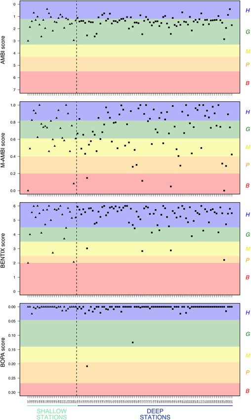
FIGURE 1 | Map of the study area. (A) Location of the sampled stations, with light blue triangles and dark blue squares representing shallow (< 15 m) and deep (>
15 m) stations, respectively, (B) Location and identity of human activities present in the area.
MATERIALS AND METHODS Sept Îles) and one type of community (individuals higher than
0.5 mm) were considered.
Study Area A total of 108 stations were selected in the study area, using
We targeted ecosystems with a sandy-silty sediment in the a randomization algorithm to cover the full extent of the sector,
industrial harbor area of Sept-Îles (Côte-Nord region of Québec, constrained between 0 and 80 m deep, and with increased
Canada), which considers ecosystems in the Baie des Sept Îles and sampling effort in areas with human activities (Figure 1A).
the archipelago at its entrance (Figure 1A; Dreujou et al., 2018, Himmelman (1991) showed that benthic communities in the
2020). Coasts are characterized by sandy beaches, tidal marshes Northern Gulf of St. Lawrence above and below 15–20 m
and anthropogenic structures. Mean depth is 35 m in the bay and deep differ. Likewise, preliminary fieldwork in the study region
can reach up to 150 m in the archipelago (Dutil et al., 2012). It is detected a thermocline in the water column at ca. 15 m deep.
influenced by freshwater inputs from multiple streams and strong Consequently, we discriminated two groups of stations in order
tidal currents resulting in a mixed water column and an estuarine to ensure habitat homogeneity within depth classes: shallow (15 m, 82 stations). We
considered sub-Arctic due to the formation of ice on the shore in sampled the benthic ecosystem in July 2017, using a Ponar grab
November/December and in the bay in January/February, along (0.05 m2 ) deployed from a boat, with two independent casts
with an important freshwater run-off due to snowmelt in April at each station.
(Demers et al., 2018). The first cast collected two subsamples—one for the analyses
This region hosts several human activities, including of organic matter content and another for sediment grain size—
industrial, commercial and dredging operations located at the stored at -20◦ C until processing in the laboratory. The percentage
City of Sept-Îles and the Pointe-Noire sector (on the southern of total organic matter (i.e., sum of organic carbon and organic
section of Baie des Sept Îles), along with an aquaculture site nitrogen) in the sediment was determined using the Loss-on-
and various fisheries throughout the bay (Figure 1B). Many Ignition method (Davies, 1974). Grain-size analysis was done on
projects have been done in this region to characterize pelagic a sieving column for the fraction with particles larger than 2 mm
and benthic communities and habitats in relation to coastal and with a Laser Diffraction Particle Size Analyzer for the smaller
stressors (Canadian Healthy Oceans Network, 2016; Carrière, fractions. Results from both techniques were combined to yield a
2018; Dreujou et al., 2020). unified size distribution range from 0.04 µm to 26.5 mm. From
this, percentages of gravel, sand, silt and clay were calculated as
defined by Wentworth (1922) and Folk (1980).
Benthic Ecosystems Sampling All sediment obtained from the second cast was sieved
The sampling design and methods used to collect and analyze on a 0.5 mm mesh size and preserved in a solution of
ecological samples were similar to those presented in Dreujou BORAX-buffered formalin (4%) solution for subsequent benthic
et al. (2020), with the exception that only one region (Baie des macrofauna identification (Dreujou et al., 2020). The resulting
Frontiers in Marine Science | www.frontiersin.org 3 March 2021 | Volume 8 | Article 637546Dreujou et al. Ecosystem Status of an Anthropized Sub-Arctic Area
samples were sorted using a stereomicroscope and taxa identified diversity), D6 (seafloor integrity), and D8 (contaminants) of
to the lowest taxonomic level possible with reference manuals Good Environmental Status (European Commission, 2008; Borja
and identification guides; names were validated according to et al., 2013), choosing those that applied to benthic invertebrates
the World Register of Marine Species (WoRMS Editorial Board, in soft-bottom habitats. We considered each station separately,
2020). Taxon density and biomass per grab were recorded by allowing an assessment of the spatial variability and mean
counting and weighting (blotted wet mass) individuals in each for each indicator, and when possible we pooled all stations
sample, respectively. together to obtain an estimate for the bay-scale system. We
In addition to these parameters, we considered estimates of used R v4.0 to perform data manipulations and calculations
heavy metal concentrations in the sediment. Concentrations at (R Core Team, 2020).
the sampled stations were calculated based on values obtained We included in Category 1 the total density (number of
in the same area in 2014 and 2016, retrieved from a database individuals collected per grab), total biomass (wet mass of
hosted by Carrière (2018), using Inverse Distance Weighting individuals collected per grab), and the W-Statistic Index,
interpolation (Dale and Fortin, 2014). We focused on metals for calculated based on abundance-biomass curves for the
which toxicity criteria have been defined in the Biological Effects community (Warwick and Clarke, 1994). Those indicators were
Database for Sediments (Environment Canada and Ministère computed using benthic taxa abundance sampled at each station.
du Développement Durable de l’environnement et des Parcs du For Category 2, we considered taxa richness (number of
Québec, 2007; Centre d’Expertise en Analyse Environnementale collected taxa) and related metrics to describe the community’s
du Québec, 2014): arsenic, cadmium, chromium, copper, structure and the relative prevalence of taxa within it, such
mercury, lead and zinc; we also included iron and manganese to as the Shannon index, Margalef index, Simpson index, and
account for possible contamination from local ore industries. Pielou evenness (Legendre and Legendre, 1998; Magurran and
McGill, 2011). We also considered taxonomic and functional
Environmental Indicator Calculation diversities, based on taxonomic relationships between taxa and
Indicators of ecological status were selected from Pinto et al. information about biological traits, respectively (Warwick and
(2009), DEVOTES (2012), and Teixeira et al. (2016), and grouped Clarke, 1995; Clarke and Warwick, 1998; Mason et al., 2005;
into three Categories according to their methodology (Table 1). Villéger et al., 2008). Taxa richness, Shannon index, Margalef
We targeted indicators related to descriptors D1 (biological index, Simpson index, and Pielou evenness were calculated using
the benthic community at each station. For taxonomic diversity,
we gathered relatedness data for taxa using the WoRMS online
database (WoRMS Editorial Board, 2020). To estimate functional
TABLE 1 | Summary of the evaluated indicators.
diversity, we computed functional richness, functional evenness
Indicator Unit Range References used and functional divergence (Mason et al., 2005; Villéger et al.,
2008) by considering five biological traits—body composition,
Category 1—Abundance measures
body size, feeding type, mobility and lifestyle—with a total of 26
Total density ind.grab−1 [0; +∞[ –
modalities (Table 2). Because taxa can present several modalities
Total biomass gWM.grab−1 [0; +∞[ –
for a trait, we assigned a continuous value between 0 (absence
W-Statistic index NA [–1; 1] Warwick and Clarke, 1994
of the modality) and 1 (presence of the modality) for each taxon
Category 2—Diversity measures
and each trait (the sum of values for every modality within a
Specific richness Taxa [0; +∞[ –
trait equals 1). Biological trait data was extracted from WoRMS,
Shannon index NA [0; 5] Magurran and McGill, 2011
SealifeBase, the Encyclopedia of Life, and Arctic Traits databases
Margalef index NA [0; +∞[ Magurran and McGill, 2011
as well as dedicated articles (Degen and Faulwetter, 2019; EoL,
Simpson index NA [0; 1] Magurran and McGill, 2011
2020; Palomares and Pauly, 2020; WoRMS Editorial Board, 2020).
Pielou evenness NA [0; 1] Magurran and McGill, 2011
R Packages vegan and FD were used to calculate indicators in
Taxonomic diversity NA [0; +∞[ Warwick and Clarke, 1995;
Clarke and Warwick, 1998 this category (Laliberté and Legendre, 2010; Laliberté et al., 2014;
Functional richness NA [0; +∞[ Mason et al., 2005; Villéger Oksanen et al., 2019).
et al., 2008 Finally, indicators in Category 3 included the AZTI Marine
Functional evenness NA [0; 1] Mason et al., 2005; Villéger Biotic Index (AMBI) and its multivariate version (M-AMBI),
et al., 2008 which are based on the relative proportion of taxa classified
Functional divergence NA [0; 1] Mason et al., 2005; Villéger into five ecological groups depending on their tolerance to
et al., 2008 perturbation (Grall and Glemarec, 1997; Borja et al., 2000;
Category 3—Characteristic species Muxika et al., 2007), BENTIX, where only two ecological
AZTI Marine Biotic NA [0; 7] Borja et al., 2000 groups are considered (Simboura and Zenetos, 2002), and the
Index (AMBI)
Benthic Opportunistic Polychaetes Amphipods Index (BOPA),
Multivariate Marine NA [0; 1] Muxika et al., 2007
Biotic Index (M-AMBI)
which compares proportions of opportunistic polychaetes and
BENTIX NA [0; 6] Simboura and Zenetos, 2002
amphipods (Dauvin and Ruellet, 2007). Sampled taxa were
Benthic Opportunistic NA [0; log(2)] Dauvin and Ruellet, 2007
assigned to ecological groups, from group I to V, based on
Polychaete Amphipod the list of Borja et al., version of May 2019 (AZTI, 2019;
index (BOPA) Supplementary Table S1). Because this list was developed for
Frontiers in Marine Science | www.frontiersin.org 4 March 2021 | Volume 8 | Article 637546Dreujou et al. Ecosystem Status of an Anthropized Sub-Arctic Area
TABLE 2 | Summary of the functional traits and modalities. We computed the Ecological Quality Ratios for Category 3
indicators. This ratio compares the value of an indicator to
Biological trait Modality
a reference, such as a targeted state or unperturbed/pristine
Body composition Non-calcified tissue ecosystem, so that an Ecological Quality Status can be assigned
Calcareous (not specified) (five categories: “bad,” “low,” “moderate,” “good,” and “high”
Calcareous—calcium carbonate status). The formula to compute the Ecological Quality Ratio is
Calcareous—amorphous calcium carbonate the following (Bund and Solimini, 2007):
Calcareous—aragonite
Calcareous—calcite
Vind −Rbad
EQR =
Calcareous—high magnesium calcite Rhigh −Rbad
Chitinous
Body length Small (10 mm)
Limits between each Ecological Quality Status class are specific
Feeding type Surface deposit feeder
to the indicator used (Borja et al., 2000; Simboura and Zenetos,
Subsurface deposit feeder
2002; Muxika et al., 2005, 2007; Dauvin and Ruellet, 2007).
Filter/suspension feeder
Finally, we explored covariation between indicators
Grazer
and habitat parameters (organic matter content, grain size
Predator
distribution and heavy metal concentrations), using scatterplots
Scavenger
for each pair of variables. Correlation was assessed with
Parasite
Spearman’s rank coefficients to understand the relevance
Mobility Sessile
of each indicator to the computation of ecological status
Limited (Quinn and Keough, 2002).
Mobile
Lifestyle Fixed
Tubicolous
RESULTS
Burrower
Crawler Overview of Benthic Habitats and
Swimmer Communities
Sediment was mostly composed of sand and silt fractions,
with concentrations of organic matter rarely surpassing 3%
(Supplementary Table S3). Heavy metal concentrations did not
European taxa, we assigned groups to unregistered taxa based on
reach high toxicity levels as defined by Environment Canada
species physiology studies and taxonomic relationships (Pelletier
(Environment Canada and Ministère du Développement Durable
et al., 2018). We used this list to further regroup taxa to a
de l’environnement et des Parcs du Québec, 2007; Centre
“sensitive” (groups I and II) and a “tolerant” (groups III to
d’Expertise en Analyse Environnementale du Québec, 2014;
V) metagroup to compute BENTIX (Simboura and Zenetos,
Dreujou et al., 2020; Supplementary Table S3). A total of 132 taxa
2002), and to obtain the proportion of opportunistic polychaetes
were identified, belonging to eight phyla, with a dominance of
(groups III to V) and sensitive amphipods (group I) to calculate
arthropods, mollusks, and annelids (Supplementary Table S1).
BOPA (Dauvin and Ruellet, 2007; Supplementary Table S1).
The most abundant taxa were the polychaete Micronephthys
M-AMBI was calculated using the dedicated software AMBI
neotena, the cumacean Eudorellopsis integra, the amphipod
v5.0 (AZTI, 2019), where “bad” and “high” status conditions are
Protomedeia grandimana, Nematoda (adults), and the bivalve
required for taxa richness, Shannon index and AMBI (Muxika
Macoma calcarea (Supplementary Table S1). From this list, no
et al., 2007). Because historical data on benthic invertebrates is
species which can be considered as exotic to this region have been
scarce in our study area, we used the outcomes of our sampling
reported (Simard et al., 2013).
to establish these values by selecting the 5 and 95 percentiles of
the variable distribution (for “bad” and “high” status, respectively,
Supplementary Table S2) (Buchet, 2010). Indicator Outcomes
Category 1 Indicators
Indicators in this category presented greater mean values in
Integration and Statistical Analysis deep than shallow stations, with the exception of total density
Results for each indicator were reviewed qualitatively and (Table 3). Shallow stations showed a higher total density than
compared to benthic ecosystem data in the Gulf of St. Lawrence, deep stations, but this may be an outlier effect due to a
when available. Robustness for indicators in Categories 1 and 2 single station close to the City of Sept-Îles (Supplementary
was calculated as the 95% confidence interval using a resampling Figures S1A–C), where density was 899 individuals.grab−1 with
routine (bootstrap, 1000 replicates), and the difference between a dominance of P. grandimana. Overall, shallow and deep stations
averages of each indicator and the resampling averages (i.e., presented low total biomass, except for a couple of stations
bootstrap bias). due to the presence of the echinoderms Echinarachnius parma
Frontiers in Marine Science | www.frontiersin.org 5 March 2021 | Volume 8 | Article 637546Dreujou et al. Ecosystem Status of an Anthropized Sub-Arctic Area
TABLE 3 | Values of the mean and standard error (SE) for each indicator, the difference between bootstrapped mean and the true mean (bias) and the 95% confidence
interval (CI), for shallow and deep stations.
Shallow stations (n = 26) Deep stations (n = 82)
Indicator Bay-scale Mean (SE) Bias 95% CI Bay-scale Mean (SE) Bias 95% CI
Category 1
Total density 3606 138.7 (36.3) 0.38 [136.9; 141.3] 7309 89.13 (7.6) 0.16 [88.81; 89.77]
Total biomass 191.16 7.35 (4.2) 0.057 [7.14; 7.68] 715.06 8.72 (2.3) 0.024 [8.55; 8.84]
W-Statistic index 0.13 0.011 (0.003) 0.016 [0.027; 0.028] 0.11 0.025 (0.002) 0.008 [0.033; 0.033]
Category 2
Specific richness 65 9.19 (0.9) 0.036 [9.17; 9.29] 117 13.99 (0.5) 0.009 [13.96; 14.03]
Shannon index 2.67 1.353 (0.1) 0.007 [1.354; 1.366] 3.18 1.952 (0.05) 0.0002 [1.949; 1.955]
Margalef index 7.81 1.92 (0.1) 0.014 [1.93; 1.95] 13.04 3.05 (0.1) 0.0001 [3.04; 3.05]
Simpson index 0.88 0.62 (0.04) 0.003 [0.62; 0.63] 0.92 0.77 (0.02) 0.0002 [0.77; 0.77]
Pielou evenness 0.64 0.65 (0.05) 0.004 [0.657; 0.663] 0.67 0.76 (0.02) 0.0003 [0.76; 0.76]
Taxonomic diversity 68.48 51.66 (3.8) 0.357 [51.79; 52.25] 74.8 63.48 (1.3) 0.014 [63.39; 63.55]
Functional richness – 23.35 (4.6) 3.171 [26.11; 26.93] – 31.76 (2.5) 7.59 [38.83; 39.88]
Functional evenness – 0.554 (0.04) 0.002 [0.55; 0.554] – 0.632 (0.01) 0.002 [0.633; 0.635]
Functional divergence – 0.77 (0.05) 0.007 [0.77; 0.78] – 0.83 (0.01) 0.011 [0.82; 0.82]
Category 3
AMBI 1.57 1.5 (0.1) – – 1.53 1.45 (0.05) – –
M-AMBI – 0.68 (0.05) – – – 0.7 (0.03) – –
BENTIX 5.15 4.95 (0.2) – – 5.25 5.31 (0.09) – –
BOPA 0.002 0.003 (0.001) – – 0.004 0.007 (0.003) – –
AMBI, AZTI Marine Biotic Index; M-AMBI, Multivariate AZTI Marine Biotic Index; BOPA, Benthic Opportunistic Polychaetes Amphipods Index.
and Strongylocentrotus sp. (Supplementary Figures S1A–C). The organisms for mobility and burrowers for lifestyle, at both
W-Statistic Index was positive and close to zero at nearly all shallow and deep stations.
shallow and deep stations (Supplementary Figures S1A–C) and
the abundance-biomass curve presented higher abundance than Category 3 Indicators
biomass values when species were ranked (Figure 2). Classification of taxa into ecological groups to compute Category
3 indicators yielded 51 taxa in group I (sensitive to disturbance,
38.6% of the taxa), 63 in group II (indifferent to disturbance,
Category 2 Indicators 47.7%), 11 in group III (tolerant to disturbance, 8.3%), 1 in
Category 2 indicators showed similar trends for shallow and each of groups IV and V (second- and first-order opportunists,
deep stations, while being generally higher for the latter respectively, 0.8%) and 5 were not assigned due to a too broad
(Table 3). In particular, there is a close similarity between the taxonomic resolution (Supplementary Table S1). This classified
spatial distributions of taxa richness, Shannon and Margalef 114 taxa in the “sensitive” group and 13 in the “tolerant”
indices and taxonomic diversity (Supplementary Figures S1D– group (Supplementary Table S1). Concerning polychaetes
L). Variability for shallow stations is quite low, except for a station and amphipods, we observed four opportunistic polychaetes
in front of Pointe-Noire where only one taxon was present, (Cossura longocirrata, Eteone sp., Hediste diversicolor, Praxillella
while deep stations tend to display the highest values in the praetermissa) and nine sensitive amphipods (Ameroculodes
archipelago compared to the center of the bay (Supplementary edwardsi, Ampelisca vadorum, Byblis gaimardii, Lysianassidae,
Figures S1D–L). Mean values for the Simpson index and Pielou Maera danae, Phoxocephalus holbolli, Pontoporeia femorata,
evenness reached 0.62 (standard error of 0.04) and 0.77 (0.02), Quasimelita formosa, Quasimelita quadrispinosa).
respectively, for shallow stations and 0.66 (0.05) and 0.76 (0.02) An AMBI score of 1.57 and 1.53 was obtained for the bay-
for deep stations (Table 3). The same relationship between scale estimate at shallow and deep stations, respectively, which
shallow and deep stations is observed for these metrics, even corresponds to a “slight imbalance” site classification (Borja
though the distribution for both is skewed with some stations et al., 2000). Overall, low AMBI values were obtained at each
closer to coasts presenting very low values (Supplementary station, being 1.5 on average (standard error of 0.13) for shallow
Figures S1D–L). Concerning functional diversity, deep stations stations and 1.45 (0.05) for deep stations, and never exceeding
presented higher mean functional richness, functional evenness 3, and no particular spatial trend can be observed (Table 3
and functional divergence relative to those at shallow stations and Supplementary Figures S1M–P). The bay-scale M-AMBI
(Table 3). The most abundant modality for each biological trait could not be computed with the percentile method, and at the
was non-calcified tissue for body composition, small individuals station level, generally high mean values of 0.68 (0.05) and 0.7
for body size, surface deposit-feeders for feeding type, mobile (0.03) were observed for shallow and deep stations, respectively
Frontiers in Marine Science | www.frontiersin.org 6 March 2021 | Volume 8 | Article 637546Dreujou et al. Ecosystem Status of an Anthropized Sub-Arctic Area
FIGURE 2 | Values of abundance and biomass for ranked species (logarithm scale), for shallow stations and deep stations.
(Table 3). Stations outside of the bay tended to be characterized richness where it reached 3.17 and 7.59, respectively (Table 3),
by higher values than those inside it, especially close to the demonstrating a relatively high robustness of the indicators.
coast and in the northern section of the bay, but this may The true mean was included in the 95% confidence interval for
be related to the spatial distribution of taxa richness and the five indicators at shallow stations (taxa richness, total density,
Shannon index (Supplementary Figures S1M–P). The BENTIX total biomass, functional evenness, functional divergence) and
bay-scale estimate was 5.15 for shallow stations and 5.25 for deep eight at deep stations (taxa richness, total density, total biomass,
stations, while at the station-level mean values were 4.95 (0.23) Shannon index, Margalef index, Simpson index, Pielou evenness,
and 5.31 (0.09), respectively (Table 3). These values correspond to taxonomic diversity) (Table 3).
a “normal/pristine” pollution classification for the majority of the The analysis of covariation between indicators reported
area sampled, except for some stations close to coasts (Simboura moderate to very high Spearman’s coefficients (0.22 < |ρ| < 0.96)
and Zenetos, 2002). Finally, BOPA produced low scores of 0.002 (Table 4). Category 2 indicators presented the highest proportion
and 0.004 for shallow and deep bay-scale estimates, respectively, of within-Category significant correlations at both shallow
similar to means of 0.0028 (0.0012) for shallow and 0.0067 (0.003) and deep stations (Table 4). The vast majority of these
for deep stations, respectively (Table 3), denoting “high status” correlations were positive, with the strongest correlations
classifications. Only two stations had a score higher than 0.05, between Shannon and Margalef indices, and were represented
a trend that is not shared with neighboring stations, which may by linear proportionality between indicators on the scatterplots.
indicate localized low-intensity perturbations (Supplementary Category 2 indicators were also frequently correlated to
Figures S1M–P). indicators from Categories 1 and 3, especially for the W-Statistic
Calculation of Ecological Quality Ratios using Category 3 Index and the M-AMBI (Table 4). The latter Categories did
indicators produced similar results for AMBI, BENTIX and not present high within-Category correlations, except between
BOPA (Figure 3). The majority of stations (shallow and deep) AMBI/BENTIX and M-AMBI/BOPA at shallow stations, and the
presented a “high” or “good” ecological status except for a few W-Statistic Index and AMBI at deep stations.
stations with a “poor” status (Figure 3). In contrast, results for
M-AMBI were less uniform, with a high variation among both Relationships With Habitat Parameters
shallow and deep stations, such that no general trends may be Correlations between Category 1 indicators and abiotic
highlighted (Figure 3). parameters detected non-significant relationships with sediment
parameters (except between the W-Statistic Index and gravel
Robustness and Covariation and sand contents at deep stations), while they were significant
For Category 1 and 2 indicators, bootstrap bias was low at both and negative between most heavy metals and total density
shallow and deep stations (less than 0.4), except for functional and total biomass at shallow stations, and the W-Statistic
Frontiers in Marine Science | www.frontiersin.org 7 March 2021 | Volume 8 | Article 637546Dreujou et al. Ecosystem Status of an Anthropized Sub-Arctic Area FIGURE 3 | Values of Category 3 indicators ranked according to Ecological Quality Ratios, calculated for shallow and deep stations. (A) Calculated with the AZTI Marine Biotic Index (AMBI), (B) Calculated with the Multivariate AZTI Marine Biotic Index (M-AMBI), (C) Calculated with the BENTIX, (D) Calculated with the Benthic Opportunistic Polychaetes Amphipods Index (BOPA). B = “bad” status (red), P = “poor” status (orange), M = “moderate” status (yellow), G = “good” status (green), H = “high” status (blue). Index at deep stations (Table 5). The absolute value of highlighting relatively strong relationships, while they were Spearman’s rank coefficients was high for total density and less for the W-Statistic Index at deep stations (between total biomass at shallow stations (between −0.4 and −0.61), −0.22 and −0.29). Frontiers in Marine Science | www.frontiersin.org 8 March 2021 | Volume 8 | Article 637546
Dreujou et al.                                                                                                      Ecosystem Status of an Anthropized Sub-Arctic Area

TABLE 4 | Spearman rank correlation coefficients between indicators, for shallow and deep stations.

                        Category 1                                             Category 2                                                     Category 3

Indicator        TD        TB        W        S       H        M        λ          J         1      FR        FE       FD       AMBI     M-AMBI       BENTIX      BOPA

Shallow stations
Category 1
TD
TB                –
W                 –         –
Category 2
S                0.77      0.43       –
H                 –         –        0.62    0.58
M                 –         –        0.53    0.76    0.81
λ                 –         –        0.68     –      0.89     0.61
J            −0.66          –        0.59     –      0.46      –        0.7
1            −0.44          –        0.71     –      0.59     0.48      0.75      0.86
FR               0.8       0.5        –      0.87     –       0.58       –       −0.41       –
FE                –         –        0.67     –      0.58     0.41      0.65      0.54      0.51      –
FD                –         –         –      0.41     –        –         –         –         –        –        –
Category 3
AMBI              –       −0.42       –       –       –        –         –         –         –        –        –         –
M-AMBI            –        0.48       –      0.8     0.78     0.86      0.5        –         –      0.64      0.4      0.43       –
BENTIX            –         –         –       –       –        –         –         –         –        –        –         –     −0.78          –
BOPA              –         –         –      0.45     –       0.41       –         –         –        –        –         –        –         0.53          –
Deep stations
Category 1
TD
TB                –
W            −0.31         0.35
Category 2
S                0.58       –        0.37
H                 –         –        0.75    0.67
M                 –         –        0.61    0.9     0.86
λ            −0.23          –        0.75    0.47    0.96     0.7
J            −0.67          –        0.63     –      0.64     0.29      0.79
1            −0.39          –        0.69    0.28    0.81     0.57      0.89      0.88
FR               0.35       –        0.32    0.71    0.46     0.67      0.33       –         –
FE           −0.55          –        0.42     –       –        –        0.31      0.59      0.43      –
FD                –         –     −0.32     −0.27   −0.39   −0.37     −0.41      −0.39     −0.5    −0.28       –
Category 3
AMBI              –         –     −0.29       –     −0.25   −0.23     −0.28      −0.31     −0.3       –        –       0.32
M-AMBI            –         –        0.64    0.79    0.87     0.89      0.76      0.39      0.6     0.58       –      −0.4     −0.52
BENTIX            –         –         –       –       –        –         –         –         –        –        –      −0.24    −0.7           –
BOPA              –         –         –       –       –        –         –         –       −0.22      –        –         –        –           –           –

Only significant relationships of the triangular matrix are presented. TD, total density, TB, total biomass; W, W-Statistic index; S, taxa richness; H, Shannon index; M,
Margalef index; λ, Simpson index; J, Pielou evenness; 1, taxonomic diversity; FR, functional richness; FE, functional evenness; FD, functional divergence; AMBI, AZTI
Marine Biotic Index; M-AMBI, Multivariate AZTI Marine Biotic Index; BOPA, Benthic Opportunistic Polychaetes Amphipods Index.

   For Category 2 indicators, correlations with sediment                                 correlations. The vast majority of these relationships were
parameters were significant only for some cases involving taxa                           moderate to high (between −0.22 and −0.45), except at deep
richness, the Margalef index, taxonomic diversity and functional                         stations for gravel and sand contents and between functional
richness (Table 5). Relationships with heavy metals were detected                        divergence and some heavy metals.
mainly at deep stations, in particular for cadmium, copper,                                 Finally, several significant relationships were observed
lead and zinc; at shallow stations, functional richness showed                           between Category 3 indicators and sediment parameters (organic
significant correlations with all heavy metals except cadmium,                           matter, sand and silt contents), including at shallow stations for
while functional divergence and taxa richness presented marginal                         AMBI and BENTIX and at deep stations for BENTIX and BOPA

Frontiers in Marine Science | www.frontiersin.org                                   9                                            March 2021 | Volume 8 | Article 637546
Dreujou et al. Ecosystem Status of an Anthropized Sub-Arctic Area
TABLE 5 | Spearman rank correlation coefficients between environmental indicators and habitat parameters, for shallow and deep stations.
Sediment parameters Heavy metal concentrations
Indicator OM Gravel Sand Silt Clay As Cd Cr Cu Fe Mn Hg Pb Zn
Shallow stations
Category 1
TD – – – – – −0.46 – −0.52 −0.55 −0.49 – −0.52 −0.55 −0.52
TB – – – – – −0.42 −0.42 −0.59 −0.51 −0.39 −0.53 – −0.5 −0.61
W – – – – – – −0.4 – – – – – – –
Category 2
S – – – – – −0.47 – – – – – −0.39 – –
H – – – – – – – – – – – – – –
M – – – – – – – – – – – – – –
λ – – – – – – – – – – – – – –
J – – – – – – – – – – – 0.42 – –
1 – – – – – – – – – – – – – –
FR – – – – – −0.43 – −0.5 −0.43 −0.47 −0.46 −0.5 −0.42 −0.47
FE – – – – – – – – – – – – – –
FD – – – – – −0.6 – – – – – – −0.4 −0.4
Category 3
AMBI −0.43 – 0.47 −0.47 – – – – – – – – – –
M-AMBI – – – – – – – – – – – – – –
BENTIX 0.45 – – – – – – – – – – – – –
BOPA – – – – – – – – – – – – – –
Deep stations
Category 1
TD – – – – – – – – – −0.23 – – – –
TB – – – – – – – – – – – – – –
W – 0.24 −0.22 – – −0.29 −0.29 −0.27 −0.24 −0.27 −0.26 – −0.28 −0.29
Category 2
S −0.25 – – – – −0.27 −0.32 −0.31 −0.32 −0.45 −0.31 – −0.3 −0.34
H – – – – – −0.29 −0.29 −0.33 −0.29 −0.36 −0.31 −0.25 −0.31 −0.31
M −0.26 – – – – −0.32 −0.33 −0.36 −0.37 −0.45 −0.36 −0.28 −0.35 −0.38
λ – – – – – −0.22 −0.23 −0.27 −0.22 −0.28 −0.25 −0.22 −0.26 −0.24
J – – – – – – – – – – – – – –
1 – – 0.23 −0.29 – −0.29 −0.32 −0.35 −0.35 −0.35 −0.34 −0.33 −0.34 −0.35
FR – 0.25 – – – −0.25 −0.32 −0.29 −0.32 −0.36 −0.29 −0.28 −0.27 −0.33
FE – – – – – – – −0.22 −0.25 – −0.27 −0.27 −0.24 −0.22
FD – – – – – – 0.28 – 0.29 – – 0.29 0.28 0.34
Category 3
AMBI – – – – – – – – – – – – – –
M-AMBI – – – – – −0.24 −0.3 −0.3 −0.27 −0.38 −0.28 – −0.28 −0.31
BENTIX 0.27 – −0.26 0.23 – 0.23 0.23 0.24 0.25 – – 0.23 – –
BOPA – – −0.31 0.34 – 0.33 0.28 0.36 0.31 0.33 0.38 0.3 0.33 0.3
Only significant relationships are presented. TD, total density; TB, total biomass; W, W-Statistic index; S, taxa richness; H, Shannon index; M, Margalef index; λ, Simpson
index; J, Pielou evenness; 1, taxonomic diversity; FR, functional richness; FE, functional evenness; FD, functional divergence; AMBI, AZTI Marine Biotic Index; M-AMBI,
Multivariate AZTI Marine Biotic Index; BOPA, Benthic Opportunistic Polychaetes Amphipods Index; OM, organic matter; As, arsenic; Cd, cadmium; Cr, chromium; Cu,
copper; Fe, iron; Mn, manganese; Hg, mercury; Pb, lead; Zn, zinc.
(Table 5). Organic matter was negatively correlated with AMBI −0.38), whereas correlations with BENTIX and BOPA were
values (coefficient of −0.43) at shallow stations and positively positive (between 0.23 and 0.36).
with BENTIX values at shallow and deep stations (0.45 and 0.27,
respectively); sand and silt contents had the opposite effect at
shallow stations for AMBI (0.47 and −0.47, respectively) and DISCUSSION
at deep stations for BENTIX (−0.26 and 0.23, respectively) and
BOPA (−0.31 and 0.34, respectively) values. Many relationships Strengths, Limitations, and Ecological
with heavy metals were detected at deep stations for all indicators Considerations of Indicators
except AMBI (Table 5). In particular, M-AMBI presented The analysis of benthic communities using Category 1 indicators
negative correlations with heavy metals (between −0.24 and relies on abundance relationships (either density or biomass
Frontiers in Marine Science | www.frontiersin.org 10 March 2021 | Volume 8 | Article 637546Dreujou et al. Ecosystem Status of an Anthropized Sub-Arctic Area
of individuals) without consideration of taxonomic identity. analysis, so that community-level effects are accurately described
Their calculation requires the least laboratory and analytical (Legendre and Legendre, 1998; Quinn and Keough, 2002;
time relative to the other calculated indicators. Deep stations Magurran and McGill, 2011).
present a higher density of benthic organisms than shallow Concerning functional diversity, functional richness is
stations, as predicted by patterns of coastal marine biodiversity generally lower at shallow stations and the two other indicators
(Gray and Elliott, 2009; Levinton, 2013; Piacenza et al., are in the same range, albeit being slightly greater at deep
2015). The abundance-biomass curve for shallow and deep stations. These results suggest that taxa at shallow stations have
stations is characteristic of an unstressed profile (Pearson and more specialized niches, i.e., less diverse functional strategies
Rosenberg, 1978; Warwick and Clarke, 1994), which is further (Villéger et al., 2008), indicating some redundancy of biological
supported by the W-Statistic Index being positive and close to traits. This property is linked to an increased ecosystem stability
0 at nearly all stations (Clarke, 1990). Studying communities and resilience, where possible extinctions due to perturbation will
through abundance relationships thus provides interesting results not modify the ecosystem structure even if some taxa disappear
concerning the status of the ecosystem, but the main assumption (Rosenfeld, 2002; Mouillot et al., 2013). However, bootstrap bias
behind indicators in this Category is that all species are equivalent was very high for this indicator, making conclusions less robust.
and have an identical role in the ecosystem structure and Moderate to high functional evenness and divergence denote
functioning. This, however is not necessarily true, as some that values for given biological traits are not evenly distributed
species can be considered “key species” in ecosystems due to and are skewed toward extremes (0 or 1). The consideration
unique engineering or trophic roles (e.g., Bond, 1994; Lawton of biological traits in addition to species identity allows to
and Jones, 1995). Thus, Category 1 indicators should be coupled study functions of the ecosystem, such as productivity, chemical
with ancillary methods focusing on biological characteristics elements cycling or energy transfers (Somerfield, 2008; Bellwood
of the species, such as life-history traits and physiological et al., 2019). This is an important addition to environmental
characteristics. assessments, as biological traits and adaptative responses to
Category 2 indicators focus on community biodiversity, disturbance are highly related (Mouillot et al., 2013; Miatta
granting additional detail than that provided by Category 1 et al., 2021). Indicators of functional diversity thus offer valuable
indicators. The notion of biodiversity can be interpreted along information to characterize communities in complement to
multiple points of view in an ecosystem, such as the diversity other Category 2 indicators, at the expense of increased analytical
of species, genes, habitats or functions (United Nations, 1992; time to assemble a traits database, for which information may be
Wilson, 1992; Hooper et al., 2005; Stachowicz et al., 2007). lacking or difficult to obtain.
While each targeted component has specific implications for For Category 3 indicators, community ecological status is
the ecosystem, high richness and high diversity values have assessed by considering the tolerance of taxa to perturbation.
generally been interpreted as signs of good ecological status Values for these indicators highlight an overall high status
(Covich et al., 2004; Borja et al., 2013). This statement needs in the study area, where taxa sensitive to perturbation are
to be considered carefully, as it is necessary to discuss results present without a dominance of opportunists, as illustrated
with comparable ecosystems and historical data so that diversity by the number of stations with a “high” Ecological Quality
trends are interpreted according to local background patterns Status. M-AMBI detected greater variability between stations
(Covich et al., 2004). relative to the other indicators, particularly within the bay.
Taxa richness indicated a quite diverse community, being A possible interpretation for this result may be the influence
nearly twice as great at deep stations, as expected given general of the percentile method used to compute “bad” and “high”
trends (Gray and Elliott, 2009; Levinton, 2013; Piacenza et al., status conditions for this indicator, advocating for a careful
2015). These numbers (132 taxa observed) are comparable to description of comparison conditions and a fortiori references
results from available benthic invertebrate surveys done in the values (Borja et al., 2012). Furthermore, classification into
study area, such as 27 taxa reported by OBIS (2020) in the Sept- ecological groups may introduce bias, as the list of Borja et al.
Îles region and 148 taxa by Nozères et al. (2015) in the Gulf of (2000) were primarily designed for European coastal ecosystems.
St. Lawrence. Results from diversity indicators (Shannon index, Inclusion of taxa found on Canadian coasts has been made
Margalef index, Simpson index, Pielou evenness and taxonomic based on taxonomic similarity with species already included in
diversity) showed moderate to high benthic diversity, with no the list, by reviewing studies on perturbation tolerance and by
dominance by any taxa (even distribution) and great taxonomic expert opinion, but these choices need to be ground-truthed
breadth. Few stations differ from this general trend, and those by dedicated ecological works. A wide spectrum of indicators
that do are mostly close to coasts where diversity is low and may be included within Category 3, as compiled by Pinto et al.
there is no clear evidence of perturbation. Diversity indicators are (2009) and Teixeira et al. (2016), and their use in environmental
frequently used in ecological studies to characterize communities assessments is linked to scientific and management objectives.
and to detect disturbance, which allows discussing their results Such indicators have been used with success in a variety of
building on a vast corpus of studies worldwide (Magurran and ecosystems (e.g., Borja et al., 2008a; Gillett et al., 2015), but
McGill, 2011). These univariate estimates, however, may mask they require a high volume of data to accurately relate taxa
individual responses arising for example from adaptation or and perturbation status, such as field observations, modeling of
changes in biotic relationships, and they should be coupled species distributions (native and non-indigenous), physiological
with multivariate methods, such as ordination or similarity studies and experimental work.
Frontiers in Marine Science | www.frontiersin.org 11 March 2021 | Volume 8 | Article 637546Dreujou et al. Ecosystem Status of an Anthropized Sub-Arctic Area
With these results, we can compare strengths and limitations from tidal currents), and (iii) perturbation effects may be more
of the calculated indicators. Category 1 indicators gather relevant pronounced on other components (such as phytoplankton or
baseline information on the ecosystem and requires the least time pelagic species).
to be computed. The downside is that it is difficult to discriminate Ecological indicators represent a valuable method to set
between anthropogenic perturbation and natural variability as conservation targets and to guide sustainable environmental
other community characteristics may be impacted and, most projects. In light of initiatives such as the Marine Strategy
importantly, they cannot be compared to reference conditions of Framework Directive, where indicators and descriptors have
ecological status. Category 2 indicators, such as the commonly been identified to monitor the ecological status of European
used Shannon index or Pielou evenness, are easy to compute from marine waters (European Commission, 2008; Borja et al., 2013,
well-built taxa lists, although taxonomic and functional diversity 2015, 2016), local stakeholders have the possibility to build on
demand more time to gather complementary information about these works to establish ecosystem-based management adapted to
phylogenetic relationships and ecosystem functions. However, Canadian ecosystems. Further research in other industrial coastal
the latter indicators provide more information on the community areas, including long-term monitoring, is needed to obtained
structure and are backed by ecological literature to infer a coherent and robust environmental assessments.
certain ecological status (Magurran and McGill, 2011). Finally,
Category 3 indicators demand the most time to be calculated, Validation and Limitations
in particular with the classification of taxa relative to their Assessing relationships between indicators highlighted
response to disturbance, but they have been specifically designed correlations, especially among Category 2 indicators. While
to determine Ecological Quality Ratios and to consider reference this does not necessarily imply causality in the interpretations,
conditions. Bias or uncertainty may be introduced during the covariation indicates that information gathered by some
classification process as extensive experimental groundwork is indicators is similar. This was expected for indicators relying
needed to properly assign taxa to groups, which is not always on specific ecosystem components to be computed, such as
available. Many of these indicators are region-specific, with M-AMBI and the Shannon index, both of which being a function
possible poor performance in other ecosystems (e.g., Callier et al., of taxa richness. With an environmental assessment perspective,
2008; Robert et al., 2013), so that further research is needed to these results show that calculation of some indicators will not
properly assess ecological status in sub-Arctic regions. provide additional information when the objective is to detect
trends in a targeted area. Understanding these links will allow
refining methodological protocols and to produce more efficient
Implications for Sept-Îles and Canadian and accurate assessments.
Ecosystems The use of ecological status indicators requires a validation
Sept-Îles is an important industrial harbor area for Québec, with procedure to ensure that outcomes are relevant (Dauvin et al.,
a variety of economic activities taking place in the bay and 2010; Heink et al., 2016; Burgass et al., 2017; Moriarty et al., 2018).
archipelago. All calculated indicators except M-AMBI pointed Because the region of Sept-Îles is not frequently represented
toward diverse benthic communities of generally good ecological in the scientific literature, it is then difficult to have baseline
status and no particular perturbation patterns have been detected data to validate ecosystem assessments. The studies of Dreujou
in the study area, which is coherent with previous descriptions et al. (2018, 2020) represent the only campaigns describing
of benthic ecosystems in this region (Carrière, 2018; Dreujou benthic habitats and communities in the Baie des Sept Îles, and
et al., 2020). When applying Category 3 indicators on the increased sampling would greatly improve indicator validation,
data from these studies, we obtained similar conclusions with in particular for Category 1 and 2 indicators where references
ecological status indicated as “good” to “high” for AMBI, conditions are currently not available. Inference of ecological
BENTIX and BOPA. status based on Category 3 indicators is relying on explicit
No particular trend has been observed for stations identified reference conditions for “bad” and “high” status. Defining values
as potentially impacted by Dreujou et al. (2020) in coastal regions for these conditions based on contemporary ecosystems will most
close to the City of Sept-Îles and Pointe-Noire, further suggesting certainly introduce bias, as most are likely to show some level of
an overall limited effect of perturbations. Compared to the degradation (which cannot be assessed), and alternatives, such as
regions where many of the assayed indicators were developed, historical datasets, are rare (Muxika et al., 2007; Borja et al., 2012).
e.g., in Atlantic and Mediterranean European ecosystems, the Overall, Category 1 and 2 indicators were relatively robust,
magnitude of human activity is considerably lower at Sept- with little difference between mean values calculated from the
Îles. As such, it is possible the range of variation induced by real and bootstrapped datasets (except for functional richness),
anthropogenic perturbation is not sufficient to severely impact indicating quite homogeneous results. The vast majority of
benthic ecosystems. This is even more relevant when we compare significant correlations between indicators and environmental
these results to other industrial harbor areas worldwide, where factors were found for heavy metal concentrations and most
human influence is more pronounced (e.g., Hewitt et al., 2005; such correlations were negative. This implies that indicators
Borja et al., 2006; Chan et al., 2016; Birch et al., 2020). Other would successfully detect perturbation due to heavy metal
hypotheses may explain this, such as (i) high community content, thus resulting in reduced ecological status, but fail
resilience and resistance, (ii) limitation of effective impacts to detect perturbations affecting other habitat parameters.
of activities by the dynamic of the ecosystem (e.g., flushing AMBI and BENTIX were correlated to organic matter content,
Frontiers in Marine Science | www.frontiersin.org 12 March 2021 | Volume 8 | Article 637546You can also read