Simulated reflectance above snow constrained by airborne measurements of solar radiation: implications for the snow grain morphology in the Arctic
←
→
Page content transcription
If your browser does not render page correctly, please read the page content below
Atmos. Meas. Tech., 14, 369–389, 2021
https://doi.org/10.5194/amt-14-369-2021
© Author(s) 2021. This work is distributed under
the Creative Commons Attribution 4.0 License.

Simulated reflectance above snow constrained by airborne
measurements of solar radiation: implications for
the snow grain morphology in the Arctic
Soheila Jafariserajehlou1,a,b , Vladimir V. Rozanov1 , Marco Vountas1 , Charles K. Gatebe2,3 , and John P. Burrows1
1 Instituteof Environmental Physics, University of Bremen, Bremen, Germany
2 Universities Space Research Association (USRA), Columbia, MD, USA
3 NASA Goddard Space Flight Center, Greenbelt, MD, USA
a now at: European Organisation for the Exploitation of Meteorological Satellites (EUMETSAT), Darmstadt, Germany
b now at: Rhea System GmbH, Darmstadt, Germany

Correspondence: Soheila Jafariserajehlou (jafari@iup.physik.uni-bremen.de)

Received: 25 February 2020 – Discussion started: 9 April 2020
Revised: 5 October 2020 – Accepted: 27 October 2020 – Published: 18 January 2021

Abstract. Accurate knowledge of the reflectance from             sults of this comparison are used to assess the quality and
snow/ice-covered surfaces is of fundamental importance           accuracy of the radiative transfer model in the simulation of
for the retrieval of snow parameters and atmospheric con-        the reflectance in a coupled snow–atmosphere system.
stituents from space-based and airborne observations.               Assuming that the snow layer consists of ice crystals with
   In this paper, we simulate the reflectance in a snow–         aggregates of eight column ice habit and having an effective
atmosphere system, using the phenomenological radiative          radius of ∼ 99 µm, we find that, for a surface covered by old
transfer model SCIATRAN, and compare the results with            snow, the Pearson correlation coefficient, R, between mea-
that of airborne measurements. To minimize the differences       surements and simulations is 0.98 (R 2 ∼ 0.96). For freshly
between measurements and simulation, we determine and            fallen snow, assuming that the snow layer consists of the
employ the key atmospheric and surface parameters, such as       aggregate of five plates ice habit with an effective radius
snow grain morphologies (or habits).                             of ∼ 83 µm and having surface inhomogeneity, the correla-
   First, we report on a sensitivity study. This addresses the   tion is ∼ 0.97 (R 2 ∼ 0.94) in the infrared and 0.88 (R 2 ∼
requirement for adequate a priori knowledge about snow           0.77) in the visible wavelengths. The largest differences be-
models and ancillary information about the atmosphere. For       tween simulated and measured values are observed in the
this aim, we use the well-validated phenomenological radia-      glint area (i.e., in the angular regions of specular and near-
tive transfer model, SCIATRAN. Second, we present and ap-        specular reflection), with relative azimuth angles < ±40◦ in
ply a two-stage snow grain morphology (i.e., size and shape      the forward-scattering direction. The absolute difference be-
of ice crystals in the snow) retrieval algorithm. We then de-    tween the modeled results and measurements in off-glint re-
scribe the use of this new retrieval for estimating the most     gions, with a viewing zenith angle of less than 50◦ , is gener-
representative snow model, using different types of snow         ally small ∼ ±0.025 and does not exceed ±0.05. These re-
morphologies, for the airborne observation conditions per-       sults will help to improve the calculation of snow surface re-
formed by NASA’s Cloud Absorption Radiometer (CAR).              flectance and relevant assumptions in the snow–atmosphere
   Third, we present a comprehensive comparison of the sim-      system algorithms (e.g., aerosol optical thickness retrieval al-
ulated reflectance (using retrieved snow grain size and shape    gorithms in the polar regions).
and independent atmospheric data) with that from airborne
CAR measurements in the visible (0.670 µm) and near in-
frared (NIR; 0.870 and 1.6 µm) wavelength range. The re-

Published by Copernicus Publications on behalf of the European Geosciences Union.
370                                    S. Jafariserajehlou et al.: Implications for the snow grain morphology in the Arctic

1   Introduction                                                  gion because its reflectance has an anisotropic nature, and
                                                                  the anisotropy increases with wavelength; (ii) unlike other
The extent and type of snow and ice cover have a signifi-         surface types (e.g., vegetation or soil) with a strong peak
cant impact on climate, as noted by Arrhenius over 100 years      in back-scattering direction (the hot spot effect), snow has
ago (Arrhenius, 1896). There is a positive feedback between       a strong forward peak for large viewing zenith angles (e.g.,
decreasing surface temperature, an increase in snow and ice       Gatebe and King, 2016); (iii) the snow reflectance varia-
cover, and an associated increase in planetary albedo, which      tion is larger in the principal plane (i.e., the plane contain-
then further decreases surface temperature and vice versa.        ing the Sun, surface normal, and observation direction) than
Consequently, changes in snow and ice extent and morphol-         in the cross plane (i.e., the one perpendicular to principal
ogy play a key role in climate change. Having accurate            plane; Warren, 1982; Lyapustin et al., 2010; Kokhanovsky
knowledge about snow/ice-covered surfaces is a prerequi-          and Breon, 2012). However, the remaining discrepancies
site for identifying and quantifying changes in the climate       between simulated reflectance in a snow–atmosphere sys-
(Schneider and Dickinson, 1974; Curry et al., 1995; Cohen         tem and field measurements led to further investigations in
et al., 2014; Kim et al., 2017; Wendisch et al., 2017, 2019).     the field of the single scattering properties of snow grains
   In addition, during recent decades, the Arctic region has      (Mishchenko et al., 1999; Jin et al., 2008; Yang and Liou,
warmed more rapidly than other regions. This phenomenon           1998; Yang et al., 2003, 2013), surface roughness (Warren
is known as the Arctic amplification (AA; Serreze and Barry,      et al., 1998; Hudson et al., 2006; Hudson and Warren, 2007;
2011). The analysis of the growing number of long-term            Lyapustin et al., 2010; Zhuravleva and Kokhanovsky, 2011),
records of the data products (e.g., the amount of trace gases,    and atmospheric-correction methods (Lyapustin et al., 2010).
aerosol, and cloud parameters) retrieved from passive and ac-     Despite substantial improvements, the uncertainties in our
tive satellite observations provides potentially invaluable in-   understanding of the microphysical and macroscopic prop-
formation for identifying and quantifying the evolution and       erties of snow are an unresolved issue for RTMs, ray tracing,
consequences of AA (Wendisch et al., 2017).                       and climate models. For example, the current state-of-the-art
   Because of the magnitude of the scattering from snow, the      RTMs yield much more anisotropic reflectance behavior for
use of remote sensing measurements above snow-covered             snow in the glint region than observed in reality (Zhuravl-
surfaces in the cryosphere requires accurate models of the        eva and Kokhanovsky, 2011; Lyapustin et al., 2010; Hud-
scattering and reflectance from snow surfaces. However,           son and Warren, 2007; Warren et al., 1998). These studies
the current differences between simulated and measured re-        either focus on the snow reflectance at the surface, employ-
flectance in a coupled snow–atmosphere system lead to sys-        ing an atmospheric-correction method (Leroux et al., 1998;
tematic errors in the determination of the atmospheric con-       Kokhanovsky and Zege, 2004; Kokhanovsky et al., 2005;
stituents, in particular for clouds and aerosol parameters but    Lyapustin et al., 2010; Negi and Kokhanovsky, 2011), or
also trace gases (e.g., Istomina et al., 2010; Istomina, 2012;    consider the atmospheric effects without in-depth investiga-
Jafariserajehlou et al., 2019).                                   tions of the surface parameters (Aoki et al., 1999; Hudson
   A large number of experimental and theoretical studies         et al., 2006; Kokhanovsky and Breon, 2012). A comprehen-
have been conducted measuring and modeling snow opti-             sive study and investigation of both the snow layer and atmo-
cal properties, such as the angular distribution of reflected     sphere parameters in a coupled snow–atmosphere system has
light over and within the snow surface and the subsequent         not yet been undertaken but is required to improve the accu-
derivation of snow albedo. The early measurements by Mid-         racy of remote sensing retrieval algorithms for aerosol and
dleton and Mungal (1952) and the model of Dunkle and Be-          cloud in the Arctic region (Istomina et al., 2010; Istomina,
vans (1956) used to analyze the transmittance and reflectance     2012; Jafariserajehlou et al., 2019).
of snow cover were the beginning of considerable efforts             The intent of this paper is to (i) study the sensitivity of
on this topic. Barkstrom (1972) formulated and solved the         scattering and reflectance in the coupled snow–atmosphere
scattering problem for snow surfaces in terms of the ra-          system to both surface and atmospheric parameters, (ii) re-
diative transfer theory. Later, the comparison of reflectance     trieve the most representative ice crystal morphology by ap-
from snow-covered surfaces simulated by radiative transfer        plying a snow grain size and shape retrieval algorithm to
models (RTMs) with that of observation made substantial           measured reflectance, and (iii) evaluate the ability of a phe-
progress in our understanding of the angular distribution of      nomenological RTM to reproduce the measured reflectance
reflectance above snow surface (e.g., Wiscombe and War-           over the spectral range 0.34–1.649 µm at all available obser-
ren 1980; Warren et al., 1998; Arnold et al., 2002; Painter et    vation directions using the retrieved atmospheric and snow
al., 2003; Kokhanovsky and Zege, 2004; Li and Zhou, 2004;         parameters.
Hudson et al., 2006; Hudson and Warren, 2007; Lyapustin et           In this study, we use the RTM SCIATRAN (Rozanov et
al., 2010; Kokhanovsky and Breon, 2012).                          al., 2014), which is a well-validated phenomenological RTM,
   The reflection/scattering patterns of snow-covered sur-        and the airborne observations of reflectance acquired by the
faces can be summarized as follows: (i) snow is not a Lam-        Cloud Absorption Radiometer (CAR). The CAR measure-
bertian reflector in the visible and near infrared spectral re-   ments were made during the Arctic Research of the Compo-

Atmos. Meas. Tech., 14, 369–389, 2021                                               https://doi.org/10.5194/amt-14-369-2021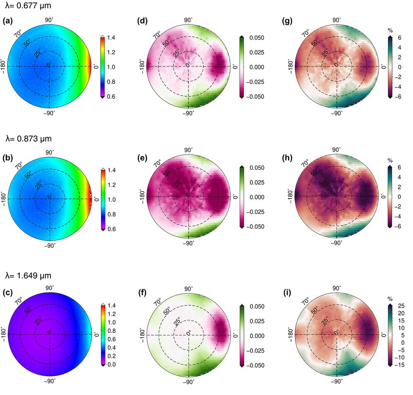
S. Jafariserajehlou et al.: Implications for the snow grain morphology in the Arctic                                            371

sition of the Troposphere from Aircraft and Satellite (ARC-         plane is defined as follows:
TAS) spring 2008 campaign over Barrow/Utqiaġvik, Alaska.
                                                                               1Lr (θi , ϕi , θr , ϕr ; λ)
Further information about the atmospheric parameters dur-           BRDFeλ =
ing the ARCTAS campaign was taken from available Aerosol                         1Ei (θi , ϕi ; λ)
Robotic Network (AERONET) and satellite data.                                   1Lr (θi , ϕi , θr , ϕr ; λ) h −1 i
                                                                             =                               sr    ,             (2)
   The paper is organized as follows: in the next section, we                  1Li (θi , ϕi ; λ) cos θi 1ωi
present the theoretical background and terminology used to
calculate the angular distribution of reflectance in a snow–        where BRDFeλ is as an average of the BRDF over an appro-
atmosphere system. In Sects. 3 and 4, we introduce and              priate area, angle, and solid angle for specific observation
explain the measurements and the simulation methods. In             geometry. 1ωi is a finite solid angle element. The validity of
Sect. 5, the sensitivity of reflectance to the underlying snow      this approximation relies on the experimental evidence that
layer and atmospheric parameters is investigated. In Sect. 6,       the BRDF is not significantly influenced by the following ef-
the results of applying the two-stage snow grain size and           fects: the finite intervals of area, angle, solid angle, and the
shape retrieval algorithm are presented. In Sect. 7, the results    distribution function, subsurface scattering, and radiation pa-
of the reflectance simulations are compared to CAR measure-         rameters such as wavelength, polarization, and fluorescence
ments. Finally, conclusions are drawn in Sect. 8. Appendix A        (i.e., significant variations do not occur within small inter-
contains a detailed description of the snow grain size and          vals; see Nicodemus et al., 1977; Gatebe and King, 2016).
shape retrieval algorithm used in the study.                        As a result, the BRDFeλ is determined by the following:
                                                                               Ler (θi , θr , 1ϕ)
                                                                    BRDFeλ =                      ,                              (3)
                                                                                  F0,λ cos θi
                                                                    where Ler is the measured radiance, and F0,λ is the solar ir-
2   Theoretical background                                          radiance incident at the top of atmosphere (TOA). Often, it
                                                                    is helpful to have a description of the difference between the
To describe the directional signature of reflectance over dif-      measured surface reflectance and a Lambertian reflector; in
ferent surface types, the bidirectional reflectance distribution    such a case, it is the equivalent bidirectional reflectance fac-
function (BRDF), as defined by Nicodemus (1965), is the             tor BRFeλ , for which BRDFeλ multiplied by π is more repre-
commonly used reflectance quantity. The term BRDF de-               sentative.
scribes the reflection of incident solar radiation from one di-        To isolate the reflectance properties of the surface and de-
rection to another direction (Nicodemus, 1965). The mathe-          rive BRFeλ or BRDFeλ just above the surface, we need to apply
matical form of BRDF is expressed as follows (Nicodemus             atmospheric-correction methods on the measured radiance at
et al., 1977; Schaepman-Strub et al., 2006):                        TOA or flight altitude (e.g., by using knowledge of the at-
                                                                    mospheric scattering or absorption by applying RTMs). This
           dLr (θi , ϕi , θr , ϕr ; λ) h −1 i                       removes the following four atmospheric contributions from
BRDFλ =                                 sr    ,              (1)    the measured radiance at TOA or flight altitude (Schaepman-
             dEi (θi , ϕi ; λ)
                                                                    Strub et al., 2006): the contribution of light scattered by the
                                                                    atmosphere (i) before the solar radiation has reached the sur-
where Lr is the reflected radiance, and θ and ϕ are the zenith      face, (ii) after being reflected by the surface, (iii) before and
and azimuth angles, respectively. The subscripts of i and r         after reaching the surface, and (iv) the atmospheric path ra-
correspond to the incident and to the reflected beams, respec-      diance.
tively. E is the incident surface flux (irradiance), and λ is the      However, most of the atmospheric contributions in mea-
wavelength. However, the BRDF is not a directly measurable          surements close to the surface are negligible (except diffuse
quantity because of its formulation as a ratio of infinites-        component number ii), and measured quantities represent the
imal quantities (Nicodemus et al., 1977; Schaepman-Strub            at-surface radiance (Schaepman-Strub et al., 2006). Sensi-
et al., 2006). Nicodemus et al. (1977) provided an exten-           tivity studies have demonstrated that atmospheric contribu-
sive description of reflectance terminologies and measurable        tions to the CAR channel observations range from 3 % to
quantities, e.g., the bidirectional reflectance factor (BRF), the   12 %, depending on the wavelength, in the range of 0.381 to
hemispherical directional reflectance factor (HDRF), the di-        2.324 µm (Soulen et al., 2000). Consequently, previous stud-
rectional hemispherical reflectance (DHR), etc. According to        ies presented either the BRFs in a surface–atmosphere sys-
Nicodemus et al. (1977) and Schaepman-Strub et al. (2006),          tem at flight altitude without atmospheric correction (Soulen
each of the terms is defined for the specific illumination and      et al., 2000) or the BRFs right above the surface after at-
reflectance geometries for which the reflectance properties         mospheric correction (Gatebe et al., 2005; Gatebe and King,
are measured (e.g., satellite, airborne, or laboratory measure-     2016).
ment conditions). Following the method of Gatebe and King              The atmospheric-correction method relies on different as-
(2016), the effective BRDF at a horizontal (flat) reference         sumptions by which several sources of uncertainty should be

https://doi.org/10.5194/amt-14-369-2021                                                  Atmos. Meas. Tech., 14, 369–389, 2021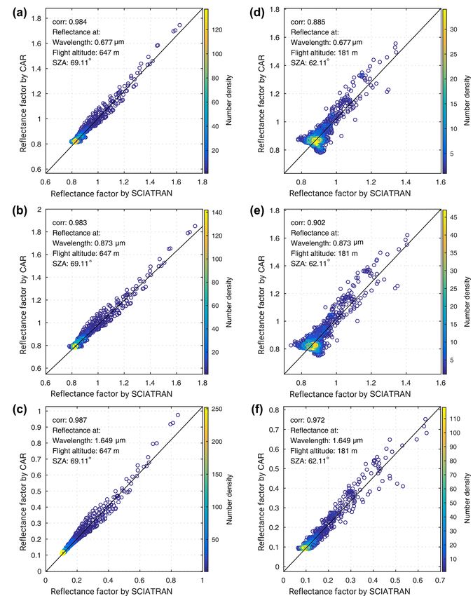
372                                     S. Jafariserajehlou et al.: Implications for the snow grain morphology in the Arctic

taken into account. In this study, to avoid such uncertainties,     ror, the instrument provides viewing geometries suitable for
we do not apply an atmospheric correction to the measure-           measurements needed for BRF calculation. CAR collects the
ments (radiances Lr, h ) at flight altitude (h). Instead, we cal-   data with a mirror rotating 360◦ in a plane perpendicular to
culate and use the reflectance at flight altitude with the fol-     the direction of flight through a 190◦ aperture that allows
lowing equation:                                                    the acquisition of data from local zenith to nadir or horizon
                                                                    to horizon with an angular resolution of 1◦ . The high angu-
       π Lr, h (θi , θr , 1ϕ)                                       lar/spatial resolution of 1◦ in both the viewing zenith and az-
R=                            ,                              (4)
           F0,λ cos θi                                              imuth angles allows the estimation of the anisotropy of the
                                                                    reflectance in the snow–atmosphere system with high accu-
where Lr, h is the measured radiance at flight altitude. All
                                                                    racy.
reflectance/BRFeλ values at flight altitude in this study repre-
                                                                       The spatial resolution of CAR depends on the flight alti-
sent R in Eq. (4) and are referred to as the reflectance factor
                                                                    tude, e.g., 10 and 18 m2 at nadir for 600 and 1000 m flight al-
in the snow–atmosphere system.
                                                                    titude, respectively, which increases with the viewing zenith
   In the simulation of the reflectance factor in a coupled
                                                                    angle (VZA), e.g., 580 m2 at 80◦ VZA for 1000 m flight al-
snow–atmosphere system, we need to account for the at-
                                                                    titude. The capability of acquiring data at different altitudes
mospheric effects contribution properly. For this reason, we
                                                                    (∼ 200, 600, and 1700 m) enables us to evaluate the sensitiv-
take independent data about atmospheric parameters (aerosol
                                                                    ity of reflectance with respect to atmospheric effects in RTM
optical thickness, AOT, and gases absorption) from ground-
                                                                    simulations.
based and space-borne measurements. We select the data
                                                                       Examples of calculated reflectance factor values using
with the closest spatial and temporal interval actual airborne
                                                                    Eq. (4) from CAR measurements on 7 April 2008 at Elson
measurements. We discuss more details of the atmospheric
                                                                    Lagoon (71.3◦ N, 156.4◦ W) are shown in Figs. 2 and 3. As
data and their application to the simulation routine in Sects. 3
                                                                    we can see in these two figures, in spite of the influence of
and 4. To estimate BRFeλ just above the surface, further atmo-
                                                                    the atmospheric scattering and absorption, the general fea-
spheric correction is needed. We assume the reflectance fac-
                                                                    tures of the snow BRF are clearly observable in polar plots
tor at flight altitude is a good estimation of BRFeλ just above
                                                                    and principal and cross-plane plots because of (i) the de-
the surface at infrared wavelengths where atmospheric scat-
                                                                    crease in snow reflectance with increasing wavelength due
tering is negligible.
                                                                    to the increasing absorption by snow at longer wavelengths,
                                                                    (ii) the increase in the snow BRF as a function of VZA and
3     Measurements                                                  the strong forward-scattering peak in the principal plane at
                                                                    large VZA, and (iii) the smaller angular variation in the BRF
CAR is an airborne instrument developed at NASA’s God-              at cross plane compared to the principal plane, though the re-
dard Space Flight Center. It has been used during several field     flectance values increase with VZA. The snow surface spatial
campaigns around the world from 1984 up to the present.             inhomogeneity decreases with increasing altitude due to the
CAR has been used to measure the single scattering albedo of        change in spatial resolution with altitude (Gatebe and King,
clouds, the bidirectional reflectance of various surface types,     2016; Lyapustin et al., 2010). Accordingly, at poorer spa-
and for acquiring imagery of clouds and the Earth’s surface.        tial resolutions, spatial homogeneity is more efficiently av-
For this study, we used CAR data from the ARCTAS cam-               eraged, as can be seen in Fig. 2 at flight altitude of 1700 m,
paign conducted at Elson Lagoon, near Barrow/Utqiaġvik,            compared to 206 m, in which we have a higher spatial reso-
Alaska, in April 2008 as part of the International Polar Year       lution.
(Lyapustin et al., 2010; Gatebe and King, 2016). The goal              To account for aerosols, we use the aerosol optical thick-
of ARCTAS was to study physical and chemical processes              ness (AOT) data acquired by the nearby Aerosol Robotic
in the Arctic atmosphere and (e.g., long-range transport of         Network (AERONET) sun photometer at Barrow/Utqiaġvik
pollution to the Arctic) and surface parameters (e.g., snow         during the CAR measurement time. AERONET is a glob-
reflectance angular variation). A P-3B aircraft carried the         ally distributed network and provides long-term and continu-
CAR instrument and was deployed by NASA from Fair-                  ous ground-based measurements of the total column aerosol
banks, Alaska. Figure 1 shows the flight track on 7 April           optical thickness derived from the attenuation of sunlight.
2008. The date, location, measurement geometry, and avail-          The data are provided often at a high temporal resolution
able atmospheric parameters during the measurements used            of 15 min. AERONET AOT data are provided at 0.5 and
in this study are presented in Table 1.                             0.6 µm wavelengths. We use the Ångström exponent to cal-
   The unique design of CAR simultaneously provides both            culate AOT values at the reference wavelength (0.55 µm) re-
up-welling and down-welling radiances at 14 spectral bands          quired for the SCIATRAN simulation. Table 1 shows the
(Table 2) located in the atmospheric window regions of UV,          calculated AOT at 0.55 µm, based on AERONET data for
visible, and near-infrared from 0.34 to 2.3 µm, comprising          Barrow/Utqiaġvik at the closest time to the CAR airborne
important wavelengths relevant for remote sensing applica-          measurements. The aerosol condition and its chemical and
tions such as aerosol retrievals. Through a rotating scan mir-      optical properties have been measured continuously at Bar-

Atmos. Meas. Tech., 14, 369–389, 2021                                                 https://doi.org/10.5194/amt-14-369-2021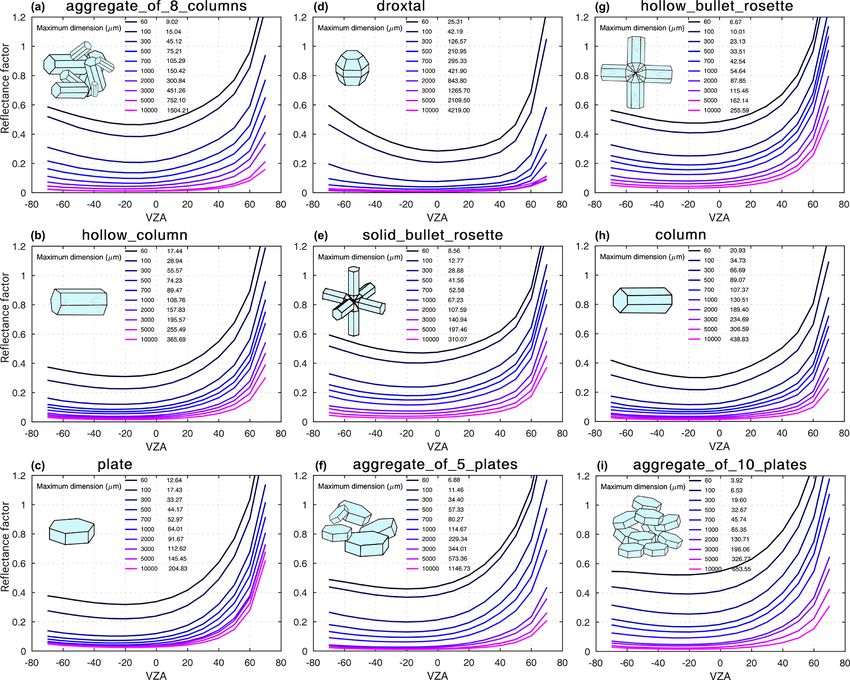
S. Jafariserajehlou et al.: Implications for the snow grain morphology in the Arctic                                              373

Figure 1. Flight track of P-3B airplane carrying NASA’s Cloud Absorption Radiometer (CAR) on 7 April 2008 during the Arctic Research
of the Composition of the Troposphere from Aircraft and Satellite (ARCTAS) campaign (figure adapted from: https://www-air.larc.nasa.
gov/missions/arctas/arctas.html, last access: November 2020). Image credits: © NASA; © Tele Atlas 2008; © Europa Technologies 2008;
© TerraMetrics 2008; © 2007 Google.

Table 1. Summary of the CAR, Aerosol Robotic Network (AERONET) aerosol optical thickness (transferred from 0.5 to 0.55 µm), and
weighting function differential optical absorption spectroscopy (WFDOAS) ozone data used in this study. Note: solar zenith angle – SZA.

                        Data set number       1                2                3               4
                        Date                  7 April 2008     7 April 2008     7 April 2008    15 April 2008
                        Location              Elson Lagoon     Elson Lagoon     Elson Lagoon    Elson Lagoon
                        Flight altitude       206 m            647 m            1700 m          181 m
                        SZA (θ0 )             70.23◦           69.11◦           67.78◦          62.11◦
                        AOT (τ 0.55 µm)       0.11             0.11             0.11            0.15
                        Total ozone column    416 DU           416 DU           416 DU          463.4 DU

row, Alaska, during different seasonal periods (Quinn et              set (covering 1995 to the present) consists of merged total
al., 2002). Previous studies indicate the largest contribution        ozone column data retrieved by WFDOAS from the Global
from sea salt, non-sea-salt sulfate, and mineral dust. The av-        Ozone Monitoring Experiment (GOME), Scanning Imag-
erage contribution of black carbon is very small compared             ing Absorption Spectrometer for Atmospheric Chartography
to other aerosol types (Udisti et al., 2020). During the haze         (SCIAMACHY), and GOME-2A. In this paper, the ozone to-
season (January to April), sea salt plays the dominant role in        tal column data are selected using the criteria of having the
controlling light scattering in wintertime and non-sea salt sul-      smallest temporal and spatial differences with CAR data. For
fate in spring (Quinn et al., 2002). The increase in non-sea-         nitrogen dioxide, we use vertical column information from
salt (nss) sulfate in January to May is the long-range transport      the SCIATRAN database obtained from a 2D chemical trans-
of anthropogenic primary nss sulfate, besides the long-range          port model developed at the University of Bremen (Sinnhu-
transport of anthropogenic SO2 and its photo-oxidization to           ber et al., 2009).
nss sulfate with the increase of light levels, and the local pro-        The derived AOT and trace vertical column have been used
duction of biogenic nss sulfate.                                      in the simulation of radiative transfer processes in the snow–
   To account for ozone absorption, we use knowledge of the           atmosphere system.
ozone total column amount retrieved from the space-borne
measurements by using the University of Bremen weighting
function differential optical absorption spectroscopy (WF-
DOAS) algorithm version 4 (Weber et al., 2018). This data

https://doi.org/10.5194/amt-14-369-2021                                                    Atmos. Meas. Tech., 14, 369–389, 2021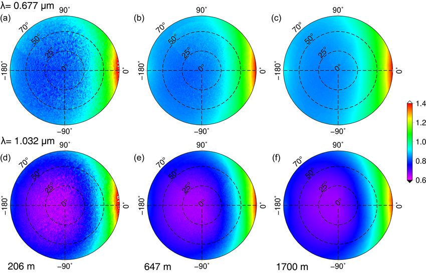
374                                        S. Jafariserajehlou et al.: Implications for the snow grain morphology in the Arctic

Figure 2. Angular distribution of reflectance factor in the snow–atmosphere system derived from CAR measurements on 7 April 2008 at
Elson Lagoon (71.3◦ N, 156.4◦ W), showing reflectance at the 0.677 µm wavelength and three flight altitudes of 206, 647, and 1700 m,
respectively (a, b, c), and the 1.032 µm wavelength and the same flight altitudes (d, e, f). The principal plane is the horizontal line (ϕ = 0 and
180◦ ), and the viewing zenith angle is shown as the radius of the polar plots from 0◦ (nadir) to 70◦ . The solar zenith angle is 70.23, 69.11,
and 67.78◦ for flight altitudes of 206, 647, and 1700 m, respectively.

Figure 3. Angular distribution of the reflectance factor in the snow–atmosphere system, derived from measurements by CAR at 647 m flight
altitude and six wavelengths of 0.677, 0.873, 1.032, 1.222, 1.275, and 1.649 µm on 7 April 2008 at Elson Lagoon (71.3◦ N, 156.4◦ W).
(a) The principal plane (ϕ = 0 and 180◦ ) and (b) cross plane (ϕ = 90 and 270◦ ).

4     Simulations                                                          assuming either a plane parallel or a spherical atmosphere
                                                                           (Rozanov et al., 2014).
                                                                              In this paper, to calculate the reflectance factor values,
SCIATRAN is a software package for radiative trans-
                                                                           SCIATRAN assumes that the snow is a layer with an optical
fer modeling developed at the Institute of Environmental
                                                                           thickness of 1000 and a geometrical thickness of 1 m, com-
Physics (IUP), University of Bremen (Rozanov et al., 2002,
                                                                           posed of ice crystals of different morphologies and placed
2014), and freely available at http://www.iup.uni-bremen.de/
                                                                           above a black surface. This assumption was successfully val-
sciatran/ (last access: February 2020). The SCIATRAN pack-
                                                                           idated by Rozanov et al. (2014). The snow layer is assumed
age has been used in a variety of remote sensing studies to
                                                                           to be vertically and horizontally homogeneous and composed
simulate radiative transfer processes in a wide spectral range,
                                                                           of a monodisperse population of ice crystals. The impact of
from the ultraviolet to the thermal infrared (0.18–40 µm),

Atmos. Meas. Tech., 14, 369–389, 2021                                                           https://doi.org/10.5194/amt-14-369-2021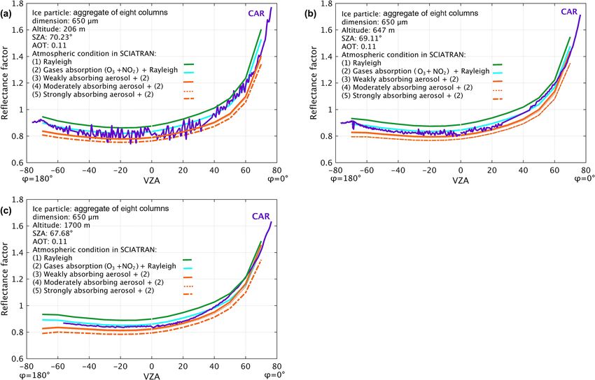
S. Jafariserajehlou et al.: Implications for the snow grain morphology in the Arctic                                             375

Table 2. Summary of CAR wavelengths and bandwidth.                   ing the modified single scattering properties of sparsely dis-
                                                                     tributed particles, as suggested in Mishchenko (1994). The
      Channel number     Central wavelengths     Bandwidth           comparison of snow BRFs calculated assuming sparsely or
                                 (µm)                (nm)            densely packed snow layers shows that the maximum dif-
      1                         0.480                    21          ference does not exceed 0.015 % (Pohl et al., 2020). There-
      2                         0.687                    26          fore, this effect was ignored in radiative transfer calculations
      3                         0.340                     9          through the snow layer.
      4                         0.381                     6             To account for atmospheric effects, SCIATRAN incor-
      5                         0.870                    10          porates a comprehensive database containing monthly and
      6                         1.028                     4          zonal vertical distributions of trace gases, e.g., O3 , NO2 ,
      7                         0.609                     9          SO2 , H2 O, etc., spectral characteristics of gaseous absorbers,
      8                         1.275                    24          vertical profiles of pressure and temperature, and molec-
      9                         1.554                    33          ular scattering characteristics (see Rozanov et al., 2014,
      10                        1.644                    46
                                                                     for details). To account for scattering and absorption by
      11                        1.713                    46
      12                        2.116                    43
                                                                     aerosols over snow in SCIATRAN, the optical characteristics
      13                        2.203                    43          of aerosol particles and vertical distribution of aerosol num-
      14                        2.324                    48          ber density are required. In this study, we use Moderate Res-
                                                                     olution Imaging Spectrometer (MODIS) collection 5 aerosol
                                                                     parameterization (Levy et al., 2007) as an internal database
                                                                     in SCIATRAN. Levy et al. (2007) developed a framework for
impurities in the snow (e.g., black carbon) is neglected in          connecting the aerosol microphysical properties, such as the
this study. To simulate the radiative transfer through a snow        refractive index and size distribution to the AOT at 0.55 µm.
layer, the single scattering properties of ice crystals, includ-     Using AOT from ground-based measurements of AERONET
ing extinction and scattering efficiencies, single scattering        at Barrow/Utqiaġvik, as mentioned, and selecting one of the
albedo, and phase functions, need to be defined in SCIA-             aerosol types, the Mie code incorporated into SCIATRAN is
TRAN. All these parameters are dependent on the wave-                employed to calculate aerosol extinction and scattering coef-
length, size, and shape of the particle (Leroux et al., 1999).       ficients. In this study, the vertical profile of aerosol number
Recently, a new data library of basic single scattering prop-        density, as an exponential vertical distribution for a height of
erties of nine ice crystal shapes/habits developed by Yang et        3.0 km, is used.
al. (2013) has been incorporated in the SCIATRAN model                  For the conditions described above, the radiative transfer
(Pohl et al., 2020). This database comprises a full set of           calculations are performed at a source–target–sensor geome-
single scattering properties at wavelengths from the UV to           try extracted from the airborne measurements at solar zenith
the far infrared (IR) for the following nine ice crystal mor-        angles of 70.23, 69.11, 67.68, and 62.11◦ together with a
phologies: droxtal, column and hollow column, aggregate of           viewing zenith angle (0–70◦ ) and relative azimuth angle (0–
eight columns, plates, small aggregate of five plates, large         360◦ ), with an angular resolution of 5◦ , and at four differ-
aggregate of 10 plates, and hollow and solid bullet rosettes.        ent altitudes of 181, 206, 647, and 1700 m. More detailed in-
More detailed information about the ice crystal shapes and           formation about atmospheric and snow layer parameters are
sizes can be found in Yang et al. (2013). In addition to the         given and discussed separately in the following section.
abovementioned nine ice crystals, optical parameters for tri-
adic Koch fractal (referred to as fractal in this paper) particles
are used as well (Macke et al., 1996; Rozanov et al., 2014).         5   Sensitivity of reflectance to the snow morphology and
The fractal particle model uses regular tetrahedrons as its              atmospheric parameters
basic elements. In this study, we use the second-generation
fractals, as described in Macke et al. (1996) and Rozanov et         The measured reflectance in the visible and near infrared
al. (2014).                                                          (NIR) spectral range over a snow field depends on the rel-
   In SCIATRAN, the snow grains are specified by their               ative importance of the absorption and scattering radiative
single scattering properties of sparsely distributed particles.      transfer processes in the atmosphere and snow layer. In this
Namely, the snow grains are assumed to be in the far field           section, we investigate the sensitivity of the reflectance on
zones of each other and will thus scatter the light indepen-         the radiative transfer through the atmosphere and the snow at
dently. For a snow layer, the snow grains can be located             the selected wavelength bands (i) 1.649 µm, because of the
in each other’s near field, resulting in interactions between        high sensitivity of this wavelength to snow grain properties,
the scattered electromagnetic fields of neighboring particles        and (ii) 0.677 and 0.873 µm wavelengths, because of the rel-
which lead to the modification of single scattering properties       atively high and differing sensitivities at these wavelengths
(Mishchenko, 2014; Mishchenko, 1994). The impact of the              to the atmospheric conditions being used for aerosol optical
near-field effect was investigated in Pohl et al. (2020), us-        thickness retrievals.

https://doi.org/10.5194/amt-14-369-2021                                                  Atmos. Meas. Tech., 14, 369–389, 2021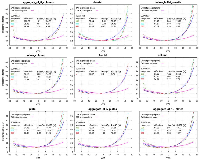
376                                     S. Jafariserajehlou et al.: Implications for the snow grain morphology in the Arctic

Figure 4. The change in reflectance factor values in the principal plane (ϕ = 0 and 180) with the size and shape of ice crystals at the
wavelength of 1.649 µm. The left column of the legend in each panel shows the maximum length of the ice crystal, and the right column is
its equivalent effective radius.

5.1   Impact of snow: size and shape of ice crystals                    ii. The BRF properties of snow at 1.649 µm are closer to
                                                                            those for single scattering behavior, and this is linked to
To study the influence of ice crystal morphology on the ra-                 the phase function, which strongly depends on the shape
diation field above snow-covered surfaces, we perform the                   of ice crystals.
simulation at 1.649 µm for the following three important rea-          iii. The impact of the atmosphere (absorption by CO2 and
sons (Leroux et al., 1998):                                                 H2 O and diffuse incident irradiance) at 1.649 µm is neg-
                                                                            ligible.
  i. The absorption of ice crystals is small or negligible at            To illustrate the high sensitivity of the radiation field to
     the selected wavelengths in the visible domain of the            the varying sizes of ice crystals at 1.649 µm, we simulated
     spectrum. In contrast, in the near-infrared range, due           the snow reflectance factor at principal and cross planes,
     to the large absorption of ice crystals at these wave-           assuming nine ice crystal morphologies with varying sizes
     lengths, the snow reflectance is significantly affected by       (here size refers to maximum dimension/edge length), 60 ∼
     the snow grain size – the larger the particle, the smaller       10 000 µm, and three different roughnesses (smooth surface –
     the reflectance because of larger absorption and stronger        0; moderate surface roughness – 0.03; severe surface rough-
     forward scattering.                                              ness – 0.50). For further information, see Yang et al. (2013).

Atmos. Meas. Tech., 14, 369–389, 2021                                                    https://doi.org/10.5194/amt-14-369-2021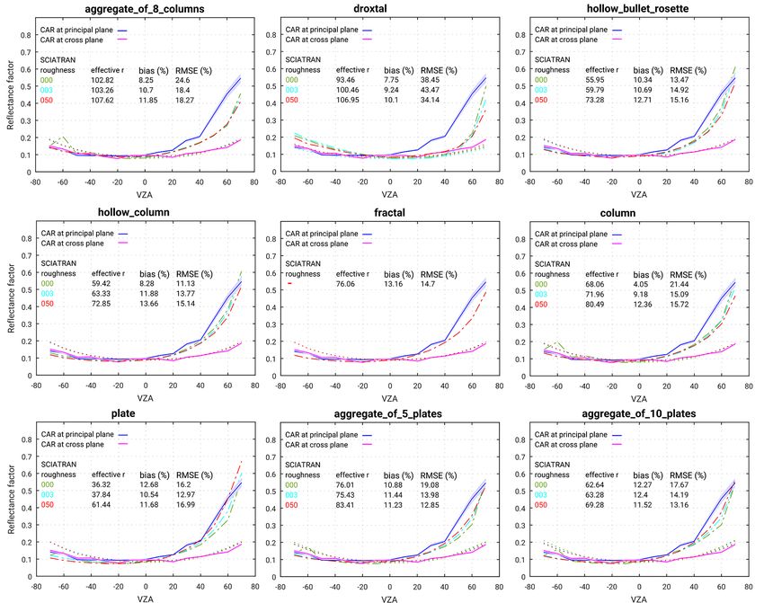
S. Jafariserajehlou et al.: Implications for the snow grain morphology in the Arctic                                            377

Figure 4 shows the simulated reflectance factor versus the           we assume an atmosphere over the snow layer, which con-
VZA in the principal plane (as the most sensitive and repre-         tains (i) Rayleigh scattering (scattering by air molecules),
sentative direction for the largest changes of reflectance) us-      (ii) gaseous absorption, and (iii) absorption and scattering by
ing severely roughened morphology. As can be seen in Fig. 4,         aerosols. Therefore, in this section, absorption bands, e.g.,
the reflectance factor strongly changes with the size of ice         0.677 µm are selected to evaluate the impact of the atmo-
crystals from 60 to 10 000 µm. The equivalent effective ra-          sphere. We calculate the reflectance factor at 0.677 µm un-
dius1 is shown beside the maximum lengths of ice crystals in         der three different conditions, assuming a model atmosphere
Fig. 4. Differentiating between various shapes has the largest       governed, (i) by Rayleigh scattering, (ii) identical to (i) but
effect in the forward-scattering (ϕ = 0◦ ) and a lesser effect       with absorption by ozone (O3 ) and nitrogen dioxide (NO2 ),
in backward-scattering direction (ϕ = 180◦ ). The results in-        and (iii) identical to (ii) but including aerosol. The calcula-
dicate that the effect of changing size is larger than the im-       tions are performed assuming the following properties of the
pact of differentiating between various shapes of ice crystals       atmosphere and snow layer:
at this wavelength.
   Using the aggregate of eight columns shape and changing             i. Vertical profile of nitrogen dioxide, pressure, and tem-
the maximum dimension from 60 to 10 000 µm results in a                   perature are selected according to a 2D chemical trans-
reflectance decrease of ∼ 40 % at the nadir (VZA ∼ 0◦ ) and               port model (Sinnhuber et al., 2009) incorporated in SCI-
more than 80 % in the forward-scattering direction (at VZA                ATRAN.
of 60◦ ), which is considerably large. If we change only the
shape of the snow grain from an aggregate of eight columns            ii. Total vertical column of ozone and AOT are set accord-
to the droxtal, but we keep the size (largest dimension) as it            ing to Table 1.
is (e.g., 300 µm), this change provides a noticeable decrease
of ∼ 30 % in reflectance at the forward-scattering direction          iii. Snow layer is composed of ice crystals having the shape
for a viewing zenith angle of 60◦ , and this leads to a much               aggregate of eight columns, a maximum dimension of
weaker forward peak. What is noteworthy is that the plate                  650 µm, and a severely roughened crystal surface.
shape cannot reproduce the enhancement in a backward di-
rection (typical for a BRF over snow) that is as strong as what         Figure 5 shows the impact of the atmosphere and the dif-
the aggregate of eight columns or the droxtal shape causes.          ference between measured and simulated reflectance factor
Using the aggregate of five and 10 plates leads to larger re-        values at three different altitudes (206, 647, and 1700 m) for
flectance in all directions compared to the single plate shape.      the three scenarios. The reflectance reduction at 647 m flight
However, the analysis of the simulation results at the cross         altitude due to gaseous absorption is the smallest (∼ 5 %)
plane (not shown here) indicates that the impact on the re-          close to the nadir region and becomes larger (∼ 10 %) in the
flectance pattern, originating from the specific shapes of the       forward-scattering direction, which decreases (to ∼ 8 %) at
ice crystals, is relatively small compared to the impacts at the     1700 m altitude. At this wavelength, ozone with a vertical
principal plane.                                                     optical depth (VOD) of 1.6 × 10⁻² has a much larger contri-
   The large range of changes in the reflectance in both the         bution to gaseous absorption compared to that of NO2 with a
principal and cross planes, when using different ice crystal         VOD of 3.95 × 10⁻⁵ .
morphologies, highlights the importance of having accurate              The reflectance for an atmosphere containing three types
a priori knowledge or estimations of the size and shapes of          of aerosol (weakly, moderately, or strongly absorbing
the ice crystals to accurately reproduce measurements. In our        aerosol) and without aerosol (containing only Rayleigh and
study, due to the lack of such information from in situ mea-         gaseous absorption) is presented in Fig. 5. For more infor-
surements, we estimate the size of ice crystals for each se-         mation on the aerosol typing used in this study see Levy et
lected crystal shape separately to have a priori knowledge of        al. (2007). The changes in reflectance, due to weakly absorb-
ice crystal properties and to limit the differences between the      ing aerosol with an AOT of 0.11 (measured by AERONET) at
simulated and measured reflectance. The detailed explana-            206 m flight altitude, are ∼ 5 % at the nadir and an increase
tion and results are given in Sect. 6.                               in the forward-scattering direction to ∼ 13 %. The strongly
                                                                     absorbing aerosol (at the same AOT of 0.11) reduces the re-
5.2   Impact of atmosphere: scattering and absorption                flectance by ∼ 7 % at the nadir and ∼ 20 % in the forward-
      by aerosol and gases                                           scattering direction. At 1700 m, the reflectance decreases by
                                                                     6 % at the nadir and 7 % in the forward-scattering direction.
The incident radiation is composed of direct sunlight and            The differences between the three aerosol types does not lead
the diffuse radiation from the sky (Aoki et al., 1999). To           to changes in reflectance which are larger than 5 % in or
take the atmospheric absorption and scattering into account,         close to nadir areas. In summary, an atmosphere containing
   1 Effective radius = 3/4×(V /A ), where V is total volume,
                               tot tot           tot                 Rayleigh scattering, absorption by ozone (O3 ) and nitrogen
and Atot is the total projected area of ice per unit volume of air   dioxide (NO2 ), and weakly absorbing aerosol is the best rep-
(Baum et al., 2014).                                                 resentation of the atmospheric conditions for our case study.

https://doi.org/10.5194/amt-14-369-2021                                                  Atmos. Meas. Tech., 14, 369–389, 2021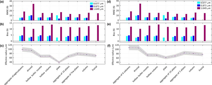
378                                         S. Jafariserajehlou et al.: Implications for the snow grain morphology in the Arctic

Figure 5. Measured and simulated reflectance factor at 0.677 µm versus the viewing zenith angle (VZA) in the principal plane (ϕ = 0 and
180◦ ) at three different flight altitudes. Panels represent results at 206, 647, and 1700 m flight altitudes, respectively. The green lines indicate
simulated reflectance assuming Rayleigh scattering (case i). The blue line shows reflectance for case ii (as in case i, including absorption of
O3 and NO2 ). The orange lines show the reflectance for case iii (as in case ii but adding aerosol with an aerosol optical thickness (AOT) of
0.11 for three types of aerosol, namely (i) weakly absorbing, (ii) moderately absorbing, and (iii) strongly absorbing).

6   Retrieval of snow grain size and shape                                   and cross planes. The absolute uncertainty of CAR measure-
                                                                             ments is within 5 % and is shown by the uncertainty envelope
In the previous section, we showed that having adequate a                    (shading). The accuracy of our radiative transfer calculations
priori information about the snow surface and atmosphere is                  is estimated to be in the range of 0.1 %. Based on the compar-
necessary for calculating the reflectance factor with sufficient             ison, one can state that the angular reflectance pattern of the
accuracy. In contrast to the atmospheric parameters available                CAR measurement on 7 April 2008 at Elson Lagoon is re-
from independent sensors and models, a priori knowledge                      produced by SCIATRAN successfully. The highest accuracy
about ice crystal size and shape for the underlying snow layer               is obtained by assuming ice crystals as an aggregate of eight
is not typically available. To estimate the optimal ice crystal              columns with severely roughened crystal surface at an effec-
morphology, we used a snow grain size- and shape-retrieval                   tive radius of 98.8 µm (corresponding to a maximum dimen-
algorithm by minimizing the difference between the mea-                      sion of 650 µm). In this case, the largest and smallest discrep-
sured and simulated reflectance factor (see Appendix A for                   ancies appear in the forward-scattering direction and close
details). Here, size refers to the effective radius of the ice               to the nadir (VZA < ±25◦ ), respectively. The overall RMSE
crystal. The retrieval algorithm is applied to measurements                  and bias between measurements and simulation at the prin-
at principal and cross planes at 1.649 µm, assuming different                cipal plane is 6.9 % and 2.7 %, respectively. A lesser degree
shape and crystal surface roughnesses. To find the best rep-                 of agreement between simulated results and measurements is
resentative shape and size, the bias and root mean square er-                provided by using column and fractal shapes with an RMSE
ror (RMSE) between the measured and simulated reflectance                    of 7.3 % and 9.75 %, respectively. The largest difference be-
factor were determined for each case study.                                  tween measurements and simulations is observed for the case
   Figure 6 shows one example of the comparison between                      using the droxtal shape with an RMSE ∼ 25.54 %.
the measured and simulated reflectance factor at principal

Atmos. Meas. Tech., 14, 369–389, 2021                                                             https://doi.org/10.5194/amt-14-369-2021
S. Jafariserajehlou et al.: Implications for the snow grain morphology in the Arctic 379 Figure 6. Comparison of measured and simulated reflectance factors. Measurements were performed by the CAR instrument over old snow at 647 m flight altitude on 7 April 2008 at 1.649 µm. The uncertainty in CAR measurements is indicated by the envelope (shading). SCIATRAN simulations in the principal and cross plane given by the dashed–dotted and dotted lines, respectively, and by different colors (green, blue, and red) present smooth, moderately roughened, and severely roughened crystal surfaces. Positive and negative VZAs correspond to azimuthal angles ϕ = 0 and 180◦ for the principal plane and ϕ = 90 and 270◦ for the perpendicular plane, respectively. We also retrieved the effective radius of ice crystal using ∼ 13.16 % and 14.69 %, respectively. The results obtained CAR data for fresh fallen snow on 15 April 2008. Due to by using the droxtal ice crystal shape exhibit large differ- the existing surface horizontal inhomogeneity for the case of ences in both of forward- and backward-scattering directions fresh snow acquired at a lower flight altitude ∼ 181 m, larger with an RMSE of 34.1 %. differences between simulated and measured reflectance are Though the real nature of the ice crystal shape at the time expected, compared to the old snow case on 7 April 2008. of measurement is not known to us, the impact of tempera- The results are shown in Fig. 7. Unlike the old snow case ture and supersaturation on the morphology of snow grain presented in Fig. 6, the aggregate of eight columns shape particles has been debated in previous studies (Slater and does not optimally represent the ice crystals of this particu- Michaelides, 2019; Shultz, 2018; Libbrecht, 2007; Bailey lar day. Rather, a reflectance simulated by using an aggregate and Hallett, 2004; Yang et al., 2003). Based on the relation- of five plates as the ice crystal shape provides the minimum ship between temperature and snow grain morphology, the RMSE ∼ 12.85 % between the measurement and simulation column-based shapes are the dominant ice crystal morphol- results. An aggregate of 10 plates and fractal provide the sec- ogy in environments with temperatures higher than −10 ◦ C, ond and third most representative shapes, with an RMSE of whereas plates are dominant if the temperature is less than https://doi.org/10.5194/amt-14-369-2021 Atmos. Meas. Tech., 14, 369–389, 2021
380                                     S. Jafariserajehlou et al.: Implications for the snow grain morphology in the Arctic

Figure 7. The same as Fig. 6 but the measurements by the CAR instrument were performed on 15 April at 181 m flight altitude over fresh
snow.

−10 ◦ C. Though more investigation is needed, especially             CAR measurements in any of our scenarios. With respect to
to account for the temperature profile at the exact time of          the size of ice crystals, we do not compare fresh and old snow
snowfall, our findings with respect to the most representative       cases because it is important to note that the date of the old
shape for each case study agree with this argument. The tem-         snow case is before fresh snow. This means the studied old
perature range during CAR measurements on 6–7 April 2008             snow case is not the aged fresh snow case. Therefore, the
is from −20 to −5 ◦ C. Based on our results, the aggregate of        change in ice crystal size with its age is not studied in the
eight columns is the most representative shape for measure-          scope of this paper.
ments conducted on this day. On 15 April 2008, when the                 A summary of retrieved effective radii using different ice
temperature range changes to −23 to −17 ◦ C, mainly plate-           crystal shapes and corresponding bias and RMSE values is
based ice crystal shapes are expected for such low tempera-          presented in Table 3. The ice crystals with a minimum RMSE
tures, and our results confirm this argument. In addition, the       value at 1.649 µm are italicized and selected to be used for
existence of droxtal ice crystals during the measurement is          subsequent calculations of the reflectance factor at 0.677 and
less probable because very low temperatures (∼ −50 ◦ C) are          0.873 µm. In Fig. 8, the importance of the ice crystal shape
needed to form droxtal or quasi-spherical ice crystals (Yang         selection for the snow grain size retrieval and the snow re-
et al., 2003). The temperature dependence of the ice crystal         flectance calculation is highlighted. The measurements were
morphologies explains, in part, why droxtal-shaped ice crys-         selected from the old snow and fresh snow cases. The effec-
tals do not capture the derived snow reflectance values from         tive radius is retrieved only at 1.649 µm, and then it is used

Atmos. Meas. Tech., 14, 369–389, 2021                                                   https://doi.org/10.5194/amt-14-369-2021
S. Jafariserajehlou et al.: Implications for the snow grain morphology in the Arctic 381
Table 3. Retrieval of the physical characteristics of ice crystals with different shapes in the case of most roughened habits. Numbers in italics
indicate minimum root mean square error (RMSE).
Ice crystal habit Asymmetry parameter Retrieved effective Old snow Fresh snow
radius (µm)
Old Fresh Old Fresh Bias RMSE Bias RMSE
snow snow snow snow (%) (%) (%) (%)
Fractal 0.825 0.827 69.37 76.06 3.50 9.75 13.16 14.69
Droxtal 0.856 0.863 94.48 106.95 0.87 25.54 10.10 34.14
Column 0.873 0.877 74.71 80.49 2.17 7.32 12.36 15.72
Hollow column 0.884 0.888 67.32 72.85 2.80 11.15 13.66 15.14
Aggregate of eight columns 0.844 0.849 98.83 107.62 2.79 6.97 11.85 18.27
Plate 0.923 0.942 38.93 61.44 −0.44 21.47 11.68 16.99
Aggregate of five plates 0.874 0.877 78.02 83.41 1.82 10.34 11.23 12.85
Aggregate of 10 plates 0.893 0.893 65.36 69.28 2.34 13.91 11.52 13.16
Hollow bullet rosette 0.887 0.889 67.01 73.28 2.16 9.99 12.71 15.16
Figure 8. Comparison of snow grain size retrieval and best fit of reflectance at three wavelengths of 0.677, 0.873, and 1.649 µm. (a, b, c) Old
snow case and (d, e, f) fresh snow case. Effective radius is retrieved at 1.649 µm, and the gray envelope (shading) shows the uncertainty in
the retrieved effective radius.
to calculate the reflectance factor at 0.677 and 0.873 µm. The directions is smaller than what is presented here. It can be
results are presented in Fig. 8, with the corresponding RMSE seen that the RMSE values at 0.677 and 0.873 µm are sig-
and bias values in the principal plane. The uncertainty of the nificantly smaller than that at 1.649 µm. This is explained by
effective radius retrieval is estimated to be ∼ 10 %, on the the high reflectance values at these wavelengths, and there-
basis of the optimal estimation technique, and is shown by fore the larger denominator in RMSE formula, in which the
the gray envelope (shading) in Fig. 8. It can be seen that difference of measured and simulated reflectance factor is di-
the retrieved effective radius value changes from shape to vided by the measured reflectance.
shape. The difference in retrieved effective radius generally
does not exceed 40 %, but in the case of the plate ice crys-
tals, the retrieved effective radius is ∼ 70 % smaller than the 7 Comparison of measured and simulated reflectance
other shapes, e.g., the aggregate of eight columns. This is a factor
significantly large difference. However, these results are pre-
In this section, we present the results of the comparison of
sented for the principal plane in which the maximum dif-
the measured and simulated reflectance factor in the snow–
ferences between simulation and measurement are expected.
atmosphere system. The simulations, which used the results
Therefore, the overall bias and RMSE value on all azimuth
and findings described in the previous section, were per-
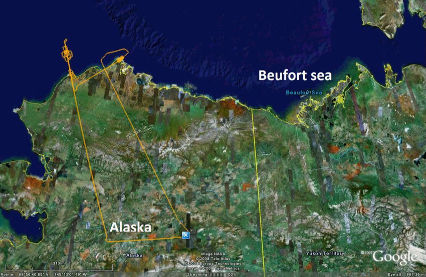
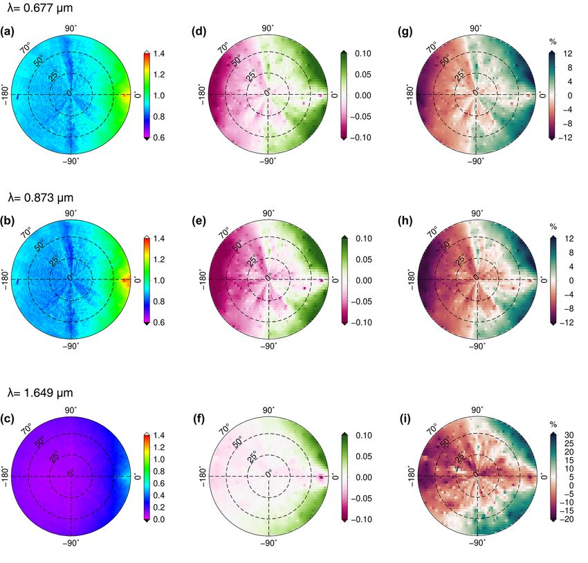
https://doi.org/10.5194/amt-14-369-2021 Atmos. Meas. Tech., 14, 369–389, 2021382 S. Jafariserajehlou et al.: Implications for the snow grain morphology in the Arctic Figure 9. (a, b, c) The reflectance factor at three wavelengths, namely 0.677, 0.873, and 1.649 µm, from the CAR measurements acquired on 7 April 2008 at Barrow/Utqiaġvik, Alaska, at an altitude of 647 m. (d, e, f) The absolute difference between reflectance of simulation (RSCIATRAN) and that of measurement (RCAR): (RSCIATRAN − RCAR). (g, h, i) The relative difference in percent (%). formed by assuming an atmosphere containing O3 , NO2 , and ±0.05 for small VZA. The difference between SCIATRAN weakly absorbing aerosol, as described in Table 1. The snow simulation values and those of the measurements is pro- layer is assumed to be comprised of an aggregate of eight col- nounced in the forward-scattering region where |1ϕ| < 40◦ . umn ice crystals, with a maximum dimension of 650 µm (ef- Figure 10 is the same plot as Fig. 9 but for fresh snow. The fective radius 99 µm) for the case of the old snow, and an differences between the SCIATRAN simulations and CAR aggregate of five plates ice crystals, with a maximum dimen- measurements of the reflectance factor are less pronounced sion of 725 µm (effective radius 83 µm) for the case of the in the glint region, compared to those for the old snow. fresh snow. To assess the accuracy of the simulations over all azimuth In Fig. 9, the difference between the simulated and mea- angles, the correlation plot and the Pearson correlation coef- sured reflectance factor at 0.677 and 1.649 µm is small on ficient between the measured and modeled reflectance factor average, being less than 0.025 in regions of small VZA and are shown in Fig. 11. As it is shown in Fig. 11, the correla- not exceeding ±0.05 for larger VZA < 50◦ . These values tion coefficient between reflectance measurements over old are larger at 0.873 µm; the maximum difference reaches ∼ snow and simulation is high, ∼ 0.98. We consider that sur- Atmos. Meas. Tech., 14, 369–389, 2021 https://doi.org/10.5194/amt-14-369-2021
S. Jafariserajehlou et al.: Implications for the snow grain morphology in the Arctic                                              383

Figure 10. The same as Fig. 9 but the measurements by the CAR instrument were performed on 15 April 2008 at 181 m flight altitude over
fresh snow.

face inhomogeneities and related larger shadowing effects at         8   Conclusion
a measurement altitude of 181 m explain why the correla-
tion decreased to 0.88 at 0.677 µm (for the case of old snow,        In this study, our objective was to assess the accuracy of the
acquired at 647 m flight altitude, surface inhomogeneities are       simulation of the reflectance in a snow–atmosphere system,
smoothed, and therefore, the old snow case is less affected by       taking different snow morphology and atmospheric absorp-
surface inhomogeneities). However, in Fig. 11, at 1.649 µm           tion and scattering into account. For this, we used a state-of-
the correlation coefficient is high ∼ 0.97 for the case of fresh     the-art RTM, SCIATRAN, which used explicit models of the
snow, possibly because of there being less sensitivity in this       snow layer and the airborne CAR measurements.
channel to shadowing and atmospheric scattering effects.                The airborne CAR data were acquired by NASA over El-
                                                                     son Lagoon at Barrow/Utqiaġvik, Alaska, during the ARC-
                                                                     TAS campaign in spring 2008. The spectral coverage of the
                                                                     airborne measurements is wide (0.3–2.30 µm), comprising
                                                                     important wavelengths relevant for remote sensing applica-
                                                                     tions, such as aerosol retrievals, which could benefit from

https://doi.org/10.5194/amt-14-369-2021                                                   Atmos. Meas. Tech., 14, 369–389, 2021
384 S. Jafariserajehlou et al.: Implications for the snow grain morphology in the Arctic Figure 11. The scatterplot with corresponding Pearson correlation coefficient of reflectance factor measured by CAR and simulated by SCIATRAN. (a, b, c) The results for old snow and (d, e, f) fresh snow. Here the color bar represents the number density of the pixels. the results of this study. Measurements obtained at different tions explicitly take atmospheric scattering and absorption flight altitudes (∼ 200, 600, and 1700 m) provide an opportu- into account. We investigated the sensitivity of reflectance in nity to investigate the sensitivity of simulated reflectance to the snow–atmosphere system to snow grain size and shape. atmospheric parameters. We have shown that the selection of the most representative The SCIATRAN RTM (a phenomenological RTM) was shape and size of the nine ice crystals used in SCIATRAN used to simulate the reflectance factor in the snow– to describe the snow surface is essential in order to minimize atmosphere system and its changes for different snow mor- the difference between simulations and measurements. phologies (i.e., snow grain size and shape). These simula- Atmos. Meas. Tech., 14, 369–389, 2021 https://doi.org/10.5194/amt-14-369-2021
S. Jafariserajehlou et al.: Implications for the snow grain morphology in the Arctic                                          385

   To obtain a priori knowledge of snow morphology, we use            In summary, the approach shows the high accuracy of the
the snow grain size- and shape-retrieval algorithm and apply       phenomenological SCIATRAN RTM in simulating the radia-
it to CAR data. In our case study at Barrow/Utqiaġvik, the        tion field in the snow–atmosphere scenes for off-glint obser-
simulated reflectance factor, assuming the ice crystals with       vations. The results are applicable for the inversion of snow
an aggregate composed of eight column shape agreed well            and atmospheric data products from satellite or airborne pas-
with measurements for the old snow case, has an RMSE of            sive remote sensing measurements above snow. To mitigate
6.9 % and average bias of 2.7 % with respect to the measured       the relatively large differences between measurements and
CAR reflectance in the principal plane where the largest dis-      simulation for the glint condition compared to the off-glint
crepancies are expected. For the case of freshly fallen snow,      region, the use of a vertically inhomogeneous snow layer
an aggregate of five plates shape was the most representa-         consisting of different ice crystal shapes and sizes is pro-
tive ice crystal, with an RMSE value of 12.8 % and a bias          posed.
of 11.23 % with respect to the measured CAR reflectance.              This research has been undertaken as part of the investi-
The data for the freshly fallen snow case were acquired            gations in the framework of the transregional (AC)3 project
at 181 m. Larger differences, compared to the older snow           (Wendisch et al., 2017) that aims to identify and quantify the
case at 647 m, are attributed to surface inhomogeneity. The        different parameters involved in the rapidly changing climate
surface inhomogeneity most likely originates from sastrugi.        in the Arctic. In this respect, the analysis of this study will
Simulations, in which the snow layer was comprised of ice          be used to improve the assumptions made for reflectance in
crystals with a droxtal shape (being semispherical particles),     snow–atmosphere system in the algorithms designed to re-
did not yield accurate reflectance for the snow–atmosphere         trieve atmospheric parameters (such as AOT) above polar re-
system in any of our case studies. We showed that using the        gions.
knowledge from studies of the temperature dependence of ice
crystal morphologies agrees with our findings with respect to
the most representative ice crystal size and shape for our case
studies.
   In our study, the simulated patterns of the reflectance fac-
tor, with respect to spectral and directional signatures, pro-
duce the measurements well, as evidenced by the high cor-
relation coefficients in the range from 0.88 to 0.98 between
measurements (old and fresh snow) and simulations at the se-
lected wavelengths of 0.677, 0.873, and 1.649 µm. In the off-
glint regions |1ϕ| > 40◦ and VZA < 50◦ , the overall abso-
lute difference between the modeled reflectance factor from
SCIATRAN and CAR measurements is below 0.05. This ab-
solute difference in the off-glint area is smaller in the short-
wave infrared compared to visible. It should be noted here
that the reflectance of the snow is lower in the short-wave
infrared compared to the visible.

https://doi.org/10.5194/amt-14-369-2021                                                Atmos. Meas. Tech., 14, 369–389, 2021
You can also read