Optimal use of the Prede POM sky radiometer for aerosol, water vapor, and ozone retrievals
←
→
Page content transcription
If your browser does not render page correctly, please read the page content below
Atmos. Meas. Tech., 14, 3395–3426, 2021
https://doi.org/10.5194/amt-14-3395-2021
© Author(s) 2021. This work is distributed under
the Creative Commons Attribution 4.0 License.

Optimal use of the Prede POM sky radiometer for aerosol, water
vapor, and ozone retrievals
Rei Kudo1 , Henri Diémoz2 , Victor Estellés3,4 , Monica Campanelli4 , Masahiro Momoi5 , Franco Marenco6 ,
Claire L. Ryder7 , Osamu Ijima8 , Akihiro Uchiyama9 , Kouichi Nakashima10 , Akihiro Yamazaki1 , Ryoji Nagasawa1 ,
Nozomu Ohkawara1 , and Haruma Ishida1
1 Meteorological  Research Institute, Japan Meteorological Agency, Tsukuba, 305-0052, Japan
2 ARPA   Valle d’Aosta (Aosta Valley Regional Environmental Protection Agency), Saint-Christophe (Aosta), Italy
3 Dept. Fìsica de la Terra i Termodinàmica, Universitat de València, Burjassot, Valencia, Spain
4 Consiglio Nazionale delle Ricerche, Istituto Scienze dell’Atmosfera e del Clima,

via Fosso del Cavaliere, 100, 00133 Rome, Italy
5 Center for Environmental Remote Sensing, Chiba University, Chiba, 263-8522, Japan
6 Space Applications and Nowcasting, Met Office, Exeter, EX1 3PB, UK
7 Department of Meteorology, University of Reading, Reading, RG6 6BB, UK
8 Aerological Observatory, Japan Meteorological Agency, Tsukuba, 305-0052, Japan
9 National Institute for Environmental Studies, Tsukuba, 305-0053, Japan
10 Japan Meteorological Agency, Tokyo, 100-8122, Japan

Correspondence: Rei Kudo (reikudo@mri-jma.go.jp)

Received: 9 December 2020 – Discussion started: 28 December 2020
Revised: 9 March 2021 – Accepted: 10 March 2021 – Published: 11 May 2021

Abstract. The Prede POM sky radiometer is a filter radiome-      despite being useful in the case of small solar zenith angles
ter deployed worldwide in the SKYNET international net-          when the scattering angle distribution for almucantars be-
work. A new method, called Skyrad pack MRI version 2             comes too small to yield useful information. Moreover, in
(MRI v2), is presented here to retrieve aerosol properties       the inversion algorithm, MRI v2 optimizes the smoothness
(size distribution, real and imaginary parts of the refractive   constraints of the spectral dependencies of the refractive in-
index, single-scattering albedo, asymmetry factor, lidar ra-     dex and size distribution, and it changes the contribution of
tio, and linear depolarization ratio), water vapor, and ozone    the diffuse radiances to the cost function according to the
column concentrations from the sky radiometer measure-           aerosol optical depth. This overcomes issues with the esti-
ments. MRI v2 overcomes two limitations of previous meth-        mation of the size distribution and single-scattering albedo
ods (Skyrad pack versions 4.2 and 5, MRI version 1). One         in the Skyrad pack version 4.2. The scattering model used
is the use of all the wavelengths of 315, 340, 380, 400, 500,    here allows for non-spherical particles, improving results for
675, 870, 940, 1020, 1627, and 2200 nm if available from         mineral dust and permitting evaluation of the depolarization
the sky radiometers, for example, in POM-02 models. The          ratio.
previous methods cannot use the wavelengths of 315, 940,            An assessment of the retrieval uncertainties using syn-
1627, and 2200 nm. This enables us to provide improved es-       thetic measurements shows that the best performance is ob-
timates of the aerosol optical properties, covering almost all   tained when the aerosol optical depth is larger than 0.2 at
the wavelengths of solar radiation. The other is the use of      500 nm. Improvements over the Skyrad pack versions 4.2 and
measurements in the principal plane geometry in addition to      5 are obtained for the retrieved size distribution, imaginary
the solar almucantar plane geometry that is used in the pre-     part of the refractive index, single-scattering albedo, and li-
vious versions. Measurements in the principal plane are reg-     dar ratio at Tsukuba, Japan, while yielding comparable re-
ularly performed; however, they are currently not exploited      trievals of the aerosol optical depth, real part of the refractive

Published by Copernicus Publications on behalf of the European Geosciences Union.
3396                                                            R. Kudo et al.: Optimal use of the Prede POM sky radiometer

index, and asymmetry factor. A radiative closure study using        logical Research Institute) version 1 (MRI v1) as a derivative
surface solar irradiances from the Baseline Surface Radiation       of the Skyrad pack mainstream series. MRI v1 is based on
Network and the parameters retrieved from MRI v2 showed             a statistical optimal estimation algorithm similar to the re-
consistency, with a positive bias of the simulated global ir-       trieval method employed within the NASA AERONET net-
radiance of about +1 %. Furthermore, the MRI v2 retrievals          work (Dubovik and King, 2000). More recently, Kobayashi
of the refractive index, single-scattering albedo, asymmetry        et al. (2010) introduced treatment for randomly oriented
factor, and size distribution have been found to be in agree-       spheroidal particles in MRI v1 based on the data table de-
ment with integrated profiles of aircraft in situ measurements      veloped by Dubovik et al. (2006). The phase function of dust
of two Saharan dust events at the Cape Verde archipelago            particles estimated from spheroids is a more accurate rep-
during the Sunphotometer Airborne Validation Experiment             resentation than the spherical approximation used in previ-
in Dust (SAVEX-D) 2015 field campaign.                              ous versions of the software. Alongside this, Hashimoto et
                                                                    al. (2012) upgraded the Skyrad pack version 4.2 to version
                                                                    5 (Skyrad v5). They also introduced the statistical optimal
                                                                    estimation algorithm and a data quality control method. The
1   Introduction                                                    products available from the Skyrad v5 and MRI v1 are simi-
                                                                    lar to the ones that can be derived from the Skyrad v4.2.
Aerosols, water vapor, and ozone are the most impacting fac-           In addition to this, the sky radiometer can measure the di-
tors in the atmospheric radiative budget in the solar wave-         rect and diffuse radiation at 315 and 940 nm, which is ab-
length band under a cloudless sky. Indeed, the scattering and       sorbed by ozone and water vapor. Khatri et al. (2014) de-
absorption of solar radiation by aerosols, as well as absorp-       veloped a calibration method from measurements at 315 nm
tion by water vapor and ozone, have an important effect in the      and retrieved total ozone (TO3) from the direct irradiance.
ultraviolet, visible, and near-infrared wavelength regions. It      Uchiyama et al. (2018a) calibrated the sky radiometer mea-
is essential to observe these temporal and spatial changes and      surement at 940 nm by the Langley method from observa-
to evaluate their impacts on the atmospheric radiative budget       tions taken at a high mountain site. Campanelli et al. (2014,
and climate change (IPCC, 2013).                                    2018) and Uchiyama et al. (2018a) developed the calibration
    The columnar properties of aerosol, ozone, and water va-        methods based on the modified Langley method (Reagan et
por can be retrieved by ground-based remote sensing using           al., 1986; Bruegge et al., 1992; Halthore et al., 1997) and
sun–sky radiometers. A sun–sky radiometer is a narrowband           applied it to low-altitude sites. The modified Langley-based
filter photometer that measures the solar direct radiation and      methods need an empirical equation to calculate the trans-
the angular distribution of the diffuse radiation, usually at ul-   mittance at 940 nm. Momoi et al. (2020) developed the on-
traviolet, visible, and near-infrared wavelengths. Such instru-     site self-calibration method, which does not require the em-
ments are deployed worldwide in the international networks          pirical equation. They estimated the calibration constant at
of AERONET (Holben et al., 1998) and SKYNET (Naka-                  940 nm by using the dependency of the angular distribution
jima et al., 2020). Specifically, the Prede POM sky radiome-        of the diffuse radiances normalized to the direct irradiance on
ter is the standard instrument from SKYNET, and now more            the precipitable water vapor (PWV). All the methods showed
than 100 instruments of this kind are used around the world.        that PWV was successfully retrieved from the calibrated sky
Methods to retrieve aerosol properties, water vapor, and            radiometer measurement at 940 nm.
ozone column concentrations from the sky radiometer have               SKYNET has collaborated with international lidar net-
been developed in the last 30 years. Nakajima et al. (1996)         works, such as AD-Net (Sugimoto et al., 2005). In the frame-
developed the “Skyrad pack”, which is an all-in-one package         work of these activities, a synergistic method, SKYLIDAR,
including methods for the calibration of the sky radiometer         was developed to estimate the vertical profiles of the ex-
and for the retrieval of aerosol physical and optical prop-         tinction coefficient, SSA, and ASM from the sky radiome-
erties from solar direct and diffuse radiation at the wave-         ter and lidar measurements (Kudo et al., 2016). This enabled
lengths of 340, 380, 400, 500, 675, 870, and 1020 nm. The           us to estimate the atmospheric heating rate by remote sens-
products of the Skyrad pack version 4.2 (Skyrad v4.2) are           ing techniques (Kudo et al., 2016, 2018). Another synergistic
the volume size distribution (VSD), real and imaginary parts        approach employs the particle extinction-to-backscatter ratio
of the refractive index (RRI and IRI), aerosol optical depth        (lidar ratio; LIR) and the linear depolarization ratio (DEP).
(AOD), single-scattering albedo (SSA), and phase function.          These are important aerosol optical properties observed by
The AOD (related to the columnar burden of aerosols), SSA           Raman lidars and high-spectral-resolution lidars (HSRLs),
(ratio of scattering to scattering + absorption), and phase         and they have been used for the aerosol typing (e.g., Burton
function (angular distribution of scattering) or asymmetry          et al., 2012; Groß et al., 2015). Recently, the LIR and DEP
factor (ASM; a measure of the preferred direction of forward        have been included in version 3 of the AERONET products,
and backward scattering) are necessary to evaluate the impact       and some aerosol typing studies have already been conducted
of aerosols on the atmospheric radiative balance. Kobayashi         (e.g., Shin et al., 2018). The relations between LIR, DEP, and
et al. (2006) later developed the Skyrad pack MRI (Meteoro-         aerosol types based on the lidar observations are utilized in

Atmos. Meas. Tech., 14, 3395–3426, 2021                                              https://doi.org/10.5194/amt-14-3395-2021
R. Kudo et al.: Optimal use of the Prede POM sky radiometer                                                                      3397

these studies. Conversely, the LIR derived from a sun–sky           orological Research Institute, Japan Meteorological Agency
radiometer can be utilized instead of an assumed value to es-       (36.05◦ N, 140.13◦ E; about 25 m a.s.l.) in Tsukuba, Japan,
timate the vertical profile of the extinction coefficient from      about 50 km northeast of Tokyo. This instrument measures
conventional elastic backscatter lidars, which are deployed         solar direct irradiance and the angular distribution of the dif-
worldwide.                                                          fuse irradiances at the scattering angles of 2, 3, 4, 5, 7, 10, 15,
   In this study, we developed a new method, the Skyrad pack        20, 25, 30, 40, 50, 60, 70, 80, 90, 100, 110, 120, 130, 140,
MRI version 2 (MRI v2), to retrieve aerosol properties (VSD,        150, and 160◦ in the solar almucantar (ALM) or principal
RRI, IRI, AOD, SSA, ASM, LIR, and DEP), PWV, and TO3                plane (PPL) geometries. The measurable maximum scatter-
from sky radiometer data. Our method has two advantages             ing angle depends on the solar zenith angle (θ0 ) and is 2θ0
compared to Skyrad v4.2–v5 and MRI v1. Firstly, MRI v2 is           for ALM geometry. The measurable scattering angle for PPL
able to use the observations at all the available wavelengths       geometry is θ0 + 60◦ due to the motion range of the sky ra-
from the sky radiometer, from 315 to 2200 nm, and simulta-          diometer. For the comparison of the retrievals from the dif-
neously retrieve the aerosol optical properties, the PWV, and       fuse irradiances in the ALM and PPL geometries, we used
the TO3. This possibility was not available in Skyrad v4.2–         a different observation schedule compared to the SKYNET
v5 and MRI v1 for which only the following wavelengths              standard one. The latter performs scanning in the ALM ge-
were exploited: 340, 380, 400, 500, 675, 870, and 1020 nm.          ometry every 10 min, while scanning in the PPL geometry
Since the retrieved aerosol optical properties cover a good         is conducted only in the case that the solar zenith angle is
part the solar wavelength region from 300 to 3000 nm, a de-         less than 15◦ . Our procedure performs a scan in the ALM
tailed characterization of the radiative transfer in short wave-    and PPL geometries every 15 min regardless of the value of
lengths under clear-sky conditions is thus possible from the        the solar zenith angle. The measured wavelengths are 315,
sky radiometer measurements. Secondly, our method can be            340, 380, 400, 500, 675, 870, 940, 1020, 1627, and 2200 nm,
applied to both scanning patterns of the sky radiometer, i.e.,      and their full width at half-maximum is 3 ± 0.6 nm for near-
solar almucantar and principal plane geometries. The pre-           ultraviolet wavelengths, 10 ± 2.0 nm for visible wavelengths,
ferred and most used scanning pattern is the almucantar ge-         and 20 ± 4.0 nm for near-infrared wavelengths (Uchiyama et
ometry, but principal plane measurements are useful in the          al., 2018a).
case of small solar zenith angles because in that case the             Our retrieval method uses the atmospheric transmittances
range of scattering angles obtained with the almucantar ge-         (Td ) and the diffuse radiance normalized by the direct irradi-
ometry is too small. Skyrad pack versions earlier than v3 al-       ances (R). Td is obtained from the direct irradiance measure-
lowed users to analyze scanning data in the principal plane         ment (Vd ) by giving the calibration constant (Fo ):
geometries. However, the recent retrieval methods of Skyrad                   2 V (λ)
v4.2, v5, and MRI v1 could only be applied to data obtained                 Res   d
                                                                    Td (λ) =
from the almucantar geometry, which prevented the analy-                      Fo (λ)

sis of the data routinely collected in the principal plane ge-            = exp − mo (τR (λ) + τA (λ) + τG (λ)) ,                  (1)
ometry. This reduced the number of observations available,          mo = 1/ cos θo ,                                               (2)
particularly at observational sites at low latitudes.
   The sky radiometer data used in this study are described         where λ is the wavelength, Res is the sun–Earth distance in
in Sect. 2. The algorithms of the MRI v2 retrieval method           astronomical units, mo is the optical air mass, and τR , τA ,
and the simulation of the surface solar irradiance using the        and τG are the optical depths of Rayleigh scattering, aerosol
MRI v2 retrieved parameters are described in Sect. 3. The re-       extinction, and gas absorption, respectively. R is calculated
trieval uncertainty is evaluated using the simulated data from      by
the sky radiometer in Sect. 4. In Sect. 5, the results of the ap-                    Vs (2, λ)
plication of MRI v2 to the measurements at Tsukuba, Japan,          R (2, λ) =                  ,                                  (3)
and at Praia, Cape Verde, are shown. The MRI v2 products                         Vd (λ)mo 1(λ)
are compared with the Skyrad v4.2 and v5 products and the           where Vs is the diffuse irradiance measurement, 2 is the scat-
aircraft in situ measurements. All the results are summarized       tering angle, and 1 is the solid view angle. The solid view
in Sect. 6.                                                         angle is determined by scanning the distribution of radiation
                                                                    around the solar disk (Nakajima et al., 1996; Uchiyama et
                                                                    al., 2018b; Nakajima et al., 2020). The solid view angle of
2     Data                                                          the sky radiometer is about 2.4 × 10⁻⁴ at wavelengths from
                                                                    315 to 1020 nm and about 2.0×10⁻⁴ at wavelengths of 1627
2.1    Observations at Tsukuba, Japan                               and 2200 nm (Uchiyama et al., 2018b), and the correspond-
                                                                    ing field of view is 1.0 and 0.95◦ , respectively. The diffuse
Our newly developed method was applied to the measure-              radiance measurement is described as Vs (2, λ)/1(λ), and
ments of the sky radiometer model POM-02 (Prede Co., Ltd.,          the multiplication by 1/Vd (λ) cancels the calibration con-
Tokyo, Japan) from February to October 2018 at the Mete-            stant included in Vs (λ) and Vd (λ) because the direct and

https://doi.org/10.5194/amt-14-3395-2021                                               Atmos. Meas. Tech., 14, 3395–3426, 2021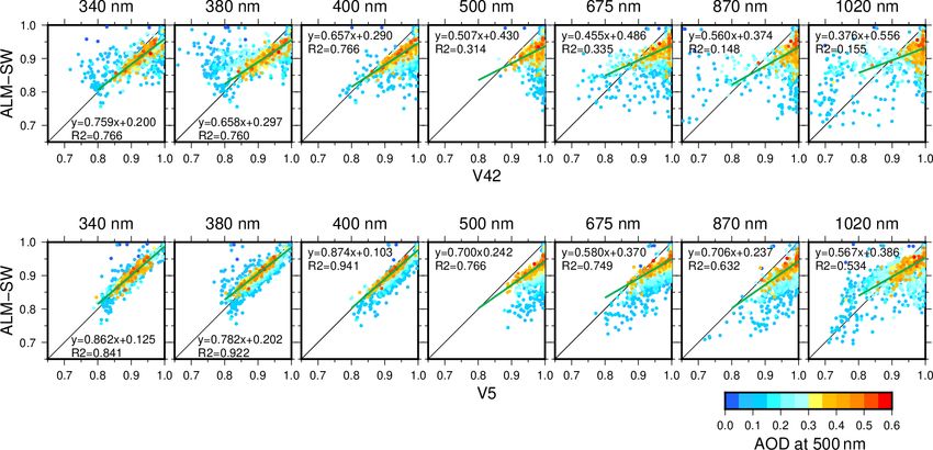
3398                                                          R. Kudo et al.: Optimal use of the Prede POM sky radiometer

diffuse irradiances are measured by the same sensor. Only         haran dust with aircraft in situ measurements performed
diffuse radiance at scattering angles larger than 3◦ is used      and integrated in the vertical. Two flights were success-
in MRI v2, since at the scattering angle of 2◦ abnormally         fully carried out under clear-sky conditions on 16 and 25
large values were seen in the data. In addition, the diffuse      August near Praia (14.948◦ N, 23.483◦ W; 128 m a.s.l.) and
radiances at 1627 and 2200 nm at scattering angles higher         Sal (16.733◦ N, 22.935◦ W; 60 m a.s.l.) islands at the Cape
than 30◦ were removed because of the weak scattering of so-       Verde archipelago, respectively. Saharan dust originating
lar radiation and low sensitivity of the detector at 1627 and     from Africa was observed during the two flights with AOD
2200 nm (Uchiyama et al., 2019).                                  at 500 nm higher than 0.5 and 0.2, respectively. More details
   The calibration constants at 340, 380, 400, 500, 675, 870,     from the field campaigns were made available by Marenco et
940, 1020, 1627, and 2200 nm were transferred from our ref-       al. (2018) and Ryder et al. (2018).
erence sky radiometer by side-by-side comparison. The ref-           A sky radiometer model POM-01 was deployed at Praia
erence sky radiometer was calibrated by the Langley method        airport during SAVEX-D. We applied Skyrad MRI v2 to the
using observation data at the NOAA Mauna Loa observa-             sky radiometer data for the solar direct irradiances and the
tory in Hawaii, USA (19.54◦ N, 155.58◦ W; 3397.0 m a.s.l.)        diffuse radiances in the ALM geometry at the wavelengths
(Uchiyama et al., 2014b, 2018a). The calibration constant at      of 443, 500, 675, 870, and 1020 nm (Estellés et al., 2018).
315 nm was determined by accounting for the TO3 measured          Note that even measurements at a non-standard wavelength
by the Brewer spectrophotometer at the Aerological Obser-         of 443 nm can be processed by our algorithm, since wave-
vatory, Japan Meteorological Agency, located next to the Me-      lengths used in our retrieval method can be flexibly cus-
teorological Research Institute. The calibration procedure for    tomized to the measurements. In this study, the VSD, RRI,
315 nm is described in Appendix A.                                IRI, SSA, and ASM of the MRI v2 products were compared
   Completely clear-sky conditions are required for accurate      with those derived from the in situ measurements (Ryder et
retrievals. Therefore, in Sect. 5.1, we selected clear-sky con-   al., 2018). The details of the aircraft in situ measurements
ditions based on the method by Kudo et al. (2010). The            and methods to derive the aerosol physical and optical prop-
method judges the clear-sky condition from the temporal           erties were described in Ryder et al. (2018).
variations of the surface solar irradiance measured by a co-
located pyranometer.
   The measurements of the surface solar irradiances at the       3     Algorithms
Aerological Observatory under clear-sky conditions were
used for verifying the simulated surface solar irradiances        3.1     Retrieval of aerosols, precipitable water vapor, and
using the retrieved aerosol properties, PWV, and TO3. The                 total ozone
Aeorological Observatory is a station of BSRN (Baseline
                                                                  3.1.1    Inversion strategy
Surface Radiation Network; Driemel et al., 2018). The so-
lar direct and hemispheric diffuse irradiances are measured       Our retrieval method is based on an optimal estimation tech-
by a pyrheliometer (Kipp & Zonen CHP1) and pyranometer            nique similar to the one employed in the AERONET retrieval
(Kipp & Zonen CMP22) with a shading ball in front of the          (Dubovik and King, 2000). The VSD, RRI, IRI, PWV, and
sun. The global irradiances are obtained by the sum of the        TO3 are simultaneously optimized to all the measurements
direct and hemispheric diffuse irradiance measurements. The       of the sky radiometer and all the a priori constraints. The best
pyrheliometer and pyranometer are regularly calibrated once       solution is obtained by minimizing the objective function,
every 5 years by the Japan Meteorological Agency and trace-
able to the WRR (World Radiometric Reference). The pyrhe-                             T  −1
liometer and pyranometer used in this study were calibrated       f (x) = y obs − y(x)     W2     y obs − y(x)
in January 2017 and July 2016, respectively. The BSRN mea-                         −1
surement errors are 2 % for global, 0.5 % for direct, and 2 %           + y a (x)T W2a   y a (x),                             (4)
for diffuse irradiance (McArthur, 2005).
                                                                  where x is a state vector to be optimized, the vector y obs rep-
2.2    SAVEX-D                                                    resents measurements, the vector y(x) represents the simula-
                                                                  tions by the forward model corresponding to y obs , W2 is the
The Sunphotometer Airborne Validation Experiment in Dust          covariance matrix of y, the vector y a (x) is an a priori con-
(SAVEX-D) was conducted in August 2015 at the Cape                straint for x, and Wa is an associated covariance matrix. The
Verde archipelago (Estellés et al., 2018) in conjunction          minimization of f (x) is conducted with the algorithm de-
with two airborne campaigns: AERosol properties – Dust            veloped by Kudo et al. (2016). A logarithmic transformation
(AER-D) and Ice in Clouds Experiment – Dust (ICE-                 is applied to x and y. The minimum of f (x) in the log(x)-
D) over the eastern tropical Atlantic. The main objec-            space is searched by the iteration of x i+1 = x i + αd, where
tive of SAVEX-D was the validation of the SKYNET and              vector d is determined by the Gauss–Newton method, and
AERONET aerosol products in conditions dominated by Sa-           a scalar α is determined by the line search with the Armijo

Atmos. Meas. Tech., 14, 3395–3426, 2021                                              https://doi.org/10.5194/amt-14-3395-2021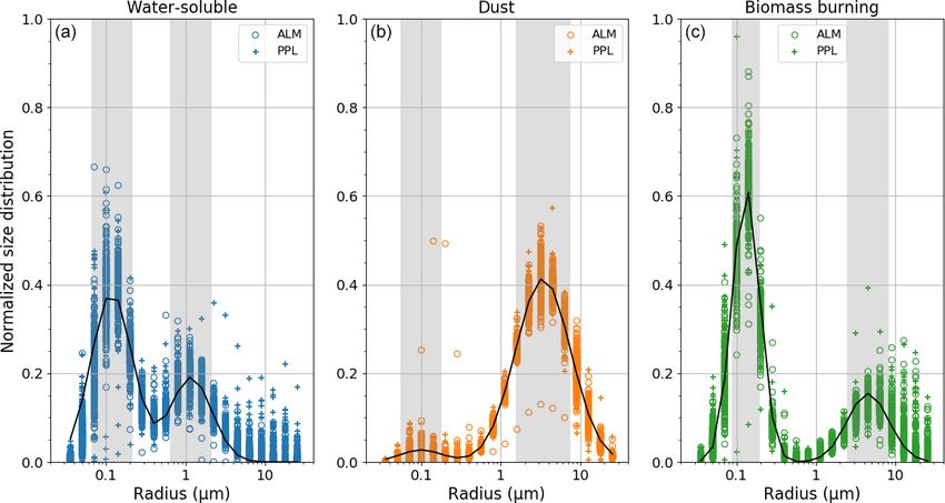
R. Kudo et al.: Optimal use of the Prede POM sky radiometer 3399
rule. The details of the measurements (y obs ) and state vector 2200 nm, as well as the parameters describing VSD. We as-
(x) are described in Sect. 3.1.2. The forward model (y(x)) sumed that the VSD consists of spherical and non-spherical
is introduced in Sect. 3.1.3. The a priori constraint (y a (x)) particles and is expressed as the combination of 20 lognor-
is described in Sect. 3.1.4. Skyrad v4.2–v5 and MRI v1 also mal distributions in the range of the particle radius from 0.03
employ the optimal estimation technique using a similar cost to 30.0 µm:
function as in Eq. (4), but a priori constraints are different.
20
This is also described in Sect. 3.1.4. The Gauss–Newton dV (r) X 1 ln r − ln rm,i
method used for the minimization of Eq. (4) is an iterative = Ci exp − (6)
d ln r i=1
2 si
method and requires an initial value of x. We describe the
20 n
initial value and final outputs in Sect. 3.1.5. X 1 ln r − ln rm,i
= εi Ci exp − ,
i=1
2 si
3.1.2 Measurement and state vectors o
1 ln r − ln rm,i
+ (1 − εi ) Ci exp − , (7)
The y obs comprises transmittances at the wavelengths of 315, 2 si
340, 380, 400, 500, 675, 870, 940, 1020, 1627, and 2200 nm
1, ri < rlm
and the normalized diffuse radiances at scattering angles εi = , (8)
ε, ri ≥ rlm
larger than 3◦ in the ALM or PPL geometries. Note that the
wavelengths and scattering angles used in our method can be where r is the particle radius, V (r) is volume, and Ci , rm,i ,
arbitrarily selected. For example, we used the wavelengths of si , and εi are the maximum volume, center radius, width, and
443, 500, 675, 870, and 1020 nm in Sect. 5.2. volume ratio of the spherical particle to the sum of spherical
Similarly to the retrieval methods of Dubovik and King and non-spherical particles for each lognormal distribution,
(2000) and Kobayashi et al. (2010), the covariance matrix respectively. The first term of Eq. (7) refers to spherical par-
W2 of Eq. (4) was assumed to be diagonal, and the values ticles and the second term to non-spherical particles. rlm is
were given by the measurement errors of the transmittance a radius to separate dV (r)
d ln r into the fine and coarse modes. It
and normalized diffuse radiance. The measurement error of is defined as the radius at the local minimum of the dV (r)
the transmittance mainly depends on the uncertainty of the d ln r
and is determined at every iterative step of x i+1 = x i + αd
calibration constant. Uchiyama et al. (2018a) estimate the in the minimization process of f (x). We assumed that the
error of the calibration constant determined by the Langley fine mode comprises only spherical particles, and the coarse
method using observation data at the NOAA Mauna Loa Ob- mode is a mixture of non-spherical and spherical particles
servatory to be from 0.2 % to 1.3 %, and the error due to with a ratio of ε. The optimized parameters of the size distri-
the transfer of the calibration constant from the reference in- bution are Ci and ε. rm,i is fixed by the radius that separates
strument by the side-by-side comparison was from 0.1 % to the range of 0.03 and 30 µm at log-spaced intervals, ln 1r.
0.5 %. Therefore, we assumed the value of 2 % as the mea- The si is also fixed by ln 1r/1.65 ' 0.21. The value of 1.65
surement error of the transmittances at all the wavelengths. is empirically selected from the range of si that satisfies the
The measurement errors of normalized diffuse radiances are following two conditions. The first condition determines the
defined as 5 % in the work of Kobayashi et al. (2006). We maximum value of si . The observed width of the fine mode
also employed the same value, but we introduced a dynamic of the VSD is smaller than that of the coarse mode and is
weight factor depending on the AOD as follows: about 0.4 (Dubovik et al., 2002). Since we express the VSD
( " # )
0.3 2 as the combination of the lognormal distributions (Eq. 6), the
W = min 5 % · max , 1.0 , 100 % , (5) si should be smaller than 0.4. The second condition is the
τA (λ)
minimum value of si . The dV (r)
d ln r at the middle
radius of two
where τA (λ) is the AOD at wavelength λ. This factor in- lognormal distributions, ln(r) = 0.5 ln rm,i + ln rm,i+1 ,
creases with a decrease in AOD and takes into account the should be larger than 0.5 (Ci + Ci+1 ). If not, the shape of
dV (r)
fact that the absolute value of the diffuse radiance, as well d ln r has unnatural oscillations. Hence, the si should be
as the signal-to-noise ratio, decreases with decreasing AOD. larger than ln 1r/2.35, where 2.35si is the full width at half-
In actual measurements, the angular distribution of the dif- maximum of the lognormal distribution.
fuse radiances at 1627 and 2200 nm has unnatural oscilla- The admitted radii of the VSD range from 0.03 to 30 µm in
tions with scattering angles in the cases of low AOD. This MRI v2. However, the radius range of the previous SKYNET
is due to the low signal-to-noise ratio of the detector at 1627 retrieval methods is from 0.01 to 20.0 µm. The radius range
and 2200 nm (Uchiyama et al., 2019). When τA (λ) is more used in the AERONET retrieval is from 0.05 to 15 µm. We
than 0.3, the value of W is 5 %. The value of 0.3 was empir- investigated the radius range that can actually be estimated
ically determined through many trials by applying different from all the sky radiometer data by a similar technique as in
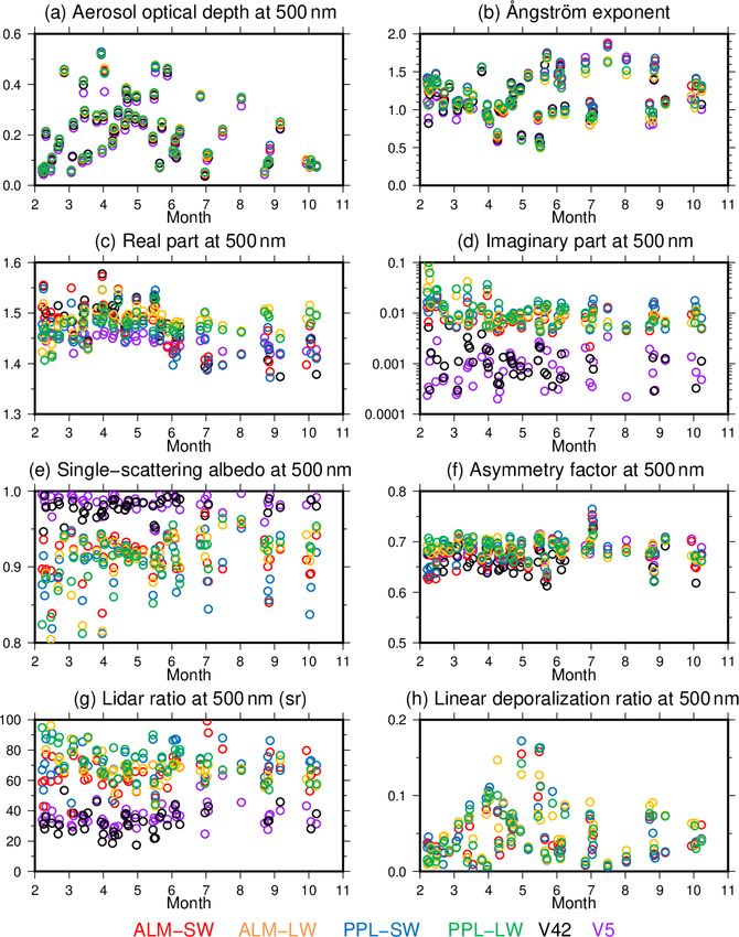
values of τA (λ) to the measurements at Tsukuba. Tonna et al. (1995). Figure A2 shows the Mie kernel func-
The components of x are the PWV, TO3, RRI, and IRI tions of scattering and extinction for wavelengths from 315
at 315, 340, 380, 400, 500, 675, 870, 940, 1020, 1627, and to 2200 nm and scattering angles from 2 to 120◦ . We can see
https://doi.org/10.5194/amt-14-3395-2021 Atmos. Meas. Tech., 14, 3395–3426, 2021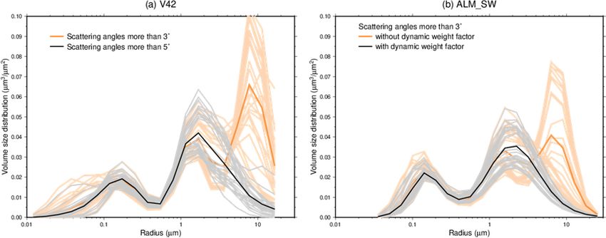
3400                                                           R. Kudo et al.: Optimal use of the Prede POM sky radiometer

that sky radiometer measurements carry information on the          sun. For only the calculation at wavelengths of 315, 940,
VSD in the radius range from approximately 0.02 to 30 µm.          and 2200 nm, the response function of the interference fil-
When we limit the scattering angle range from 3 to 60◦ and         ter of the sky radiometer was taken into account because
the wavelength range from 340 to 1020 nm, the radius range         the spectral changes in the absorption of ozone and water
that can be retrieved is roughly from 0.03 to 10 µm. We might      vapor within the filter bandwidth cannot be ignored. We di-
retrieve giant particles around 20 µm from diffuse radiances       vided the 315 and 940 nm bands into five sub-bands and the
at the wavelengths of 1627 and 2200 nm at a scattering angle       2200 nm band into three sub-bands. For other wavelengths,
of 2◦ . In practice, the measurement errors of the diffuse radi-   the monochromatic calculation was assumed. We also incor-
ances at the scattering angle of 2◦ are too large for almost all   porated the vector radiative transfer model, PSTAR (Ota et
wavelengths. However, we extended the retrieval range of the       al., 2010), as an alternative to the scalar model RSTAR. The
size distribution to the radius of 30 µm for the following rea-    two radiative transfer codes can be easily switched. The op-
son. The size distribution up to 20 µm can be retrieved using      tion of the PSTAR will be useful if polarization measure-
measurements at 1627 and 2200 nm at the scattering angle of        ments, such as in AERONET (Holben et al., 1998), are intro-
3◦ . Since we constrain the size distribution at both ends of      duced to the sky radiometer in the future. Furthermore, we
the radius range to low values by the smoothness constraint        parallelized the codes of RSTAR and PSTAR using OpenMP
of Eq. (10), the size distribution at radii larger than 20 µm is   because radiative transfer calculations at the wavelengths
necessary. In addition, we might be able to use the measure-       from 315 to 2200 nm are time-consuming.
ments at a scattering angle of 2◦ in the future.
                                                                   3.1.4   A priori constraints
3.1.3   Forward modeling
                                                                   A smoothness constraint for the refractive index and size
The forward model y(x) calculates the transmittances and           distribution is necessary for a stable retrieval (Dubovik and
the normalized diffuse radiances from x. The aerosol extinc-       King, 2000). We constrained the spectral dependencies of
tion and scattering coefficients, as well as the phase func-       the RRI and IRI by limiting the values of the following first
tion for the spherical particles, are calculated by the Mie the-   derivatives of the refractive index with the wavelength
ory. For the non-spherical particles, we employed the optical                   ln(n(λ )) − ln(n(λ ))
                                                                                           i            i+1
properties of the randomly oriented spheroids with a fixed         y a (x) = · · ·
                                                                                        ln(λi ) − ln(λi+1 )
aspect ratio distribution, which is optimized to the laboratory               ln(k(λi )) − ln(k(λi+1 ))
measurement of mineral dust (feldspar sample) phase matri-                ···                           ··· ,
                                                                                 ln(λi ) − ln(λi+1 )
ces (Dubovik et al., 2006). The vertical profile of aerosols
can be customized, but at this first stage it is assumed to be            (i = 1, · · ·Nλ − 1),                               (9)
constant from the surface to the altitude of 2 km.                 where n and k are the RRI and IRI at the wavelength λ, and
   The gaseous absorption coefficients for water vapor and         Nλ is the number of wavelengths. For the VSD, the second
ozone are calculated by the correlated k-distribution (CKD)        derivatives of Ci (Eq. 6) with respect to the particle radius
method according to the inputs of the PWV and TO3. The             are introduced by
data table for the CKD method is developed by Sekiguchi
and Nakajima (2008) using the HITRAN 2004 database. The            y a (x) = (· · · ln (Ci−1 ) − 2 ln(Ci ) + ln(Ci+1 )· · ·)
vertical profile of ozone is given from the 1976 version of                                                        0
                                                                   (i = 1, · · ·20), C0 = 0.1 × C10 , C21 = 0.1 × C20 ,        (10)
the US standard atmosphere. The vertical profiles of water
vapor, temperature, and pressure are also given from the US        where C0 and C21 are the volumes outside the radius range
1976 standard atmosphere, but we can optionally select other       from 0.03 to 30.0 µm, and C10 and C20 0 are the initial values of

auxiliary data. For example, the daily measurements of the         Ci in the iteration of the Gauss–Newton method (Sect. 3.1.5).
radiosonde launched at 00:00 UTC at the Aerological Obser-         The small values of C0 and C21 prevent C1 and C20 from be-
vatory were used in Sect. 5.1, while the US 1976 standard          ing abnormal values. The denominator of the second deriva-
atmosphere was used in Sect. 5.2. Other than water vapor           tive was ignored because the rm,i has an equal interval.
and ozone, the gaseous absorption of CO2 , N2 O, CO, CH4 ,            Skyrad v4.2–v5 and MRI v1 use a similar cost function as
and O2 is considered in the forward model. Their vertical          in Eq. (4), but a priori constraints are different. Skyrad v4.2
profiles were given from the standard atmosphere, and their        and MRI v1 employ similar smoothness constraints for the
absorption coefficients were calculated by the CKD method.         RRI, IRI, and VSD, but Skyrad v5 does not use them. MRI
   The solar direct irradiances and the diffuse radiances in       v1 and Skyrad v5 employ a priori estimates for the RRI, IRI,
the ALM and PPL geometries are calculated by the radia-            and VSD. This restricts the range of the solution but is useful
tive transfer model, RSTAR (Nakajima and Tanaka, 1986,             to eliminate unrealistic values. MRI v2 does not use a pri-
1988). The diffuse radiances were calculated using the IMS         ori estimates, similarly to the AERONET algorithm, which
method (Nakajima and Tanaka, 1988), which is an approx-            successfully retrieves the RRI, IRI, and VSD without a priori
imation method to simulate the diffuse radiances near the          estimates (Dubovik and King, 2000).

Atmos. Meas. Tech., 14, 3395–3426, 2021                                               https://doi.org/10.5194/amt-14-3395-2021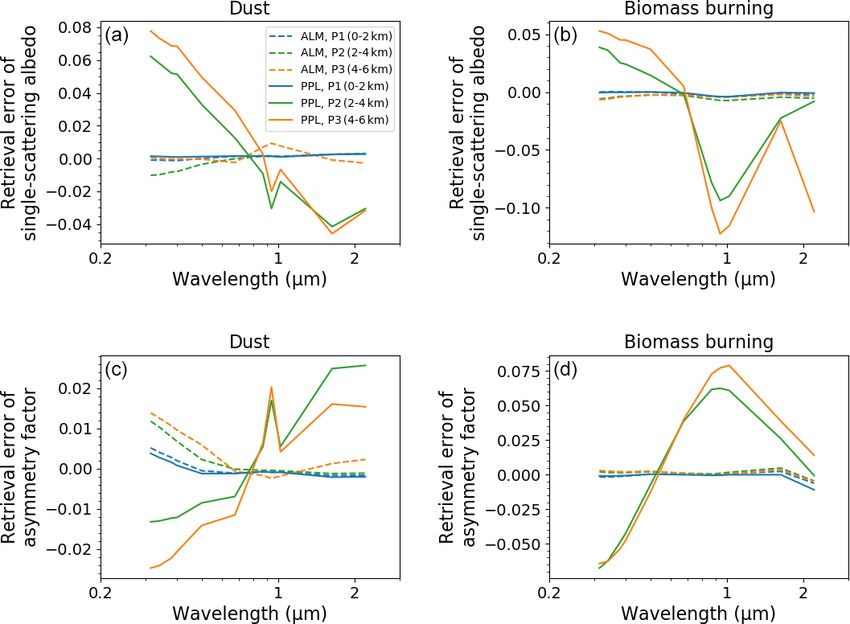
R. Kudo et al.: Optimal use of the Prede POM sky radiometer                                                                   3401

   The covariance matrix W2a in Eq. (4) determines the                After finding the best solution of x, the VSD, RRI, IRI,
strength of the smoothness constraints. We assumed that the        AOD, SSA, ASM, and phase function are provided as out-
matrix is diagonal, and the values of each element corre-          put. In addition, we calculate the LIR and DEP because these
sponding to the RRI, IRI, and VSD are set empirically. The         are important optical properties in synergistic analyses using
typical ranges of the RRI and IRI for tropospheric aerosols        both the sky radiometer and lidar observations.
are from 1.4 to 1.6 and from 0.005 to 0.05, respectively, at the      The objective function of Eq. (4) is a measure of how much
visible and near-infrared wavelengths (Dubovik and King,           the x is optimized to the y obs . However, the objective func-
2000). We therefore defined the values of W2a as                   tion includes the terms of the a priori constraints and does
                                                                   not imply a fitting to only y obs . Therefore, we output another
      ln (1.6) − ln(1.4) ∼                                         measure of the fitness,
Wa =                     = 0.07 for RRI,                   (11)
     ln(2200) − ln(315)
     ln (0.05) − ln(0.005) ∼
                                                                              v
                                                                              u y obs − y(x)T W2 −1 y obs − y(x)
                                                                              u
Wa =                       = 1.2 for IRI.                  (12)
      ln(2200) − ln(315)                                           fobs (x) =
                                                                              t
                                                                                                                    ,          (14)
                                                                                               Ny
   The typical VSD is expressed by a bimodal lognormal
distribution. The AERONET retrievals obtained in different
aerosol conditions around the world (Dubovik et al., 2002)         where Ny is the number of elements in the vector y obs . Equa-
show that the width of the lognormal distribution for the fine     tion (14) is the mean of the differences between the sky ra-
mode is about half of that for the coarse mode. This suggests      diometer measurements and ones calculated from the x by
that the second derivative of the fine mode with respect to        the forward model, weighted by their respective experimen-
the particle radius is also larger than that of the coarse mode.   tal uncertainties. We can filter out the retrievals that are not
Therefore, different values of Wa were given to the fine and       well optimized to the measurements by giving a threshold to
coarse modes:                                                      fobs (x). We used the threshold of 1.0, and the retrieval results
                                                                  that did not satisfy the condition of fobs (x) > 1.0 were dis-
          1.6, ri < rlm                                            carded in this study. This means that almost all the elements
Wa =                       .                                (13)
          0.6, ri ≥ rlm                                            of the vector y(x) lie in the range of y obs ± W.

These values were empirically determined based on the work         3.2   Surface solar irradiance
of Dubovik and King (2000) and through numerous trial-
and-error processes using the measurements of the SAVEX-           In the study of aerosol–radiation interaction, it is important
D campaign.                                                        to ensure consistency between the observed and simulated
                                                                   surface solar irradiances. For this radiative closure study, the
3.1.5   Initial values and outputs                                 global, direct, and diffuse components of the surface solar
                                                                   irradiance in the wavelength region from 300 to 3000 nm
The objective function (Eq. 4) is minimized by the iteration
                                                                   were calculated from the retrieved aerosol optical properties,
of the Gauss–Newton method. The iterative method requires
                                                                   PWV, and TO3, and we compared them with those observed
the initial value of x. The initial values of the RRI and IRI
                                                                   at the Aerological Observatory in Sect. 5.1.
are given as 1.50–0.005i at all the wavelengths. The ratio
                                                                      The surface solar irradiances were calculated by our de-
of the spherical particles in the coarse mode, ε, is 0.1. The
                                                                   veloped radiative transfer model (Asano and Shiobara, 1989;
volume of each lognormal distribution, Ci , is given from the
                                                                   Nishizawa et al., 2004; Kudo et al., 2011). Note that this
size distribution created by the following procedure.
                                                                   model is different from RSTAR and PSTAR used in the for-
 1. AOD at weak gas absorption wavelengths of 340, 380,            ward model of MRI v2. The solar spectrum between 300 and
    400, 500, 675, 870, and 1020 nm is directly calculated         3000 nm was divided into 54 intervals. Gaseous absorption
    from the direct irradiances.                                   by water vapor, carbon dioxide, oxygen, and ozone was cal-
                                                                   culated by the CKD method. The inputs to the radiative trans-
 2. Consider a bimodal size distribution with fixed mode           fer model are AOD, SSA, and phase function at 54 wave-
    radii of 0.1 and 1.0 µm and widths of 0.4 and 0.8 for the      lengths from 300 to 3000 nm. These were calculated from
    fine and coarse modes, respectively.                           the retrieved VSD, RRI, and IRI. The RRI and IRI at wave-
                                                                   lengths between 315 and 2200 nm were interpolated from the
 3. The volume ratio between the fine and coarse modes is          retrieved RRI and IRI in the log–log space. For wavelengths
    fitted to an Ångström exponent obtained from the AOD           less than 315 nm and more than 2200 nm, the retrieved RRI
    in step (1).                                                   and IRI at 315 and 2200 nm were used. A main advantage
                                                                   of MRI v2 is that the aerosol optical properties are retrieved
 4. The total volume of the size distribution is fitted to the     in a wavelength range covering almost the whole shortwave
    AOD at 500 nm.                                                 band.

https://doi.org/10.5194/amt-14-3395-2021                                             Atmos. Meas. Tech., 14, 3395–3426, 2021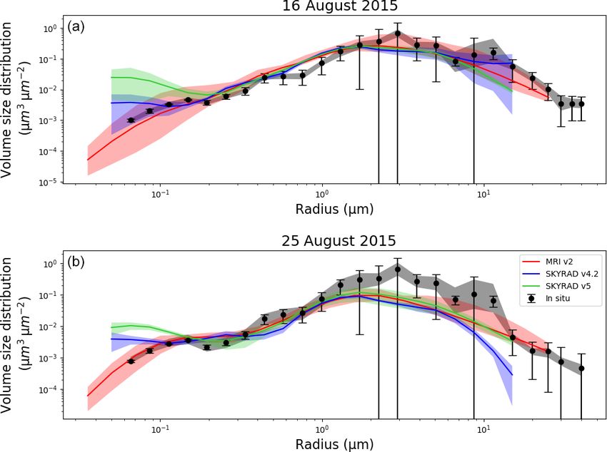
3402 R. Kudo et al.: Optimal use of the Prede POM sky radiometer
4 Uncertainties in retrieval products lengths were biased in the results of the IRI, SSA, and LIR of
the water-soluble and biomass burning models (bias +179 %
4.1 Radiometric uncertainties and +59 %, respectively, with an uncertainty of ±400 % to
450 %). This is because the AOD of the two aerosol mod-
The uncertainties of the MRI v2 retrieval products were eval- els is low at near-infrared wavelengths. Conversely, the re-
uated using the simulations of the sky radiometer measure- trieval errors at the near-infrared wavelengths for the dust
ments. The simulation was conducted for the three aerosol model were smaller (bias +3 %, uncertainty 30 %). The re-
models of water-soluble, dust, and biomass burning (Ta- trieval errors of the DEP for the biomass burning also were
ble 1) used in the accuracy assessment of the AERONET more than 100 %. The reason for the large retrieval error is
retrieval (Dubovik et al., 2000). In the simulation, normally that the simulated value of the DEP is near zero.
distributed random errors were added to direct irradiances, Figure 2 illustrates the retrieved VSD for three aerosol
diffuse radiances, and surface albedo. The standard devia- models. The VSD is normalized to the total volume. The
tions used in generating the random errors are described in shaded area shows the radius range around the fine- and
Table 2. The AOD, solar zenith angle, PWV, and TO3 used in coarse-mode peaks (mode radius ± 1 standard deviation).
the simulation were randomly selected from the ranges in Ta- The bias and uncertainty of the VSD in Table 3 are cal-
ble 1. We conducted 200 simulations for each of three aerosol culated from the results in the shaded areas. The biases of
models and two scanning patterns of the ALM and PPL ge- the retrieval errors around the fine- and coarse-mode peaks
ometries. Our retrieval method was applied to a total of 1200 were less than 22 % (Table 3), but the uncertainties were not
simulation datasets. In 98 out of the 1200 results, fobs (x) was small (Fig. 2). The retrieval errors were also large outside
more than the threshold of 1.0. When the perturbations in the the shaded areas (Fig. 2). The retrieval error at a radius larger
simulation data were too large, our retrieval method was not than the coarse-mode radius + 1 standard deviation was more
able to optimize the parameters to the simulation data. The than 100 % for water-soluble and biomass burning models.
98 retrievals were not included in the following results. However, the retrieval error of the dust model was small at
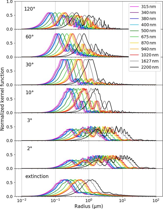
Figure 1 shows the dependencies of the retrieval errors −6 ± 57 % for AOD 0.2 and −9 ± 24 % for AOD > 0.2. The
of SSA on the solar zenith angle and AOD. In this study, VSD at radii up to 30 µm was retrieved well in the dust case.
we define the retrieval error as a deviation of the retrieved In the result of the ALM geometry for the dust model, there is
value from the simulated value for each individual simula- a single subset with a high fine mode and low coarse mode.
tion. When the solar zenith angle is small, the range of scat- Since the AOD at 500 nm used in this simulation was too
tering angle for the diffuse radiance measurements is small, small at 0.26 × 10⁻⁴ , the retrieval failed.
and the available information on the phase function from Overall, the retrieval results at the near-ultraviolet and vis-
the diffuse radiances becomes smaller. We expected that this ible wavelengths were good in the case that the AOD at
would affect the retrieval of aerosols, but no clear depen- 500 nm was larger than 0.2: the absolute values of biases +
dency of the retrieval errors of the SSA on the solar zenith uncertainties in the retrieval products were less than 0.04 for
angle is seen in Fig. 1. The retrieval errors of the other aerosol AOD, less than 0.05 for RRI, less than 130 % for IRI, less
physical and optical properties, PWV, and TO3 also did not than 50 % for VSD, less than 0.05 for SSA, less than 0.02
show any apparent dependencies on the solar zenith angle. for ASM, less than 20 for LIR, and less than 60 % for DEP.
Small AODs make it difficult to retrieve the refractive in- Regardless of the AOD, the retrieval errors of the PWV and
dex because the diffuse radiances are less sensitive to the TO3 were less than 8 mm and 42 m atm-cm, respectively.
refractive index in this case (Dubovik et al., 2000). The re-
trieval errors of the SSA were obviously greater when the 4.2 Uncertainty in the aerosol vertical profile
AOD was smaller than 0.2 (Fig. 1). This dependence on AOD
was also seen in the retrieval errors of the other aerosol phys- In the previous numerical experiments, we investigated the
ical and optical properties. differences of the retrieval errors between the ALM and PPL
The means (bias) and standard deviations (uncertainty) for geometries without finding clear differences. One reason is
the retrieval errors of the aerosol physical and optical proper- that, so far, we have not considered the error from the aerosol
ties, PWV, and TO3 are summarized in Table 3. Note that the vertical profile in the retrieval. The aerosol vertical profile
AOD in Table 3 is calculated from the retrieved VSD, RRI, affects the diffuse radiances in the PPL geometry (Torres et
and IRI and is not directly obtained from the direct solar ir- al., 2014; Momoi et al., 2020). Therefore, we now investigate
radiance. Overall, both the biases and uncertainties of the re- the impacts of the aerosol vertical profile on the retrievals for
trieval errors were large in the case of an AOD less than 0.2. the ALM and PPL geometries. For this purpose, we simu-
In particular, we note a positive bias in the IRI and an uncer- lated the sky radiometer data for the dust and biomass burn-
tainty of more than 100 %. This bias affected the SSA and ing models with different aerosol vertical profiles and con-
LIR, which depend on the IRI. The SSA showed a negative ducted the retrieval with a fixed aerosol vertical profile from
bias and the LIR a positive one. Even if the AOD at 500 nm 0 to 2 km. Three patterns of the aerosol vertical profiles, con-
was more than 0.2, the retrievals at the near-infrared wave- stant from 0 to 2 km (P1), from 2 to 4 km (P2), and from 4 to
Atmos. Meas. Tech., 14, 3395–3426, 2021 https://doi.org/10.5194/amt-14-3395-2021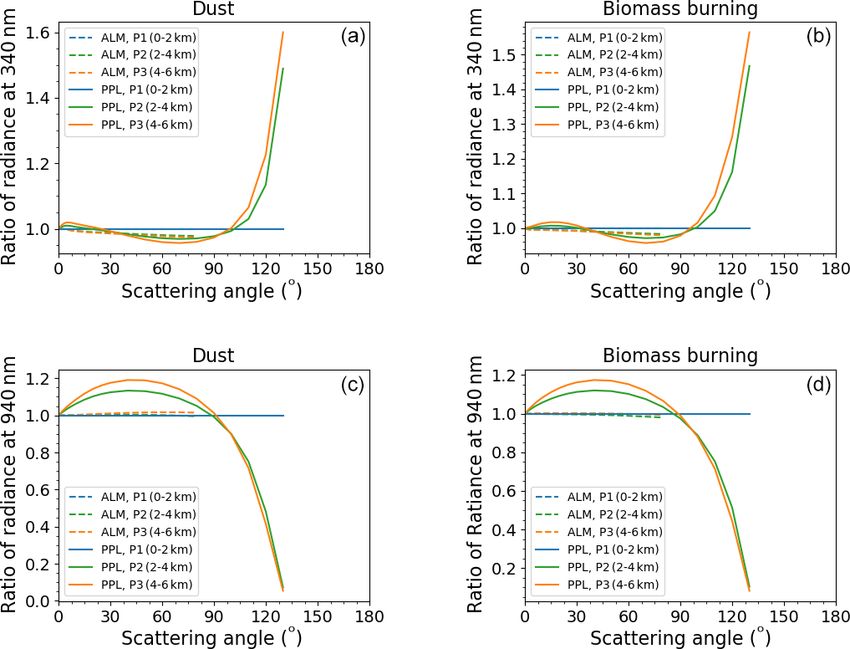
R. Kudo et al.: Optimal use of the Prede POM sky radiometer                                                                             3403

Figure 1. Dependencies of the retrieval errors of the single-scattering albedo at 500 nm on the solar zenith angle (a) and the aerosol optical
depth at 500 nm (b). WS, DS, and BB denote the water-soluble (blue), dust (orange), and biomass burning (green) models, respectively.
ALM and PPL denote the scanning patterns of the almucantar (circle) and principal plane (plus) geometries, respectively.

Figure 2. The retrieved (circle and plus) and simulated (solid line) volume size distributions for water-soluble (left, blue), dust (center,
orange), and biomass burning (right, green). The size distribution is normalized to the total volume. Circle and plus symbols indicate that
the scanning patterns of simulated data are the almucantar (ALM) and principal plane (PPL) geometries, respectively. The shaded area is
the range of the radius around the peak of the fine and coarse modes. The range of the radius around the peak is defined as mode radius ±
1 standard deviation (see Table 1).

https://doi.org/10.5194/amt-14-3395-2021                                                     Atmos. Meas. Tech., 14, 3395–3426, 2021
3404                                                                                 R. Kudo et al.: Optimal use of the Prede POM sky radiometer

Table 1. Configuration of the simulation in the assessment of retrieval uncertainties.

     Aerosol                                                                                         Water-soluble                       Dust           Biomass burning
     Radius (µm)/width of fine and coarse modes                                                0.118/0.6, 1.17/0.6          0.1/0.6, 3.4/0.8           0.132/0.4, 4.5/0.6
     Volume ratio of fine mode to coarse mode                                                                         2                 0.066                               4
     Real and imaginary parts of refractive index at all the wavelengths                              1.45–0.0035i             1.53–0.008i                     1.52–0.01i
     Single-scattering albedo at 340/500/1020 nm                                                    0.97/0.97/0.96          0.83/0.83/0.87                 0.88/0.86/0.73
     Asymmetry factor at 340/500/1020 nm                                                            0.68/0.64/0.63          0.75/0.75/0.75                 0.69/0.60/0.40
     Lidar ratio at 340/500/1020 nm                                                                         62/53/45                78/69/57                      95/75/31
     Linear depolarization ratio at 340/500/1020 nm                                                 0.03/0.05/0.09          0.09/0.15/0.25                 0.00/0.00/0.00
     Aerosol optical depth at 500 nm                                                           Random in the range from 0.0 to 1.0
     Vertical profile                                                                          Constant from 0 to 2 km
     Surface albedo                                                                            0.1 for near-ultraviolet and visible wavelengths, 0.2 for near-
                                                                                               infrared wavelengths
     Solar zenith angle                                                                        Random in the range from 10 to 70◦
     Precipitable water vapor                                                                  Random in the range from 0 to 100 mm
     Total ozone                                                                               Random in the range from 250 to 550 m atm-cm
   The size distribution and refractive index for water-soluble, dust, and biomass burning are cited from Dubovik et al. (2000). Depolarization ratios of the biomass burning
   model are not zero but less than 0.001.

Table 2. Random errors of the simulation in the assessment of retrieval uncertainties.

                           Surface albedo            Normally distributed random deviations with the standard deviation of 0.05
                           Measurement error
                           Direct irradiance         Normally distributed random errors with the standard deviation of 2 %
                           Diffuse radiance          Normally distributed random errors with the standard deviation of 5 %
                         The standard deviations for direct irradiance and diffuse radiances were determined from the works of Uchiyama et al. (2018a)
                         and Kobayashi et al. (2006), respectively.

6 km (P3), were used in the simulation. The constant profile                                 lengths smaller than 870 nm. Only the mean ratios at 940 and
makes it easy to understand the influences of the aerosol layer                              2200 nm, which have strong water vapor absorption, were
altitude. Other parameters were set as follows: the aerosol                                  less than 1.0. The mean ratios at 1020 and 1627 nm were
optical depth at 500 nm was 0.5, the PWV was 30 mm, the                                      about 1.0. The strong diffuse radiances of P2 and P3 at wave-
TO3 was 350 m atm-cm, and the solar zenith angle was 45◦ .                                   lengths smaller than 870 nm for the PPL geometry caused the
   Table 4 summarizes the means for the retrieval errors of                                  underestimation of the IRI (Table 4) and the overestimation
all the parameters, and Fig. 3 shows the retrieval errors of                                 of the SSA (Fig. 3 and Table 4). The weak diffuse radiances
SSA and ASM. The impact of the aerosol vertical profile on                                   of P2 and P3 at 940 and 2200 nm for the PPL geometry in-
the retrieval errors of the aerosol properties, PWV, and TO3                                 creased the IRI and decreased the SSA. The changes in the
for the PPL geometry was larger than that for the ALM ge-                                    diffuse radiances at 1020 and 1627 nm are negligible, but the
ometry. The retrieval errors for the PPL geometry obviously                                  SSA at these wavelengths was underestimated (Fig. 3). This
depend on the aerosol vertical profile. The retrieval errors                                 is because the combined effect of the increased IRI at 940
of SSA for both the dust and biomass burning models were                                     and 2200 nm and the smoothness constraint of the spectral
positive at wavelengths smaller than 870 nm and negative at                                  change for the IRI increased the IRI at 1020 and 1627 nm.
wavelengths larger than 870 nm (Fig. 3). These positive and                                  Consequently, the IRI at all near-infrared wavelengths was
negative errors were related to the diffuse radiances. Figure 4                              overestimated and the SSA was underestimated (Table 4).
shows the mean ratio of the simulated diffuse radiances to                                   Figure 5 plots the ratio of the diffuse radiance to that of P1 at
those of P1 over the scattering angles. The mean ratios of                                   340 and 940 nm. The strong diffuse radiances at wavelengths
P2 and P3 for the PPL geometry were more than 1.0 at wave-                                   smaller than 870 nm for the PPL geometry in Fig. 4 were due

Atmos. Meas. Tech., 14, 3395–3426, 2021                                                                              https://doi.org/10.5194/amt-14-3395-2021
R. Kudo et al.: Optimal use of the Prede POM sky radiometer 3405 Table 3. Means and standard deviations of the retrieval errors. Aerosol model Water-soluble Dust Biomass burning AOD at 500 nm ≤ 0.2 > 0.2 ≤ 0.2 > 0.2 ≤ 0.2 > 0.2 Aerosol optical depth Near-ultraviolet 0.00 ± 0.02 0.01 ± 0.03 0.00 ± 0.02 0.00 ± 0.01 0.00 ± 0.01 0.00 ± 0.02 Visible 0.01 ± 0.01 0.01 ± 0.02 0.00 ± 0.01 0.00 ± 0.01 0.00 ± 0.01 0.00 ± 0.01 Near-infrared 0.00 ± 0.00 0.01 ± 0.02 0.00 ± 0.00 0.00 ± 0.01 0.01 ± 0.02 0.01 ± 0.02 Real part of refractive index Near-ultraviolet 0.04 ± 0.07 0.01 ± 0.04 0.00 ± 0.04 0.00 ± 0.05 0.00 ± 0.07 −0.01 ± 0.04 Visible 0.04 ± 0.06 0.01 ± 0.04 0.00 ± 0.04 −0.01 ± 0.04 0.00 ± 0.07 −0.01 ± 0.03 Near-infrared 0.03 ± 0.05 0.01 ± 0.03 −0.01 ± 0.04 −0.01 ± 0.03 0.00 ± 0.06 −0.01 ± 0.04 Imaginary part of refractive index (%) Near-ultraviolet 800 ± 2460 26 ± 62 25 ± 155 0 ± 24 77 ± 309 −3 ± 21 Visible 827 ± 2475 46 ± 80 24 ± 152 1 ± 25 102 ± 317 3 ± 37 Near-infrared 934 ± 2495 179 ± 410 21 ± 146 3 ± 30 255 ± 450 59 ± 216 Volume size distribution in the radius range around the fine- and coarse-mode peaks (%) Fine mode 4 ± 83 0 ± 27 22 ± 447 6 ± 42 9 ± 40 4 ± 20 Coarse mode 2 ± 21 2 ± 14 2 ± 11 3±9 −5 ± 18 2 ± 13 Single-scattering albedo Near-ultraviolet −0.07 ± 0.13 −0.01 ± 0.02 0.00 ± 0.07 0.00 ± 0.02 −0.03 ± 0.11 0.00 ± 0.02 Visible −0.08 ± 0.14 −0.01 ± 0.02 0.00 ± 0.07 0.00 ± 0.02 −0.06 ± 0.13 −0.01 ± 0.04 Near-infrared −0.12 ± 0.18 −0.05 ± 0.08 0.00 ± 0.06 0.00 ± 0.02 −0.13 ± 0.20 −0.05 ± 0.11 Asymmetry factor Near-ultraviolet 0.01 ± 0.03 0.00 ± 0.01 0.02 ± 0.04 0.01 ± 0.01 0.00 ± 0.02 0.00 ± 0.01 Visible 0.00 ± 0.04 0.00 ± 0.01 0.01 ± 0.03 0.00 ± 0.01 −0.01 ± 0.03 0.00 ± 0.01 Near-infrared −0.01 ± 0.04 0.00 ± 0.01 0.00 ± 0.03 0.00 ± 0.01 0.00 ± 0.04 0.00 ± 0.02 Lidar ratio (sr) Near-ultraviolet 24 ± 54 3±8 4 ± 34 4 ± 12 13 ± 51 −1 ± 11 Visible 16 ± 33 1±5 4 ± 32 −2 ± 10 8 ± 28 0±9 Near-infrared 13 ± 33 3 ± 12 0 ± 23 −3 ± 9 24 ± 42 7 ± 24 Linear depolarization ratio (%) Near-ultraviolet −3 ± 86 −4 ± 47 13 ± 50 7 ± 31 374 ± 530 240 ± 473 Visible −10 ± 75 −12 ± 42 −4 ± 37 −9 ± 27 154 ± 310 90 ± 221 Near-infrared −26 ± 47 −27 ± 34 −18 ± 26 −20 ± 23 −13 ± 130 −24 ± 43 Precipitable water vapor (mm) −0.8 ± 4.1 −1.5 ± 5.8 −1.7 ± 4.9 −1.0 ± 4.3 −0.9 ± 5.8 −1.1 ± 4.5 Total ozone (m atm-cm) −5.0 ± 19.9 −7.4 ± 34.6 1.1 ± 23.9 0.6 ± 24.3 −2.8 ± 22.2 −0.8 ± 34.7 to the large diffuse radiance at scattering angles more than hand, the ratio of the diffuse radiances at 940 nm was large at 90◦ . This increase in the diffuse radiances at backward an- scattering angles smaller than 90◦ and was small at scattering gles became small at longer wavelengths and was negligible angles larger than 90◦ . This was also seen at 2200 nm. This at 1020 and 2200 nm. The increase in the backward scatter- feature and the smoothness constraint for the RRI caused the ing of P2 and P3 for the PPL geometry affects the balance overestimation of the ASM and underestimation of the RRI of the forward and backward scattering and leads to the de- at the near-infrared wavelengths (Fig. 3 and Table 4). crease in the ASM and the increase in the RRI because, as The above experiment suggests that the influence of the predicted by the Mie theory, the ASM decreases with an in- aerosol vertical profile cannot be ignored in the retrieval us- crease in the RRI (Hansen and Travis, 1974). On the other ing the data for the PPL geometry. In practice, the aerosol https://doi.org/10.5194/amt-14-3395-2021 Atmos. Meas. Tech., 14, 3395–3426, 2021
3406                                                                R. Kudo et al.: Optimal use of the Prede POM sky radiometer

Figure 3. Retrieval error of the single-scattering albedo (a, b) and asymmetry factor (c, d) from the simulation data for the dust (a, c) and
biomass burning models (b, d) with different aerosol vertical profiles of 0 to 2 km (blue), 2 to 4 km (green), and 4 to 6 km (orange). The solid
and dashed lines are the retrieval errors for the simulations data in the almucantar (ALM) and principal plane (PPL) geometries, respectively.
Note that the y-axis ranges for dust and biomass burning differ in the plots.

Figure 4. Mean ratio of the simulated diffuse radiances over the scattering angle with aerosol vertical profiles of 0 to 2 km (blue), 2 to 4 km
(green), and 4 to 6 km (orange) to those with the aerosol vertical profile of 0 to 2 km. The left and right panels are the simulations for the
dust (a) and biomass burning (b) models, respectively. The solid and dashed lines are the simulations for the almucantar (ALM) and principal
plane (PPL), respectively.

Atmos. Meas. Tech., 14, 3395–3426, 2021                                                      https://doi.org/10.5194/amt-14-3395-2021
R. Kudo et al.: Optimal use of the Prede POM sky radiometer                                                                         3407

Table 4. Means of the retrieval errors for the almucantar and principal plane geometries.

    Aerosol model                                          Dust                                         Biomass burning
    Altitude of aerosol layer (km)              0–2            2–4                4–6            0–2              2–4             4–6
    Aerosol optical depth
    Near-ultraviolet                    0.00/0.00      0.00/ − 0.03     0.01/ − 0.04        0.00/0.00     0.00/ − 0.02    0.00/ − 0.02
    Visible                             0.00/0.00      0.00/ − 0.01     0.01/ − 0.01        0.00/0.00     0.00/ − 0.01    0.00/ − 0.01
    Near-infrared                       0.00/0.00         0.00/0.01        0.01/0.01        0.00/0.00        0.00/0.00       0.00/0.01
    Real part of refractive index
    Near-ultraviolet                    0.01/0.02         0.01/0.00    0.00/ − 0.03         0.00/0.00        0.00/0.04       0.00/0.03
    Visible                             0.01/0.01         0.01/0.00    0.00/ − 0.02         0.00/0.00        0.00/0.02       0.00/0.02
    Near-infrared                       0.00/0.00      0.00/ − 0.06   −0.01/ − 0.06         0.00/0.00     0.00/ − 0.03    0.00/ − 0.04
    Imaginary part of refractive index (%)
    Near-ultraviolet                       0/ − 3         10/ − 61           −3/ − 70         −1/ − 1         5/ − 41          5/ − 55
    Visible                               −2/ − 3          3/ − 39            0/ − 53         −1/ − 1         2/ − 21          2/ − 35
    Near-infrared                         −5/ − 5           −5/22              −5/13           1/ − 1            1/18             0/37
    Volume size distribution in the radius range around the fine- and coarse-mode peaks (%)
    Fine mode                             −4/ − 5        −7/ − 15               −9/1          −2/ − 1       −1/ − 39         −1/ − 37
    Coarse mode                               1/1            1/11               2/16              4/7            5/9             4/24
    Single-scattering albedo
    Near-ultraviolet                    0.00/0.00       −0.01/0.06         0.00/0.07        0.00/0.00       0.00/0.03      −0.01/0.05
    Visible                             0.00/0.00         0.00/0.03        0.00/0.05        0.00/0.00       0.00/0.01        0.00/0.03
    Near-infrared                       0.00/0.00      0.00/ − 0.03     0.00/ − 0.02        0.00/0.00   −0.01/ − 0.06     0.00/ − 0.09
    Asymmetry factor
    Near-ultraviolet                    0.00/0.00      0.01/ − 0.01     0.01/ − 0.02        0.00/0.00     0.00/ − 0.06    0.00/ − 0.06
    Visible                             0.00/0.00      0.00/ − 0.01     0.00/ − 0.02        0.00/0.00        0.00/0.00    0.00/ − 0.01
    Near-infrared                       0.00/0.00         0.00/0.02        0.00/0.01        0.00/0.00        0.00/0.04       0.00/0.06
    Lidar ratio (sr)
    Near-ultraviolet                          4/3          8/ − 41            6/ − 43         −2/ − 2         1/ − 43          2/ − 45
    Visible                                0/ − 1          2/ − 37            2/ − 40             0/0         1/ − 17          1/ − 21
    Near-infrared                         −2/ − 2          −3/ − 8           −2/ − 13         −2/ − 3          −1/10            −1/16
    Linear depolarization ratio (%)
    Near-ultraviolet                       21/24         17/ − 67            28/ − 81          98/45         90/139           96/347
    Visible                                   5/6         3/ − 78             5/ − 87         33/ − 2         30/37           36/131
    Near-infrared                         −5/ − 4        −8/ − 80            −8/ − 89       −26/ − 47      −29/ − 22        −25/ − 30
    Precipitable water vapor (mm)     −0.4/ − 0.4         −0.3/2.1             4.7/1.3   −0.5/ − 0.5         −0.4/1.8     −0.5/ − 10.6
    Total ozone (m atm-cm)                   1.2/2.3      4.4/42.2           16.7/45.6   −0.7/ − 1.3         0.5/27.2         0.3/46.1

vertical profile has large variability. The synergistic approach         5     Application to real measurements
with lidar is a reasonable solution for this problem (e.g.,
Kudo et al., 2016).                                                      5.1    Application to the measurements at Tsukuba

                                                                         The sky radiometer data collected from February to October
                                                                         2018 in Tsukuba were processed by MRI v2 and Skyrad v4.2
                                                                         and v5 using the following five configurations.
                                                                             1. ALM-SW. Aerosol physical and optical properties were
                                                                                retrieved from the measurements in the ALM geometry.

https://doi.org/10.5194/amt-14-3395-2021                                                     Atmos. Meas. Tech., 14, 3395–3426, 2021
You can also read