A global analysis of the dry-dynamic forcing during cyclone growth and propagation
←
→
Page content transcription
If your browser does not render page correctly, please read the page content below
Weather Clim. Dynam., 2, 991–1009, 2021
https://doi.org/10.5194/wcd-2-991-2021
© Author(s) 2021. This work is distributed under
the Creative Commons Attribution 4.0 License.

A global analysis of the dry-dynamic forcing
during cyclone growth and propagation
Philippe Besson1 , Luise J. Fischer1,2 , Sebastian Schemm1 , and Michael Sprenger1
1 Institute   for Atmospheric and Climate Science, ETH Zürich, Zurich, Switzerland
2 Institute   for Environmental Decisions, ETH Zürich, Zurich, Switzerland

Correspondence: Philippe Besson (phil.besson@bluewin.ch) and Michael Sprenger (michael.sprenger@env.ethz.ch)

Received: 24 March 2021 – Discussion started: 29 March 2021
Revised: 22 September 2021 – Accepted: 29 September 2021 – Published: 27 October 2021

Abstract. Mechanisms driving the intensification and prop-        ing typically occurs earlier, during the growth phase at gene-
agation direction of extratropical cyclones are an active field   sis, while large QGω forcing attains its maximum amplitude
of research. Dry-dynamic forcing factors have been estab-         later towards maturity. (iii) Poleward cyclone propagation is
lished as fundamental drivers of the deepening and propa-         strongest over the North Pacific and North Atlantic, and the
gation of extratropical cyclones, but their climatological in-    poleward propagation tendency becomes more pronounced
terplay, geographical distribution, and relatedness to the ob-    as the deepening rate gets larger. Zonal, or even equatorward,
served cyclone deepening and propagation direction remain         propagation on the other hand is characteristic for cyclones
unknown. This study considers two key dry-dynamic forc-           developing in the lee of mountain ranges, e.g. to the lee of
ing factors, the Eady growth rate (EGR) and the upper-level       the Rocky Mountains. The exact location of maximum QGω
induced quasi-geostrophic lifting (QGω), and relates them         forcing relative to the surface cyclone centre is found to be a
to the surface deepening rates and the propagation direction      good indicator for the direction of propagation, while no in-
during the cyclones’ growth phase. To this aim, a feature-        formation on the propagation direction can be inferred from
based cyclone tracking is used, and the forcing environment       the EGR. Ultimately, the strength of the poleward propaga-
is climatologically analysed based on ERA-Interim data. The       tion and of the deepening is inherently connected to the two
interplay is visualized by means of a forcing histogram,          dry-dynamic forcing factors, which allow cyclone develop-
which allows one to identify different combinations of EGR        ment in distinct environments to effectively be identified.
and QGω and their combined influence on the cyclone deep-
ening (12 h sea-level pressure change) and propagation direc-
tion. The key results of the study are as follows. (i) The ge-
ographical locations of four different forcing categories, cor-   1   Introduction
responding to cyclone growth in environments characterized
by low QGω and low EGR (Q↓E↓), low QGω but high EGR               Extratropical cyclones tend to grow and propagate in narrow
(Q↓E↑), high QGω and low EGR (Q↑E↓), and high QGω                 latitudinal bands known as the storm tracks (Jones and Sim-
and EGR (Q↑E↑), display distinct hot spots with only mild         monds, 1993; Chang et al., 2002; Hoskins and Hodges, 2002;
overlaps. For instance, cyclone growth in a Q↑E↑ forcing en-      Wernli and Schwierz, 2006), but they also occur frequently
vironment is found in the entrance regions of the North Pa-       outside of the main oceanic storm tracks, for example, in sub-
cific and Atlantic storm tracks. Category Q↓E↑ is typically       tropical (Otkin and Martin, 2004; Evans and Guishard, 2009;
found over continental North America, along the southern          Guishard et al., 2009; Evans and Braun, 2012) and in po-
tip of Greenland, over parts of East Asia, and over the west-     lar environments (Mansfield, 1974; Rasmussen and Turner,
ern North Pacific. In contrast, category Q↑E↓ dominates the       2003; Zahn and von Storch, 2008; Simmonds and Rudeva,
subtropics. (ii) The four categories are associated with dif-     2012). During their life cycle, the deepening of extratrop-
ferent stages of the cyclones’ growth phase: large EGR forc-      ical cyclones is supported by a combination of upper- and
                                                                  lower-level forcing mechanisms, and the relative contribu-

Published by Copernicus Publications on behalf of the European Geosciences Union.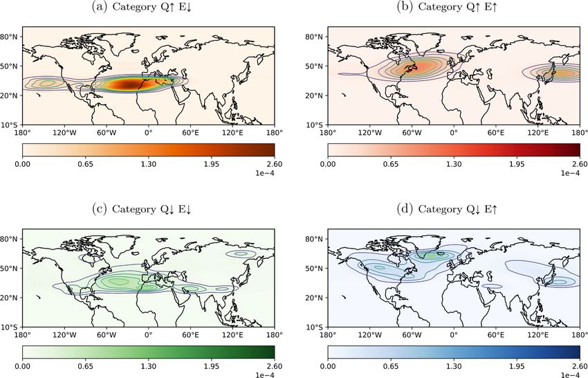
992                                              P. Besson et al.: Cyclone dry-dynamic forcing, deepening and propagation

tions of these forcing mechanisms depend on the cyclone en-       cesses are only indirectly accounted for via their influence
vironment. In general, strong deepening is often driven by        on the low-level baroclinicity. The influence of diabatic pro-
upper-level vorticity advection and flow divergence ahead of      cesses has already been analysed in previous climatologi-
a developing upper-level trough, which results in large-scale     cal studies (Čampa and Wernli, 2012; Boettcher and Wernli,
upward motion (Sutcliffe, 1947; Hoskins et al., 1978; Tren-       2013; Büler and Pfahl, 2017).
berth, 1978; Hoskins and Pedder, 1980; Deveson et al., 2002;          The main motivation for the selection of these two vari-
Gray and Dacre, 2006). At lower levels, it is diabatic heating    ables results from the classical picture of the extratropical
(Rogers and Bosart, 1986; Kuo et al., 1990; Reed et al., 1992;    cyclone development. The classical picture contains two key
Davis, 1992; Whitaker and Davis, 1994; Stoelinga, 1996;           ingredients, which are a low-level zone of enhanced baroclin-
Schemm et al., 2013; Binder et al., 2016) and high baroclinic-    icity, defined as the meridional temperature gradient divided
ity (Charney, 1947; Eady, 1949; Lindzen and Farrell, 1980;        by the static stability, and an upper-level forcing of verti-
Rogers and Bosart, 1986) that accelerate the deepening of         cal lifting that triggers baroclinic growth (e.g. Petterssen and
extratropical cyclones. Consequently, different categories of     Smebye, 1971; Hoskins and Pedder, 1980; Browning, 1990;
cyclones have been established based on different dominant        Semple, 2003). We have chosen to use the Eady growth rate
forcing mechanisms (Petterssen and Smebye, 1971; Deveson          and the QG ω-equation because these two allow for a quan-
et al., 2002; Hart, 2003; Gray and Dacre, 2006; Dacre and         tification of the strength of these two ingredients. The QG
Gray, 2013; Graf et al., 2017; Catto, 2018). In practice, how-    ω quantifies the upper-level forcing of vertical motion, and
ever, the separation between the different forcing mechanism      hence the growth trigger, and the EGR is a measure for the
is often not clear cut, and extratropical cyclones tend to grow   baroclinic growth potential. Note, multiplication of the EGR
within a wide range of these forcing mechanisms.                  with the eddy heat flux would yield a measure for the baro-
   Further, the deepening of extratropical cyclones is inher-     clinic conversion rate (Eq. 4 in Schemm and Rivière, 2019).
ently connected with the direction of propagation. It is long-    We can thus expect strong growth in situations of high EGR
standing knowledge that extratropical cyclones tend to prop-      and QG ω, but we also expect a wide range of possible EGR
agate poleward (Hoskins and Hodges, 2002), but in contrast        and QG ω environments in which cyclone growth occurs.
to tropical cyclones, the mechanisms driving their poleward       Our aim is to quantify this range, relate it to the observed
motion have received enhanced attention only in recent years      cyclone growth rate, and identify regional differences.
(Gilet et al., 2009; Rivière et al., 2012). An upper-level flow       The relevance of this research topic is highlighted by the
anomaly (corresponding to the upper-level trough or positive      fact that the environment and the different forcing factors,
potential vorticity anomaly) that is located to the west of the   which drive extratropical cyclone deepening and the direc-
surface cyclone mutually interacts, by means of an induced        tion of propagation, are expected to change as the climate
circulation, with the positive surface temperature anomaly        warms (Shaw et al., 2016; Catto et al., 2019). Indeed, cli-
(corresponding to a surface anomaly of potential vorticity).      mate projections suggest a decrease in low-level baroclinic-
This interaction enhances the poleward heat flux that in turn     ity due to an amplified warming at higher latitudes, a process
enhances the baroclinic growth (Hoskins et al., 1985; Coro-       known as the Arctic Amplification. On the other hand, the in-
nel et al., 2015; Tamarin and Kaspi, 2016). The combined up-      creased water storage capacity of the atmosphere in a warmer
per and lower-level circulations, which include the so-called     climate suggests a potential increase in the latent heat re-
β-drift, advect the cyclone centre poleward (Gilet et al.,        lease and thus (positive) diabatic impact on cyclone devel-
2009; Rivière et al., 2012; Tamarin and Kaspi, 2016). Rapid       opment. Both changes seem to be engaged in a tug-of-war
deepening and poleward propagation are therefore inherently       (Catto et al., 2019), resulting in a fuzzy picture of how extra-
connected.                                                        tropical cyclones will change in a warmer climate. Changes
   In this climatological analysis, we quantify the regional      in the dry upper-level forcing are not well known. Over-
variability of the upper- and lower-level forcing mechanisms      all, extratropical cyclones are projected to become slightly
during the growth phase, i.e. between genesis and matu-           stronger and less frequent, though the number of extreme
rity, of extratropical cyclones and systematically link this      cyclones likely increases (Lambert and Fyfe, 2006; Ulbrich
information with the direction of propagation. Specifically,      et al., 2008; Bengtsson et al., 2009; Zappa et al., 2013). At
the focus is set on (i) the strength of the upper-level forc-     the same time, the storm tracks are projected to shift pole-
ing, as measured by the quasi-geostrophic (QG) ω-equation         ward (Bengtsson et al., 2009; Chang and Guo, 2012), which
(Hoskins et al., 1978); (ii) the strength of the low-level        could be a result of enhanced poleward propagation (Tamarin
baroclinicity, as measured by the Eady growth rate (EGR)          and Kaspi, 2016).
(Lindzen and Farrell, 1980); and (iii) the link with the cy-          Our study is also an attempt to create a baseline of the
clone deepening rates at the surface and propagation direc-       lower- and upper-level dry-dynamic forcing and its variabil-
tions obtained from a feature-based cyclone track climatol-       ity under present-day climate conditions, which may prove
ogy (Wernli and Schwierz, 2006; Sprenger et al., 2017). In        useful in the assessment of its future changes. The study is
this study, we focus on the mechanisms that reflect the dry-      structured as follows. In Sect. 2, the used datasets (cyclone
dynamic forcing of the cyclone deepening. Diabatic pro-           tracks and forcing factors) are introduced. In Sect. 3, we ad-

Weather Clim. Dynam., 2, 991–1009, 2021                                               https://doi.org/10.5194/wcd-2-991-2021
P. Besson et al.: Cyclone dry-dynamic forcing, deepening and propagation 993
dress the cyclone growth and its link to the forcing factors where Vg denotes the geostrophic wind and φ the geopoten-
and quantify their regional variability. Section 4 considers tial. The forcing from upper levels only is obtained by set-
the direction of cyclone propagation in detail, as it is linked to ting the divergence ∇ · Q to zero for pressure levels from the
cyclone deepening and the forcing factors. Finally, the study surface to 550 hPa. The numerical details of the iterative in-
concludes, in Sect. 5, with a summary, some caveats, and an version of the QG ω-equation follow the description in Stone
outlook. (1968) and Pascal and Sprenger (2009).
The formal definition of EGR is (Lindzen and Farrell,
1980)
2 Data and methods 1/2
f ∂|u| g ∂θ
2.1 ERA-Interim and dry-dynamic forcing EGR = 0.31 with N = ,
N ∂z θ ∂z
The analysis is based on the ERA-Interim dataset from 1979 where |u| is the magnitude of the horizontal wind speed,
to 2016 (Dee et al., 2011), provided by the European Centre θ is potential temperature, and z is height. The discretized
for Medium-Range Weather Forecasts (ECMWF). The mete- form used in this study represents the layer between 850 and
orological fields are available on 60 hybrid-sigma model lev- 500 hPa,
els, have a spatial resolution of 80 km (T255 spectral resolu-
tion), and are temporally structured into 6-hourly time steps. f
EGR = 0.31
We have interpolated the fields onto a global longitude– N500−850
latitude grid with a resolution of 1◦ × 1◦ . The analysis in this " #1/2
u500 − u850 2 v500 − v850 2
study is restricted to the Northern Hemisphere north of 20◦ N × + ,
and covers the extended winter (October–March). z500 − z850 z500 − z850
The ERA-Interim data are used to identify cyclones based
on sea level pressure (SLP). Additionally, secondary fields where uX , vX , and zX are the two horizontal wind compo-
such as Eady growth rate (EGR) and ω forcing (QGω) are nents and the height at the pressure level X, respectively,
calculated according to Graf et al. (2017). We exclusively and N500−850 is a pressure-weighted average of the Brunt–
considered QGω on 500 hPa and restricted it to the forcing Väisälä frequency, which is computed on ERA-Interim
from levels above 550 hPa; i.e. it represents upper-level forc- model levels and later vertically averaged between the two
ing. EGR, on the other hand, is representative for low- to pressure levels. The two variables are not fully independent
mid-tropospheric baroclinicity (850 to 500 hPa). More for- of each other, since the temperature gradient affects the EGR
mally, QGω is calculated by inverting the QG ω-equation, and the Q. The omega forcing is stronger in the presence of
which in the Q-vector formulation reads as follows (Davies, high baroclinicity. Because we analyse low-level EGR, it is
2015): not the same horizontal temperature gradient that intervenes
in the Q vector, which is analysed at upper levels.
∂2
The forcing factors will be determined along all cyclone
2
σ∇ + f02 ω = −2∇ · Q. tracks, i.e. the geographical position of minimum SLP (see
∂p 2
Sect. 2.2 below). It is, however, not reasonable to only con-
Here, f0 denotes the Coriolis parameter and σ the static sta- sider the values of QGω and EGR at the cyclone’s centre,
bility in pressure coordinates, which is defined by which is defined by the location of the minimum SLP, be-
cause the cyclone growth and propagation are determined by
p Tv dθ its larger environment. Hence, we calculated the mean value
σ (p) = − .
R θ dp of EGR and QGω within a 1000 km radius around the cy-
clone centre. For QGω, two mean values were calculated:
The static stability is not constant in the domain. However, one by only considering negative values (corresponding to
to avoid numerical stability problems in situations of near- forcing of upward motion) and a second one considering only
neutral or negative static stability, a 1d vertical profile of positive values (forcing of downward motion). In this way,
the static stability is used in the inversion of the Q-vector we take into account that QGω often appears as a dipole,
equation. The profile is computed as a simple horizontal do- with the effect that the two dipole parts counterbalance each
main average. It has been shown in previous case studies that other if a simple mean is calculated.
this pragmatic choice has only a marginal influence on the fi-
nal outcome of the layer-averaged upper-level forcing (Graf 2.2 Cyclone climatology and time normalization
et al., 2017). The Q vector is defined by
To obtain the cyclone climatology, the identification and
∂Vg
· ∇ ∂φ tracking algorithm by Sprenger et al. (2017) was employed,
∂x ∂p ,
Q = ∂Vg which is a slightly modified version of the algorithm intro-
∂φ
∂y · ∇ ∂p duced by Wernli and Schwierz (2006). First, the algorithm
https://doi.org/10.5194/wcd-2-991-2021 Weather Clim. Dynam., 2, 991–1009, 2021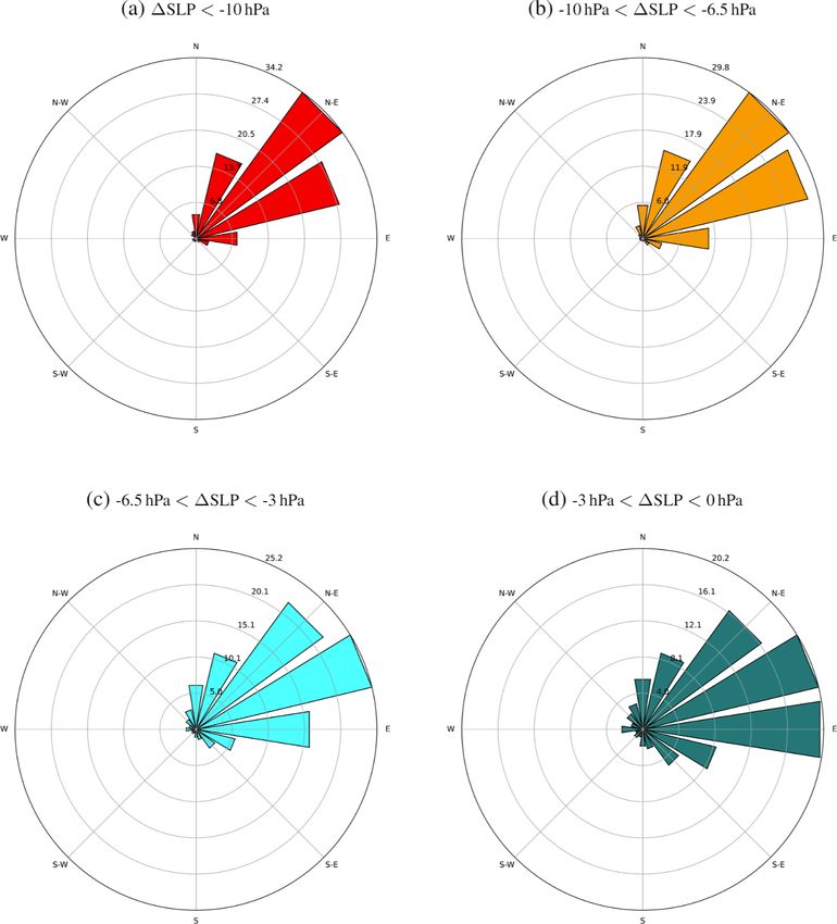
994                                               P. Besson et al.: Cyclone dry-dynamic forcing, deepening and propagation

scans the grid points for SLP minima defined as having a            Hence, in this normalized time frame, tnorm = −1 corre-
lower value than the eight neighbouring SLP values on the           sponds to cyclogenesis, tnorm = 0 to the time instance of min-
grid. Secondly, the cyclone extent is determined by the out-        imum SLP, and tnorm = +1 to cyclolysis. In the remainder of
ermost closed SLP contour encompassing the identified SLP           the study, t always refers to this normalized time. All of the
minima (assuming a 0.5 hPa interval). To exclude spurious,          analysis in Sects. 3 and 4 will be restricted to the phase with
small-scale SLP minima, the enclosing contour has to exceed         normalized times between −1 and 0; i.e. the focus is on the
a minimum length of 100 km, otherwise the SLP minimum               cyclone’s life cycle between genesis and the time instance of
is discarded. In some cases the outermost SLP contour con-          the deepest SLP, i.e. the cyclone growth phase.
tains more than one SLP minimum. If the distance between               Finally, three geographical regions in the Northern Hemi-
two SLP minima within the same outermost enclosing SLP              sphere are particularly considered in this study: North Pacific
contour is less than 1000 km, they are attributed to the same       (25–65◦ N, 125–180◦ E), North Atlantic (25–65◦ N, 75◦ W–
cyclone cluster, creating a multi-centre cyclone. In this case      0◦ ), and North America (25–65◦ N, 120–75◦ W). To be at-
only the lowest SLP minimum is kept, and the others are dis-        tributed to one of these three target regions, a cyclone must
regarded. The central SLP value and its geographical coordi-        be located inside the respective latitude–longitude box at the
nates are stored and subsequently used to determine cyclone         time of genesis.
tracks with cyclogenesis and lysis at the first and final time
steps of the track, respectively. As in Sprenger et al. (2017),
                                                                    2.3   Dry-dynamic forcing categories
the tracks have to exceed a minimum lifetime of 24 h from
genesis to lysis.
   During their life cycle, cyclones can undergo a process          In this study, we frequently employ a 2D histogram, which
called “cyclone splitting”, which occurs when a cyclone (or a       has EGR on the x axis and QGω on the y axis. The histogram
multi-centre system) breaks up and forms two (or more) cy-          consists of 49 linearly distributed bins defined by a range of
clones that then extend from the same origin as two separate        EGR and QGω values such that each bin is characterized by a
cyclone tracks. As a consequence, the newly formed cyclone          specified EGR and QGω forcing. Each 6 h time interval dur-
typically experiences only decay characterized by an increas-       ing a cyclone growth phase is classified according to its EGR
ing SLP over the course of its life cycle. To eliminate this        and QGω values such that each bin is populated by a multi-
subcategory of cyclones from the data, all cyclones that ex-        tude of cyclone time segments from various cyclone tracks.
hibit their minimum SLP value either at genesis or at genesis       The colour shading in each of the bins represents the mean
+6 h are disregarded. In this way, the analysis is restricted to    value over all time steps of a specific cyclone characteris-
cyclones with an archetypal pressure evolution, i.e. starting       tic, for example, the deepening rate. Figure 1 shows such a
with higher pressure at genesis than attained during maturity.      histogram where the mean represents the average per bin of
   Because the lifetime of cyclones can extend from 24 h (by        all 12 h changes in mean sea-level pressure (1SLP). Consid-
the requested minimum duration; see above) to several days          eration is given to all 1SLP changes during the growth pe-
and it is therefore difficult to compare different cyclone life     riod of every life cycle and not only to the maximum change.
cycles, the method of Schemm et al. (2018) is applied to nor-       Therefore, every cyclone contributes with several time steps
malize the cyclone lifetimes. More specifically, three main         to the statistics, and positive 1SLP values are accepted as
time stamps are determined: tgenesis (time of genesis), tmax        long as they occur prior to the time of maximum intensity.
(time of maximum intensity, i.e. minimum SLP), and tlysis           Positive values indicate that the deepening between genesis
(time of lysis). Then 1t1 is computed as the difference be-         and maximum intensity is not linear. If, for instance, a 12 h
tween tgenesis and tmax , which results in a negative value:        1SLP value of 6 hPa is associated with an EGR of 1.2 d−1
                                                                    and a QGω value of −0.01 Pa s−1 , it contributes to the lower
1t1 = tgenesis − tmax .                                             right corner of the histogram. The 12 h 1SLP values in ev-
Next, the difference between tlysis and tmax (indicated as 1t2 )    ery bin will vary between different cyclones, and each bin
is determined, which results in a positive value:                   is therefore populated by a distribution of 12 h 1SLP val-
                                                                    ues. This is illustrated in Fig. 1 for the four corners of the
1t2 = tlysis − tmax .                                               histograms. If not otherwise stated, the colour shading rep-
                                                                    resents the mean values. The distributions of the 12 h 1SLP
For a certain time t between tgenesis and tmax , we can calculate   values resemble Gaussian distributions, but still differ in their
a normalized time tnorm :                                           shapes: some are narrow and centred around 0 hPa, whereas
          tmax − t                                                  others are more broadly distributed. However, none of the
tnorm =            .                                                distributions in Fig. 1 (and also in the results of Sects. 3 and
            1t1
                                                                    4) are strongly skewed with long tails to one end. The num-
The same is done for time t between tmax and tlysis :               ber of cyclone track segments in each bin is of the order of
          t − tmax                                                  several thousands, except for the bins close to the corners of
tnorm =            .                                                the 2D histogram. The specific numbers of cyclone track seg-
            1t2

Weather Clim. Dynam., 2, 991–1009, 2021                                                 https://doi.org/10.5194/wcd-2-991-2021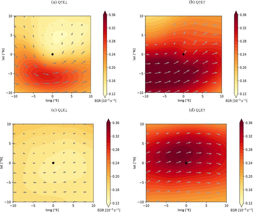
P. Besson et al.: Cyclone dry-dynamic forcing, deepening and propagation 995
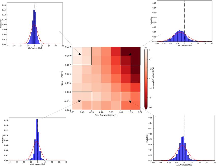
Figure 1. Exemplary 2D forcing histogram with EGR (in d−1 ) on the x axis and QGω (in Pa s−1 ) on the y axis. Colours show the mean
1SLP value for each bin (darker (lighter) red highlights bins containing time intervals with stronger (weaker) mean deepening rates (1SLP)).
For every corner of the histogram (framed in black, consisting of 2 × 2 bins), the distribution of 1SLP values is shown. The four boxes are
used to define four forcing categories: Q↓E↓, Q↓E↑, Q↑E↓, and Q↑E↑ (see text for details).
ments and therefore the number of 1SLP values can be seen 3 Dry-dynamic forcing during cyclone growth
in Fig. S1 in the Supplement.
The lower left corner of the histogram represents low QGω In this section, we study the regional variability of the forc-
and low EGR forcing. Conversely, high QGω and high EGR ing mechanisms during the growth phase of cyclones. We
forcing are located in the upper right corner. The lower right start with the geographical distribution of the four categories
(upper left) corner represents cyclone growth in environ- Q↓E↓, Q↓E↑, Q↑E↓, and Q↑E↑ that were introduced in
ments characterized by low (high) QGω and high (low) EGR Sect. 2.3. Then we proceed in Sect. 3.2 with a detailed anal-
forcing. The four corners of the histogram are used to define ysis of the forcing histogram, and finally, in Sect. 3.3, we
four forcing categories, which are discussed in more detail discuss cyclone-centred composites of QGω and EGR.
in Sect. 3. More specifically, the box in the lower left corner,
for example, is referred to as Q↓E↓ (cyclone growths in a 3.1 Geographical distribution of dry-dynamic forcing
low-QGω Q↓ and low-EGR E↓ environment), and the other
In this section, consideration is given to the geographical
boxes are labelled accordingly.
distribution of the four forcing categories. Density plots are
created by considering all time steps during the cyclones’
growth phase and by computing their inclusiveness to one of
the four forcing categories (Q↓E↓, Q↓E↑, Q↑E↓, or Q↑E↑)
https://doi.org/10.5194/wcd-2-991-2021 Weather Clim. Dynam., 2, 991–1009, 2021
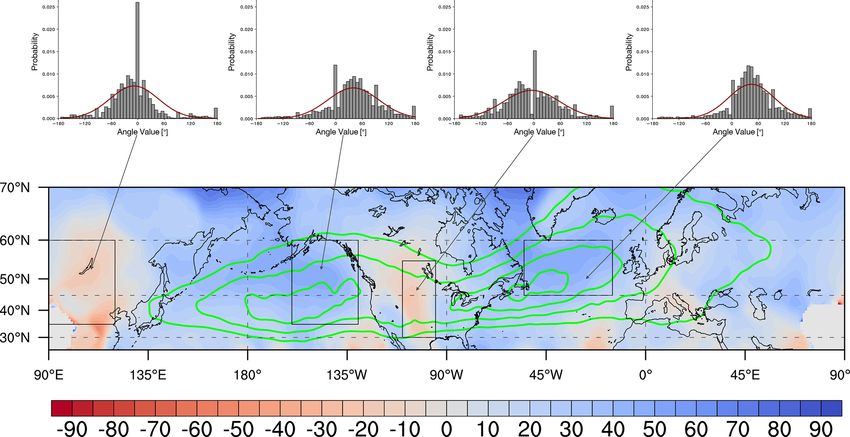
996                                                 P. Besson et al.: Cyclone dry-dynamic forcing, deepening and propagation

Figure 2. Normalized geographical density distribution (coloured contours and filled contours) of the four selected forcing categories: (a)
high QGω forcing and low EGR (Q↑E↓), (b) high QGω and high EGR (Q↑E↑), (c) low QGω and low EGR (Q↓E↓), and (d) low QGω and
high EGR (Q↓E↑). For the exact computation, see text.

and the corresponding latitude–longitude location. The out-             ward of the identified hot spot in Q↓E↑ (Fig. 2d). We hypoth-
come is a remarkably distinct geographical distribution of the          esize that early during the life cycle time steps are catego-
occurrence of the four forcing categories (Fig. 2). The four            rized into Q↓E↑ (Fig. 2d), while afterward during the main
category-specific plots show a probability density distribu-            deepening period both forcings contribute to the deepening,
tion, which integrates to 1. Each forcing category has unique           and the corresponding time steps are categorized into Q↑E↑
hot spots, which are discussed in the following.                        (Fig. 2b). We will come back to this hypothesis in the next
   We start our discussion of the forcing-based categories              section.
(Fig. 1) with category Q↑E↓ (Fig. 2a), which is mostly con-                For category Q↓E↑ (Fig. 2d), the regions where the forc-
fined within a latitudinal band between 25 and 40◦ N. The               ing occurs most frequently are over North America and partly
major hot spot is located over the North Atlantic off the               over the western North Atlantic and further over the southern
west coast of northern Africa and spanning over the Mediter-            tip of Greenland and parts of central Asia. Another promi-
ranean. A second but less dense region is discernible in the            nent hot spot is located over the Pacific Ocean off the coast
Pacific off the US west coast, reminiscent of Kona lows                 of Japan. Over North America, the maximum is located near
(Simpson, 1952; Morrison and Businger, 2001; Moore et al.,              50◦ N and therefore north of the cyclogenesis region down-
2008). The downstream regions are eventually related to sec-            stream of the southern Rocky Mountains in the US (see
ondary or downstream cyclogenesis, though one would ex-                 Fig. 5c in Hoskins and Hodges, 2002). It is connected to cy-
pect high EGR due to the trailing cold fronts typically in-             clone deepening in the lee of the Canadian Rocky Mountains
volved in secondary cyclogenesis (Schemm and Sprenger,                  and the formation of “Alberta clipper” cyclones (Chung and
2015; Schemm et al., 2018; Priestley et al., 2020). Over the            Reinelt, 1973; Thomas and Martin, 2007). The southern tip
Atlantic, this category also comprises the deepening of sub-            of Greenland is a well-known cyclogenesis hot spot (Hoskins
tropical cyclones, which form under strong QGω forcing,                 and Hodges, 2002; Wernli and Schwierz, 2006), and high
provided by equatorward pushing intrusions of high-PV air               baroclinicity in this region is connected to the steep slopes
(Caruso and Businger, 2006) and a weak baroclinic zone.                 of the Greenland shelf. Off the coast of Japan, high baroclin-
   The next category Q↑E↑ (Fig. 2b) has two distinct                    icity is maintained by the Kuroshio sea-surface temperature
hot spots: one northeastward-orientated band reaching from              front, and the density maximum is located slightly equator-
North America to Norway with the maximum frequency                      ward of the maximum of the category Q↑E↑ (Fig. 2b).
northeast of Nova Scotia in the North Atlantic and the other               Finally, for category Q↓E↓ (Fig. 2c) the highest density
hot spot off the coast of Japan. Both are located slightly pole-        is located over the subtropical Atlantic spanning a horizon-

Weather Clim. Dynam., 2, 991–1009, 2021                                                      https://doi.org/10.5194/wcd-2-991-2021
P. Besson et al.: Cyclone dry-dynamic forcing, deepening and propagation                                                        997

tal band from the Gulf of Mexico to North Africa, cover-            the west compared to its negative counterpart. This indicates
ing parts of the Mediterranean Sea and extending down-              that the positive and negative anomalies are most likely part
stream into the Middle East, with a local maximum over              of common weather systems, e.g. to the west and east of a
Iran, and even further downstream over China and into the           short-wave trough.
East China Sea. Over Asia, there is an additional hot spot             In addition to the forcing distribution and climatology of
region upstream of Kamchatka. These two branches over               EGR and QGω, category distributions as in Fig. 2 but for
Asia correspond well with the two seeding branches of the           EGR and QGω separately could be considered. This is pre-
North Pacific storm track described by Chang (2005). The            sented in Fig. S4, whereas these distributions are, for the
cyclones along the southern branch, in contrast to the north-       most part, a combination of the categories shown in Fig. 2.
ern one, are known to be diabatically driven in the early life      For instance, Fig. S4a shows the geographical distribution for
cycle stage (Chang, 2005). The Hudson Bay in Canada is              E↓, which is a combination of Q↑E↓ (Fig. 2a) and Q↓E↓
another localized region where cyclone growth occurs in a           (Fig. 2c). However, for Q↑ (Fig. S4d), the major hot spot
low-QGω- and low-EGR-forcing environment. Surface cy-               over the Atlantic off the coast of northwestern Africa (seen
clone deepening in this region is often connected to the de-        in Fig. 2a) disappears due to a low density relative to other
velopment of a tropopause polar vortex also known as an             regions.
upper-level cut-off low (Gachon et al., 2003; Cavallo and
Hakim, 2009; Portmann et al., 2021). The deepening maxi-            3.2   Temporal evolution of dry-dynamic forcing
mum over the subtropical North Atlantic comprises subtrop-
ical cyclone development (Caruso and Businger, 2006), and           In the previous section, we discussed the geographical dis-
because it is located north of a known Hurricane genesis re-        tribution of the two dry-dynamic forcing mechanisms during
gion, it might also contain some recurving tropical cyclones        the cyclone growth phase. In this section, we discuss their
(Landsea, 1993; McTaggart-Cowan et al., 2008). The smaller          temporal evolution because the dominating forcing mecha-
maximum over western North Africa indicates the deepen-             nism might change during the growth phase. Figure 3a shows
ing of African easterly waves (Burpee, 1972), which often           the forcing histogram, as in Fig. 1, exclusively for the cy-
precede Hurricane formation over the subtropical North At-          clones’ growth phase, and Fig. 3b shows the corresponding
lantic (Landsea, 1993; Avila et al., 2000). It is noteworthy at     normalized life cycle time tnorm (tnorm = −1 corresponds to
this stage that EGR and QGω forcing is low relative to all          genesis and tnorm = 0 to maximum intensity). The strongest
other locations in the Northern Hemisphere where cyclone            deepening is depicted by dark red shading in the upper right
growth occurs; however, the observed EGR and QGω forc-              corner in Fig. 3a. It occurs, not too surprisingly, in a high-
ing might be high relative to a local climatology (see Fig. S2a     QGω and high-EGR environment. The deepening rates in a
and b). Furthermore, it is interesting to relate the density dis-   low-QGω and low-EGR environment (lower left corner in
tribution of the four categories (Fig. 2a–d) into the context       Fig. 3a) are consequently low. However, the upper left and
of the climatological relationship between EGR and QGω.             lower right corners of the forcing histogram differ: the deep-
For example, category Q↑E↑ (Fig. 2b) is found at the begin-         ening rates are larger in a high-EGR and low-QGω environ-
ning of the North Atlantic and Pacific storm tracks. These          ment (lower right) compared to a low-EGR and high-QGω
are regions where the correlation between QGω and EGR               environment (upper left). Potentially this asymmetry is due
(see Fig. S2c) is negative and also somewhat enhanced com-          to the connection between high-EGR environments, for ex-
pared to mid- and east-oceanic regions; i.e. the correlation        ample along a surface front, and diabatic forcing as is the
matches the expectation. However, the link to the other cate-       case for diabatic Rossby wave development (Boettcher and
gories is not particularly strong. With respect to the correla-     Wernli, 2013). However diabatic processes are intentionally
tion between EGR and QGω (Fig. S2c) regardless of the four          disregarded in our analysis. The asymmetry between the two
forcing categories, the correlation remains rather weak in the      opposite corners could also point to a (potentially) subtle dif-
main North Atlantic and Pacific storm tracks, and the corre-        ference in EGR and QGω forcing. It indicates that EGR has a
lation is larger in the western part of the storm tracks, while     stronger influence on the deepening rates than QGω and that
it becomes smaller towards the east. Furthermore, the largest       baroclinic instability might be released as long as there is a
anti-correlations are found in the subtropics east of China and     reasonable (even moderate) amount of upper-level forcing.
west of North America and Africa. Positive correlations are         In short, moderate upper-level forcing (QGω) might be suffi-
essentially restricted to the region east of the Himalayas.         cient to trigger substantial deepening rates if EGR is high. In
   Figure S3 shows the winter climatology for QGω, as in            contrast, if EGR is low, weaker deepening rates result even
Fig. S2b, but for negative (Fig. S3a) and positive (Fig. S3b)       if substantial upper-level forcing is discernible. Furthermore,
QGω values separately. The patterns in both figures are simi-       Fig. S6 shows the forcing histogram with the standard de-
lar, which underlines the fact that the positive and negative       viation of the 1SLP for each bin with colour shading and
anomalies often co-occur in QGω dipoles. Still, there are           the exact value in every bin. The figure indicates that there
noteworthy differences. One specific example is the positive        is not a linear increase in the deepening rates with linearly
pole in the eastern Mediterranean, which is located further to      increasing EGR and QGω. Because the standard deviation

https://doi.org/10.5194/wcd-2-991-2021                                              Weather Clim. Dynam., 2, 991–1009, 2021
998                                                 P. Besson et al.: Cyclone dry-dynamic forcing, deepening and propagation

Figure 3. The 2D forcing histograms with EGR (in d−1 ) on the x axis and QGω (in Pa s−1 ) on the y axis. In (a), the mean of the 12 h 1SLP
distribution within each 2D bin is coloured, with darker red colours indicating a stronger cyclone growth. In (b), the mean of the normalized
time values is shown, with lighter purple colours for mean time values near the time instance of the deepest SLP. The numbers in the bins
give the exact values, corresponding to the colour shading. For further details on the 2D histograms and time normalization, see Sect. 2.

in each bin is larger than the difference between two con-
secutive mean values between two bins, we expect that very
high values occur in a bin with a lower mean value than that
in its neighbouring bin. Bins in the lower left corner (low
EGR, low QGω) show standard deviation values between 4
and 6 hPa (Fig. S6), while the difference in mean values be-
tween the bins is less than 1 hPa (Fig. 3a).
   The tnorm histogram indicates that QGω forcing increases
as a cyclone approaches its mature stage (white shading and
tnorm = 0 in Fig. 3b), i.e. a period during which the upper-
level trough intensifies. The most negative normalized times
(i.e. closest to cyclogenesis) are found in the lower-right cor-
ner with high EGR but low QGω forcing. Hence, it seems –                 Figure 4. Mean evolution of EGR (purple, in d−1 ) and QGω (blue,
and is intuitively reasonable – that on average EGR is high at           in Pa s−1 ) over normalized time (dimensionless) during the intensi-
                                                                         fying stage. The shading represents the range of 1 standard devia-
genesis and early during the growth phase while high QGω
                                                                         tion (0.5 SD on either side) for EGR (purple) and QGω (blue).
forcing builds up until reaching maturity. In summary, we
conclude that the four forcing categories not only differ in
their geographical distribution but also preferentially occur
during different periods of the cyclone growth phase. More               diate EGR values and high QGω values. This seems phys-
specifically, the temporal occurrence according to Fig. 3 is             ically plausible because a low-level baroclinic zone (as ex-
that Q↓E↑ occurs closest to genesis and Q↑E↓ closest to                  pressed with EGR) is only one ingredient for cyclogenesis.
maturity. Hence, a cyclone progresses forward in time from               The upper-level forcing (QG omega) might act as a trigger to
genesis to maturity as EGR decreases and QGω increases.                  release the baroclinic instability and hence allow for further
   Figure 4 further illustrates the mean forcing evolution with          cyclone deepening. Interestingly, immediately after genesis,
regards to the normalized time as previously presented in                e.g. at normalized time −0.8, the EGR values become larger
Fig. 3b. The EGR (left y axis in purple) as well as QGω                  and the QG omega values slightly weaker. This agrees with
(right y axis in blue) are plotted against the normalized time,          our aforementioned perception that the cyclone deepening is
whereas t = −1 represents cyclogenesis and t = 0 the point               governed in the early phase of the growth period by the high
of maximum intensity. The shaded area shows the range of                 EGR values. Only later, towards the phase of deepest SLP
1 standard deviation. The mean evolution shown in Fig. 4                 and when the cyclone has attained a mature state, does the
is not representative of any one individual cyclone life cy-             upper-level forcing become large again. The steady increase
cle. The figure only shows, for instance, that at the time of            in QGω between normalized times −0.8 and −0.2 thereby
genesis (at time −1) cyclones are associated with interme-               reflects the co-evolution of the near surface and the upper-

Weather Clim. Dynam., 2, 991–1009, 2021                                                       https://doi.org/10.5194/wcd-2-991-2021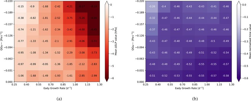
P. Besson et al.: Cyclone dry-dynamic forcing, deepening and propagation                                                           999

Figure 5. Cyclone-centred composites of upper-level QGω (in Pa s−1 ) during the growth phase (−1 < tnorm < 0) for the four forcing cate-
gories: (a) Q↑E↓, (b) Q↑E↑, (c) Q↓E↓, and (d) Q↓E↑. The black dot represents the cyclone centre (SLP minimum). Additionally, contour
lines of upper-level PV (in pvu) on the 320 K isentrope are shown.

level flow. Finally, near normalized time 0, both forcing fac-        located exactly above the surface cyclone centre; i.e. the
tors steeply decrease, which, of course, makes sense since            whole flow situation is nearly barotropic and hence indicates
the cyclone has already reached its mature stage and starts to        that only further weak cyclone deepening can be expected.
decay for times larger than 0. Figure S5 relates the normal-          This is in agreement with the deepening rates in Fig. 3a, and
ized time to the “real” mean time in hours before maximum             it also fits well to the normalized times in Fig. 3b, which
intensity in order to give some context to the dimensionless          now are outside the time window where the strongest deepen-
normalized time. Moreover, Fig. 4 shows that EGR values are           ing rates are expected (tnorm > −0.5). In accordance with the
dispersed only within a rather narrow range of values ( 0.67–         structure of the upper-level PV, QGω exhibits a rather sym-
0.9 d−1 ), while QGω values assume a much broader range               metric dipole, with descent to the west, ascent to the east,
from −0.04 to −0.16 Pa s−1 during the life cycle.                     and the surface cyclone centre slightly shifted towards the
                                                                      ascending pole (Fig. 5a). This reflects how sensitive the forc-
3.3   Cyclone-centred composites                                      ing at the cyclone centre reacts to slight horizontal displace-
                                                                      ments. In this category, for example, the forcing of vertical
                                                                      motion occurs too far to the east of the cyclone centre, re-
In this section, we turn our attention to the immediate sur-
                                                                      sulting in weaker cyclone deepening than in category Q↑E↑
roundings of cyclones during their growth phase. This is
                                                                      (Fig. 5b). Finally, the EGR signal in this category at the cy-
done individually for each of the four forcing categories and
                                                                      clone position (Fig. 6a) is clearly weaker than for the E↑ cat-
for potential vorticity (PV) at 320 K, QGω forcing, and EGR
                                                                      egories. Enhanced values are found to the southwest of the
(Figs. 5 and 6).
                                                                      upper-level PV structure indicative of a local velocity max-
   Category Q↑E↓ (Fig. 5a) displays a strong upper-level PV
                                                                      imum (a jet streak), but at the cyclone centre EGR remains
signal of up to 2.5 pvu resembling the structure of an upper-
                                                                      rather small.
level PV cutoff. The upper-level PV maximum is essentially

https://doi.org/10.5194/wcd-2-991-2021                                                 Weather Clim. Dynam., 2, 991–1009, 2021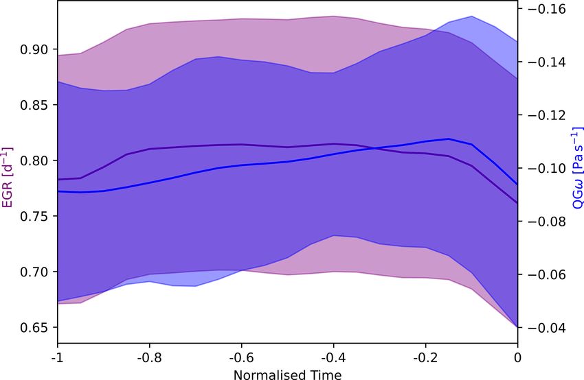
1000                                                 P. Besson et al.: Cyclone dry-dynamic forcing, deepening and propagation

Figure 6. As in Fig. 4, but for EGR (in 10−5 s−1 ). Grey arrows represent the wind field at 300 hPa.

   Category Q↑E↑ depicts the strongest upper-level PV sig-               EGR environment (Fig. 6c). Indeed, category Q↓E↓ exhibits
nal (Fig. 5b) among all four categories, with amplitudes                 the weakest deepening rates (Fig. 3a).
reaching up to 3.5 pvu and a rather pronounced horizontal                   A completely different upper-level PV structure is dis-
westward tilt of the upper-level PV maximum relative to the              cernible for category Q↓E↑ (Fig. 5d). The cyclone centre is
surface cyclone centre. It resembles a well-developed trough             located on the flank of a band of enhanced PV gradients ori-
located upstream of the surface cyclone centre, and it clearly           entated southwest to northeast. The cyclone is likely located
fits well into the conceptual model of a deepening cyclone in            near the exit of a jet streak that forms upstream around the
a PV framework (Hoskins et al., 1985). In accordance with                trough. This is in agreement with the existence of upper-level
the strong upper-level PV signal, a strong QGω dipole is dis-            QGω forcing (Fig. 5d) that is larger compared with Q↓E↓
cernible (Fig. 5b): with the surface cyclone located slightly            (Fig. 5c) but lower compared with Q↑E↓ (Fig. 5b). In this
to the south of the QGω maximum. The EGR maximum, on                     meteorological scenario we expect enhanced EGR forcing,
the other hand, is found to the southwest of the cyclone cen-            remembering that an upper-level jet by thermal wind balance
tre (Fig. 6b) where we expect the trailing surface cold front.           must be associated with a significant horizontal temperature
Given the strong forcing and the archetypal flow situation               gradient beneath its core and hence also with a correspond-
that is well known for many developing cyclones, it is no sur-           ing EGR signal by definition (see Sect. 2.1). Indeed, this can
prise that this category is characterized by the largest deep-           be seen in Fig. 6d. The normalized times associated with this
ening rates (as seen in Fig. 3a).                                        category (lower right in Fig. 3b) indicate that the cyclone de-
   Category Q↓E↓ displays a minor upper-level PV structure               velopment is rather in an early stage, as one would expect
(Fig. 5c), resembling a PV cutoff centred above the surface              from the upper-level PV structure that displays only a weakly
cyclone’s centre attaining only a small amplitude of 1.5 pvu.            developed trough and ridge.
The barotropic structure and small amplitude of the upper-
level PV points to small deepening rates, in particular to-
gether with a weak QGω forcing (Fig. 6c) and a uniform low-

Weather Clim. Dynam., 2, 991–1009, 2021                                                       https://doi.org/10.5194/wcd-2-991-2021
P. Besson et al.: Cyclone dry-dynamic forcing, deepening and propagation                                                                  1001

Figure 7. Wind rose plots showing the frequency (in percentage) of angle values for all 6 h track sections for different degrees of 12 h cyclone
deepening rates: (a) 1SLP values below −10 hPa, (b) 1SLP values between −10 and −6.5 hPa, (c) 1SLP values between −6.5 and −3 hPa,
and (d) 1SLP values between −3 and 0 hPa.

4   Dry-dynamic forcing, deepening rates, and                             4.1    Propagation angle and deepening rates
    propagation direction

While the previous section solely focused on the deepening                Figure 7 shows four different wind roses for varying deep-
rates of extratropical cyclones, consideration is now given to            ening rate regimes by means of the 12-hourly SLP changes.
the connection between the dry-dynamic forcing, the deep-                 For example, Fig. 7a consists of propagation angles corre-
ening rates, and the direction of propagation of the cyclone              sponding to time steps with deepening rates of 10 hPa 12 h−1
during its growth phase. The propagation direction at a time              or more. The rings indicate the frequency of a specific an-
instance along a track is determined by taking the cyclone’s              gle range (i.e. the wind rose petal). For instance, Fig. 7a in-
6 h displacement vector and determining the angle between                 cludes several petals, the longest of which points in the north-
this vector and a zonal vector; i.e. an angle 0 corresponds to            eastern direction or 45◦ . The corresponding petal reaches the
eastward propagation and 90◦ to northward propagation.                    outer ring of the plot, indicating that 34.2 % of all cyclones
                                                                          that deepen at a rate of 10 hPa 12 h−1 or less propagate into

https://doi.org/10.5194/wcd-2-991-2021                                                      Weather Clim. Dynam., 2, 991–1009, 2021
1002 P. Besson et al.: Cyclone dry-dynamic forcing, deepening and propagation Figure 8. Mean propagation angles (in degrees) in extended winter (October–March), averaged over a 500 km radius. Positive values (blue) correspond to poleward propagation and negative ones (red) to equatorward propagation. Additionally, four regions with distinct propagation signals are outlined by black boxes, and the distributions of propagation angles for all cyclones passing the region are shown, complemented by a Gaussian fit as a red line. The green contours represent eddy kinetic energy (10 d low-pass filter) at the 500 hPa level and provide the extent and intensity of the storm tracks. the northeastern direction. Therefore, the number and size agation in their lee (in agreement with the formation of sta- of the wind rose petals indicate the relationship between the tionary lee troughs). cyclone deepening and the direction of propagation. The re- A tendency for poleward propagation is characteristic for sults for weaker deepening (−10 hPa < 1SLP < −6.5 hPa) the North Atlantic and North Pacific storm tracks. It is strik- (Fig. 7b) indicate a dominant northeast-oriented propagation ing, and in agreement with earlier studies (Gilet et al., 2009; direction although the east-northeast petal is longer than in Rivière et al., 2012; Tamarin and Kaspi, 2016), how the re- Fig. 7a. For even weaker deepening (−6.5 hPa < 1SLP < gion of maximum deepening in the two oceanic basins co- −3 hPa) (Fig. 7c), most of the values are also within the incides with local maxima in mean poleward propagation northeastern direction; however, the largest petal is found in angles. Downstream of these maxima, in particular for the the east-northeast section (Fig. 7c). Moreover, the petal in the North Atlantic storm track, the poleward tendencies steadily eastern direction, for these weaker deepening rates, is signif- decrease, and over Europe the tendencies attain rather zonal icantly larger than in Fig. 7a and b. Finally, a shift toward values. Besides the storm track regions, additional distinct re- zonal (eastward) propagation angles is found for the weakest gions exhibit positive mean propagation angles: for instance, deepening rates (−3 hPa < 1SLP < 0 hPa) (Fig. 7d), where over California to the west of the Rocky Mountains, to the the two petals in the east and east-northeastern directions are east of Greenland, over the Black Sea, to the east of Lake the most prominent ones, each representing approximately Baikal, over northeast Siberia, and close to the Arctic Sea. 20 % of the angle values. Overall, we can summarize that It remains to be studied in a refined analysis to which de- while during their growth phase cyclones go through differ- gree these tendencies are determined by orographic effects ent magnitudes of deepening rates, during the times a cy- or other forcings. clone experiences higher deepening rates it tends to propa- Of course, as seen in the histograms of propagation angles gate more poleward. for the outlined four regions in Fig. 7, each region is charac- Next, consideration is given to the geographical distribu- terized by a rather wide spread of possible propagation an- tion of the direction of propagation. In Fig. 8 blue colours gles. For instance, in the North Pacific the mean propagation indicate a poleward propagation and red colours represent angle peaks near 45◦ , but smaller and higher values often oc- equatorward propagation. Areas with climatological equator- cur. Even higher northward propagation angles, in the mean, ward propagation are sparse and spatially confined to regions are found in the box over the western and central North At- downstream of mountain ranges, e.g. downstream of the Ti- lantic. This is in agreement with the fact that the North At- betan Plateau, leeward of the Himalayas, and over North lantic storm track is more tilted towards the northeast with in- America in the lee of the Rocky Mountains. Over Europe, creasing longitude compared to the North Pacific storm track equatorward propagation can be found leeward of the Alps. (Hoskins and Hodges, 2002; Wernli and Schwierz, 2006). Hence, mountain ranges are able to favour equatorward prop- Weather Clim. Dynam., 2, 991–1009, 2021 https://doi.org/10.5194/wcd-2-991-2021
P. Besson et al.: Cyclone dry-dynamic forcing, deepening and propagation 1003
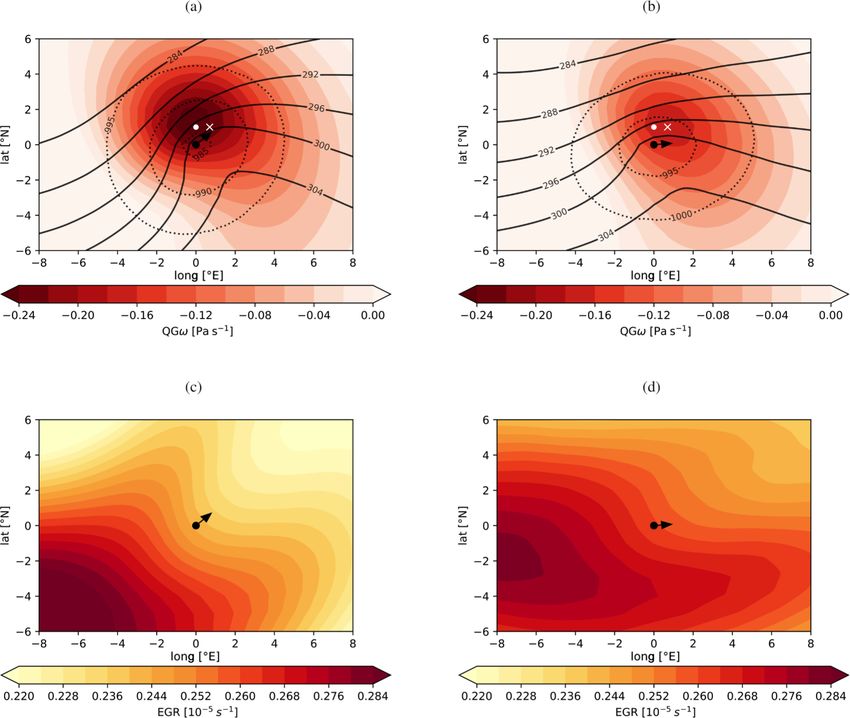
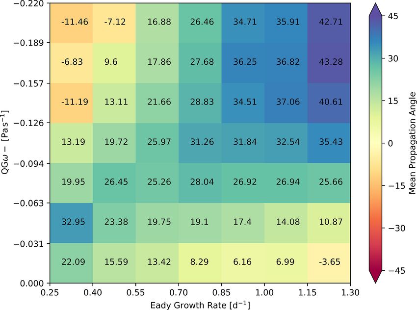
Figure 10 shows the QGω forcing (colour) for poleward-
propagating cyclones (Fig. 10a) and for cyclones propagating
more eastward (Fig. 10b). The categories are defined accord-
ing to a range of propagation angles: angles between 35 and
65◦ for poleward propagation and between −5◦ and 25◦ for
eastward propagation. The black dot represents the SLP min-
imum (cyclone centre), and the black arrow in the centre in-
dicates the mean propagation direction of the cyclone within
the following 6 h. To make the comparison easier, a white
point in both fields indicates the position of the maximum
QGω forcing for poleward propagation, and a white cross in-
dicates the maximum in the case of an eastward propagation.
In both cases, the cyclone centre is located close to and
just equatorward of the maximum QGω forcing. The maxi-
mum forcing is more pronounced for poleward-propagating
cyclones with values exceeding −0.24 Pa s−1 (Fig. 10a). The
Figure 9. The 2D forcing histogram as in Fig. 3a but depicting the
QGω maximum for eastward-propagating cyclones reaches
mean propagation angle in colour (in degrees; positive toward the
−0.16 Pa s−1 (Fig. 10b). The forcing in a case of poleward
poles, negative toward the Equator) against QGω forcing (Pa s−1 )
and Eady growth rate (d−1 ). propagation by QGω is purely poleward, and the direction
of propagation is northeastward (black arrow in Fig. 10a). In
contrast, for eastward-propagating cyclones the maximum of
4.2 2D forcing diagram for cyclone propagation QGω forcing (white cross) is not only weaker but also lo-
cated to the northeast of the cyclone centre, resulting in a
To determine the relationship between the dry-dynamic forc- more zonal direction of propagation. In summary, it seems
ing (QGω and EGR) and the direction of propagation, a his- that the weaker amplitude and eastward-shifted QGω centre
togram similar to the one in Fig. 3a is computed (Fig. 9). The lead to a more zonal cyclone propagation, whereas a QGω
first noticeable characteristic of the histogram is the fact that maximum to the north is able to deflect the cyclone path pole-
the upper right corner displays the strongest poleward propa- ward.
gation direction under strong dry-dynamic forcing. This was The EGR environment for poleward and zonal cyclone
also the corner with the highest 12 h 1SLP deepening rates propagation is shown in Fig. 10c and d. In the case of
(Fig. 3a) and a normalized time near and prior to the phase poleward-propagating cyclones (Fig. 10c), the displacement
with the deepest SLP (Fig. 3b). The cyclone is thus deepen- vector is orientated essentially normal to the EGR field,
ing most strongly while propagating poleward. If only one pointing towards lower EGR values. This indicates that cy-
forcing factor is high, either EGR (lower right) or QGω (up- clones propagate away from high EGR values, which are
per left), the cyclone seems to be in a period during its growth found in this case in the southwestern sector of the cyclone
phase that favours near zonal (eastward) or even slight equa- where one would expect the associated cold front to be lo-
torward propagation. Interestingly, if both forcing factors are cated. On the other hand, in the case of eastward-propagating
weak (lower left corner), a tendency for poleward propaga- cyclones (Fig. 10d), the displacement vector is also locally
tion is discernible, although the propagation angle remains normal to the EGR isolines, but the large-scale EGR envi-
lower than for the case of combined strong forcing. One rea- ronment has a stronger zonal orientation compared to the
son for this observation might be that cyclones which prop- poleward-propagating case. It is, however, difficult to judge
agated poleward under strong dry-dynamic forcing continue what the exact contribution by the EGR environment is to the
to do so even after both forcings have vanished. cyclone’s propagation.
4.3 Cyclone-centred composites for poleward and
eastward propagation 5 Conclusions
In the previous section, we saw that there is a general rela- The deepening and propagation of extratropical cyclones oc-
tionship between the deepening and the propagation of cy- curs within a remarkably wide range of environments. In
clones. Cyclones tend to propagate poleward when the deep- this study, we analysed the environment during the cyclone
ening is strongest. In this section, we link this result back growth period in terms of the dry-dynamic forcing, its vari-
to the dry-dynamic forcing QGω and EGR by means of ability, and its relationship with the cyclone propagation di-
cyclone-centred composites for cyclones that propagate pre- rection. To this aim, extratropical surface cyclones were iden-
dominantly poleward compared to eastward-propagating cy- tified and tracked during the Northern Hemisphere cold sea-
clones. son (October to March) based on 6-hourly ERA-Interim data
https://doi.org/10.5194/wcd-2-991-2021 Weather Clim. Dynam., 2, 991–1009, 20211004 P. Besson et al.: Cyclone dry-dynamic forcing, deepening and propagation
Figure 10. Cyclone-centred composites of QGω (coloured contours in Pa s−1 ) for (a) poleward-propagating cyclones (35◦ < α < 65◦ ) and
(b) eastward-propagating (−5◦ < α < 25◦ ) cyclones and EGR composites (coloured contours in 10−5 s−1 ) for (c) poleward-propagating
cyclones and (d) eastward-propagating cyclones. The black dot represents the cyclone centre and the arrow the mean 6 h propagation direction
of the cyclone. The white dot in (a) and (b) indicates the maximum of the QGω forcing for poleward-propagating cyclones and the white
cross the QGω maximum for eastward-propagating cyclones; i.e. they mark the exact location of colour-shaded QGω fields. The white dot
and cross are depicted in both (a) and (b) to highlight the spatial shift between the two forcing maxima. The black contour lines in (a) and
(b) show θe (in K) at 850 hPa, and the dotted lines show SLP (in hPa).
(1979–2016). Each time step along every cyclone track was within 12 h is found for a forcing of EGR = 1.3 d−1 and
characterized in terms of its 12 h deepening rate (1SLP), QGω = −0.22 Pa−1 . The second largest mean deepen-
the upper-level QG forcing for ascent (QGω), the lower- ing rates are found for category Q↓E↑ (−3 hPa within
tropospheric Eady growth rate (EGR), and the propagation 12 h for EGR = 1.3 d−1 and QGω = 0 Pa−1 ), followed
direction. Since cyclone deepening and direction of propaga- by Q↓E↓ and Q↑E↓.
tion are determined by a cyclone’s large-scale environment,
the QGω and EGR forcings were averaged within a 1000 km – An interesting asymmetry is discernible between condi-
radius around the cyclone centre. To facilitate the comparison tions with high EGR and low QGω forcings and, con-
between the multitude of cyclone tracks, the phase of the cy- versely, low EGR and high QGω forcings: larger deep-
clone evolution was quantified by introducing a normalized ening rates result for the former than the latter. This in-
time axis, with −1 corresponding to genesis, 0 to the time dicates that baroclinic instability and substantial deep-
instance of the deepest sea-level pressure (SLP), and +1 to ening rates can result even in situations with moderate
lysis. The analysis was restricted to the growth period of the upper-level (QGω) forcing as long as the EGR is high
life cycle between normalized times −1 and 0. The main re- enough. The opposite is, however, not true: even sub-
sults of the presented analysis can be summarized as follows. stantial upper-level forcing results only in weak deep-
ening rates if EGR is low.
– The largest 12 h deepening rates result for a combina-
tion of high EGR and strong QGω forcing (category – The four different forcing categories dominate differ-
Q↑E↑), as expected and clearly visualized in the forcing ent periods of the growth phase. The early phase clos-
histogram. For instance, a mean deepening rate of 6 hPa est to genesis is dominated by Q↓E↑, while thereafter
Weather Clim. Dynam., 2, 991–1009, 2021 https://doi.org/10.5194/wcd-2-991-2021You can also read