Inferring potential landslide damming using slope stability, geomorphic constraints, and run-out analysis: a case study from the NW Himalaya
←
→
Page content transcription
If your browser does not render page correctly, please read the page content below
Earth Surf. Dynam., 9, 351–377, 2021
https://doi.org/10.5194/esurf-9-351-2021
© Author(s) 2021. This work is distributed under
the Creative Commons Attribution 4.0 License.

               Inferring potential landslide damming using slope
                 stability, geomorphic constraints, and run-out
                  analysis: a case study from the NW Himalaya
                        Vipin Kumar1 , Imlirenla Jamir2 , Vikram Gupta3 , and Rajinder K. Bhasin4
                   1 Georisks   and Environment, Department of Geology, University of Liege, Liège, Belgium
                                2 CSIR – National Geophysical Research Institute, Hyderabad, India
                                     3 Wadia Institute of Himalayan Geology, Dehradun, India
                                         4 Norwegian Geotechnical Institute, Oslo, Norway

                                   Correspondence: Vipin Kumar (v.chauhan777@gmail.com)

                                Received: 5 September 2020 – Discussion started: 28 September 2020
                           Revised: 7 February 2021 – Accepted: 13 March 2021 – Published: 23 April 2021

       Abstract. Prediction of potential landslide damming has been a difficult process owing to the uncertainties
       related to landslide volume, resultant dam volume, entrainment, valley configuration, river discharge, material
       composition, friction, and turbulence associated with material. In this study, instability patterns of landslides,
       geomorphic indices, post-failure run-out predictions, and spatio-temporal patterns of rainfall and earthquakes are
       explored to predict the potential landslide damming sites. The Satluj valley, NW Himalaya, is chosen as a case
       study area. The study area has witnessed landslide damming in the past and incurred losses of USD ∼ 30 million
       and 350 lives in the last 4 decades due to such processes. A total of 44 active landslides that cover a total
       ∼ 4.81 ± 0.05 × 10⁶ m2 area and ∼ 34.1 ± 9.2 × 10⁶ m3 volume are evaluated to identify those landslides that
       may result in potential landslide damming. Out of these 44, a total of 5 landslides covering a total volume of
       ∼ 26.3 ± 6.7 × 10⁶ m3 are noted to form the potential landslide dams. Spatio-temporal variations in the pattern
       of rainfall in recent years enhanced the possibility of landslide triggering and hence of potential damming. These
       five landslides also revealed 24.8 ± 2.7 to 39.8 ± 4.0 m high debris flows in the run-out predictions.

1   Introduction                                                    (i) pre- and post-failure behaviour of landslide slopes and the
                                                                    (ii) landslide volume, stream power, and morphological set-
Landslide damming is a normal geomorphic process in nar-            ting of the valley (Kumar et al., 2019a).
row river valleys and poses significant natural hazard (Dai            To understand the pre-failure pattern, finite element
et al., 2005; Gupta and Sah, 2008; Delaney and Evans, 2015;         method (FEM)-based slope stability evaluation has been
Fan et al., 2020). Many studies have explored damming char-         among the most widely used approaches for complex slope
acteristics (Li et al., 1986; Costa and Schuster, 1988; Taka-       geometry (Griffiths and Lane, 1999; Jing, 2003; Jamir et al.,
hashi and Nakawaga, 1993; Ermini and Casagli, 2002; Fuji-           2017; Kumar et al., 2018). However, the selection of input
sawa et al., 2009; Stefanelli et al., 2016; Kumar et al., 2019a).   parameters in FEM analysis and the set of assumptions used
However, studies concerning the prediction of potential land-       (material model, failure criteria, and convergence) may also
slide dams and their stability at a regional scale have been        result in uncertainty in the final output (Wong, 1984; Cho,
relatively rare, particularly in the Himalaya despite a his-        2007; Li et al., 2016). Uncertainty from input parameters can
tory of landslide damming and flash floods (Gupta and Sah,          be resolved by performing parametric analysis, whereas the
2008; Ruiz-Villanueva et al., 2016; Kumar et al., 2019a). In        utilization of the most appropriate criteria can minimize the
order to identify the landslides that have the potential to form    uncertainty caused by assumptions. Post-failure behaviour of
dams, the following factors have been main prerequisites:           landslides can be understood using run-out analysis (Hungr

Published by Copernicus Publications on behalf of the European Geosciences Union.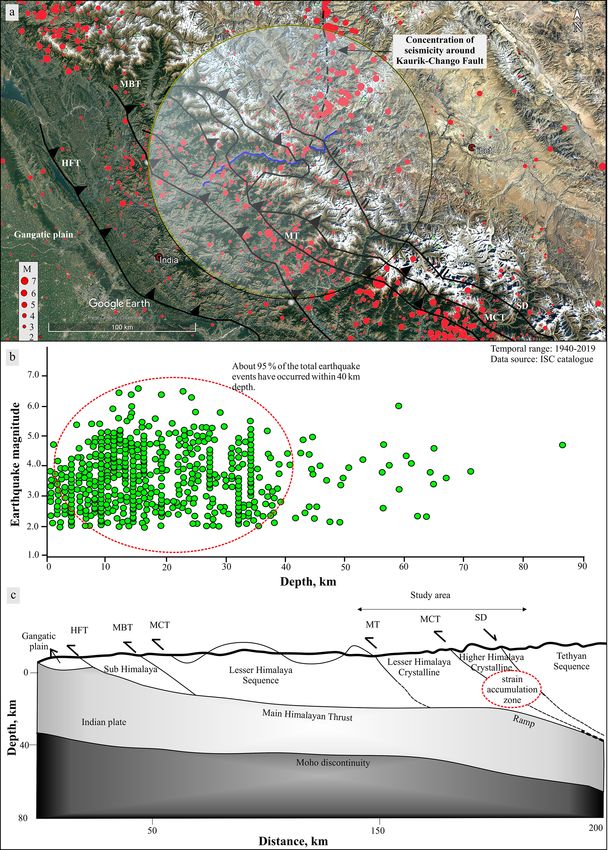
352                                                V. Kumar et al.: Inferring potential landslide damming using slope stability

et al., 1984; Hutter et al., 1994; Rickenmann and Scheidl,         2   Study area
2013). These methods could be classified into empirical or
statistical and dynamical categories (Rickenmann, 2005).           The study area is located between Moorang (31◦ 360 100 N,
Owing to the flexibility in rheology, solution approach, refer-    78◦ 260 4700 E) and Rampur (31◦ 270 1000 N, 77◦ 380 2000 E) in the
ence frame, and entrainment, dynamic models have been rel-         Satluj River valley, NW Himalaya (Fig. 1). The Satluj River
atively more realistic for site-specific problems (Corominas       flows across the Tethyan Sequence (TS), Higher Himalaya
and Mavrouli, 2011). Though the different numerical models         Crystalline (HHC), Lesser Himalaya Crystalline (LHC), and
have different advantages and limitations, Voellmy rheology-       Lesser Himalaya Sequence (LHS). The TS in the study area
based (friction and turbulence) (Voellmy, 1955; Salm, 1993)        is comprised of slate or phyllite and schist and has been in-
rapid mass movement simulation (RAMMS) (Christen et al.,           truded by the biotite-rich granite, i.e. Kinnaur Kailash Gran-
2010) has been used widely owing to the inclusion of rheo-         ite (KKG), near the Sangla Detachment (SD) fault (Sharma,
logical and entrainment rate flexibility.                          1977; Vannay et al., 2004). The SD fault separates the TS
   Apart from the pre- and post-failure pattern, landslide vol-    from the underlying crystalline rock mass of the HHC.
ume, stream power, and morphological setting of the val-           Migmatitic gneiss marks the upper part of the HHC, whereas
ley are crucial to infer the potential landslide damming.          the base is marked by the kyanite–sillimanite gneiss rock
The Morphological Obstruction Index (MOI) and Hydro-               mass (Sharma, 1977; Vannay et al., 2004; Kumar et al.,
morphological Dam Stability Index (HDSI) have been                 2019b). The Main Central Thrust (MCT) fault separates the
widely used as geomorphic indices to infer the potential of        HHC from the underlying schist and gneissic rock mass of
landslide dam formation and their temporal stability (Costa        the LHC. The LHC comprises mica schist, carbonaceous
and Schuster, 1988; Ermini and Casagli, 2002; Stefanelli et        schist, quartzite, and amphibolite. A thick zone of gneiss, i.e.
al., 2016).                                                        Wangtu Gneissic Complex (WGC), is exposed in the LHC,
   The NW Himalaya has been one of most landslide-                 which is comprised of augen gneiss and porphyritic gran-
affected terrains owing to the active tectonics and multiple       itoids. The LHC is delimited at the base by the Munsiari
precipitation sources, i.e. the Indian summer monsoon (ISM)        Thrust (MT) fault that is thrusted over the Lesser Himalaya
and western disturbance (Dimri et al., 2015; Jamir et al.,         Sequence (LHS) rock mass. The MT contains breccia, cata-
2019). The NW Himalaya accommodated ∼ 51 % of all the              clastic, and fault gouge (Sharma, 1977; Vannay et al., 2004;
landslides in India during the years 1800–2011 (Parkash,           Kumar et al., 2019b). The LHS in the study area consists
2011). The Satluj River valley, NW Himalaya, is one such           of quartz arenite (Rampur Quartzite) with bands of phyllite,
region where landslides and associated floods have claimed         meta-volcanics, and paragneiss (Sharma, 1977).
∼ 350 lives and resulted in the loss of minimum USD 30 mil-           The present study covers 44 active landslides (20 debris
lion in the last 4 decades. This region holds a high poten-        slides, 13 rockfalls, and 11 rock avalanches) along the study
tial for future landslide damming and resultant floods (Ruiz-      area (Table 1) that have been mapped recently by Kumar et
Villanueva et al., 2016; Kumar et al., 2019a). Therefore, the      al. (2019b). Field photographs of some of these landslides
Satluj valley is used here as a case study area, and 44 active     are presented in Fig. 2. The TS and LHS in the study area
landslides belonging to the different litho-tectonic regimes       have been subjected to relative tectonic tranquility with ex-
are modelled using the FEM technique. Multiple slope sec-          humation rates as low as 0.5–1.0 mm yr−1 , whereas the HHC
tions and a range of values of different input parameters are      and LHC region have undergone a 1.0–4.5 mm yr−1 rate of
used to perform the parametric study. In order to determine        exhumation (Thiede et al., 2009). The MCT fault region and
the human population that might be affected by these land-         the WGC are noted to have a maximum exhumation rate (i.e.,
slides, census statistics are also used. The MOI and HDSI are      ∼ 4.5 mm yr−1 ) that is evident from the deep gorges in these
used to determine the potential of landslide dam formation         regions (Fig. 2c and e). A majority of the earthquake events
and their stability, respectively. In view of the role of rain-    in the study area in the last 7 decades have been related to
fall and earthquakes as the main landslide-triggering factors,     the N–S oriented Kaurik–Chango fault (KCF) (Kundu et al.,
the spatio-temporal regime of these two factors is also dis-       2014; Hazarika et al., 2017; http://www.isc.ac.uk/iscbulletin/
cussed. Run-out prediction of certain landslides is also per-      search/catalogue/, last access: 2 March 2020). The climate
formed to understand the role of run-out in potential land-        in the study area shows a spatial variation, from humid
slide damming. This study provides detailed insight into the       (∼ 800 mm yr−1 mean annual precipitation) in the LHS to
regional instability pattern, associated uncertainty, and po-      semi-arid (∼ 200 mm yr−1 ) in the TS (Kumar et al., 2019b).
tential landslide damming sites, and hence it can be repli-        The HHC acts as a transition zone where climate varies from
cated in other hilly terrain that witnesses frequent landslides    semi-humid to semi-arid in the SW–NE direction. This tran-
and damming.                                                       sition has been attributed to the “orographic barrier” nature
                                                                   of the HHC that marks the region in its north as “orographic
                                                                   interior” and the region to its south as the “orographic front”
                                                                   (Wulf et al., 2012; Kumar et al., 2019b).

Earth Surf. Dynam., 9, 351–377, 2021                                                  https://doi.org/10.5194/esurf-9-351-2021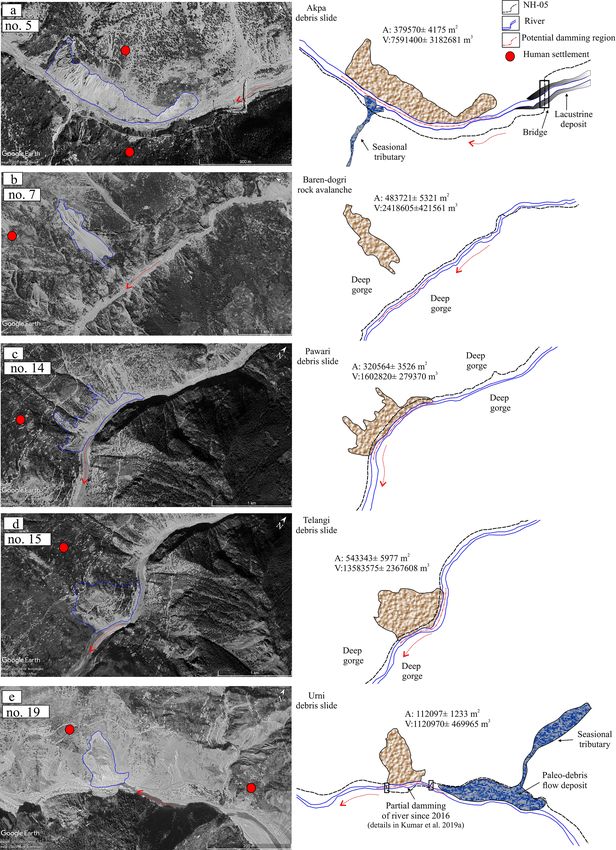
V. Kumar et al.: Inferring potential landslide damming using slope stability                                                            353

Table 1. Details of the landslides used in the study.

   Serial no.   Landslide      Latitude/          Type                   Areaa , m2            Volumeb , m3        Human     Litho-
                location       longitude                                                                       populationc   tectonic
                                                                                                                             division
   1            Khokpa         31◦ 350 18.900 N   Debris slide        21 897 ± 241          43 794 ± 18 361           373    Tethyan
                               78◦ 260 28.600 E                                                                              sequence
   2            Tirung Khad    31◦ 340 50.400 N   Rockfall            28 537 ± 314            14 269 ± 9055             0    (TS)
                               78◦ 260 20.500 E
   3            Akpa_I         31◦ 340 57.100 N   Rock             963 051 ± 10 594     1 926 102 ± 807 515             0    TS-KKG
                               78◦ 240 30.600 E   avalanche
   4            Akpa_II        31◦ 350 2.200 N    Rock               95 902 ± 1055         143 853 ± 40 734           470    Kinnaur
                               78◦ 230 25.400 E   avalanche                                                                  Kailash
   5            Akpa_III       31◦ 340 54.500 N   Debris slide      379 570 ± 4175     7 591 400 ± 3 182 681         1617    Granite
                               78◦ 230 2.400 E                                                                               (KKG)
   6            Rarang         31◦ 350 58.700 N   Rockfall               4586 ± 50             4586 ± 1923            848    Higher
                               78◦ 200 39.100 E                                                                              Himalaya
   7            Baren Dogri    31◦ 360 23.600 N   Rock              483 721 ± 5321      2 418 605 ± 421 561           142    Crystalline
                               78◦ 200 23.100 E   avalanche                                                                  (HHC)
   8            Thopan         31◦ 360 12.300 N   Rockfall            55 296 ± 608         165 888 ± 46 974           103
                Dogri          78◦ 190 50.400 E
   9            Kashang        31◦ 360 5.000 N    Debris slide      113 054 ± 1244         169 581 ± 48 019           103
                Khad_I         78◦ 180 44.400 E
   10           Kashang        31◦ 350 58.300 N   Rockfall            27 171 ± 299          40 757 ± 11 541           103
                Khad_II        78◦ 180 34.000 E
   11           Pangi_I        31◦ 350 36.400 N   Debris slide        30 112 ± 331          45 168 ± 12 790          1389
                               78◦ 170 36.400 E
   12           Pangi_II       31◦ 350 38.900 N   Debris slide         59436 ± 654         118 872 ± 49 837          1389
                               78◦ 170 12.200 E
   13           Pangi_III      31◦ 340 38.900 N   Debris slide        75 396 ± 829         188 490 ± 32 854             7
                               78◦ 160 55.600 E
   14           Pawari         31◦ 330 49.800 N   Debris slide      320 564 ± 3526      1 602 820 ± 279 370          4427
                               78◦ 160 28.600 E
   15           Telangi        31◦ 330 7.000 N    Debris slide       543 43 ± 5977    13 583 575 ± 2 367 608         6817
                               78◦ 160 37.200 E
   16           Shongthong     31◦ 310 13.000 N   Debris slide           5727 ± 63            11 454 ± 2464           388
                               78◦ 160 17.000 E
   17           Karchham       31◦ 300 12.400 N   Rock avalanche      28 046 ± 309          56 092 ± 23 516             0
                               78◦ 110 30.800 E
   18           Choling        31◦ 310 17.000 N   Debris slide        20 977 ± 231            20 977 ± 8795             0    Lesser
                               78◦ 80 4.900 E                                                                                Himalaya
   19           Urni           31◦ 310 8.000 N    Debris slide      112 097 ± 1233      1 120 970 ± 469 965           500    Crystalline
                               78◦ 70 42.200 E    (LHC)
   20           Chagaon_I      31◦ 300 55.900 N   Rockfall               3220 ± 35             3220 ± 1350              0
                               78◦ 60 52.000 E
   21           Chagaon_II     31◦ 300 57.900 N   Rockfall            11 652 ± 128            11 652 ± 4885             0
                               78◦ 60 47.700 E
   22           Chagaon_III    31◦ 310 3.000 N    Debris slide         42141 ± 464         168 564 ± 70 670          1085
                               78◦ 60 21.400 E

https://doi.org/10.5194/esurf-9-351-2021                                                       Earth Surf. Dynam., 9, 351–377, 2021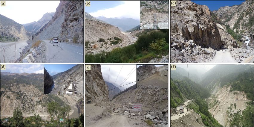
354                                                                    V. Kumar et al.: Inferring potential landslide damming using slope stability

Table 1. Continued.

       Serial no.       Landslide           Latitude/              Type                          Areaa , m2              Volumeb , m3             Human           Litho-
                        location            longitude                                                                                         populationc         tectonic
                                                                                                                                                                  division
       23               Wangtu_U/s          31◦ 320 4.800 N        Rock avalanche          211 599 ± 2328           317 399 ± 89 876                      17      Lesser
                                            78◦ 30 5.000 E                                                                                                        Himalaya
       24               Wangtu              31◦ 330 27.700 N       Debris slide                   4655 ± 51               9310 ± 3903                     71      Crystalline
                        D/s_1               77◦ 590 43.700 E
       25               Kandar              31◦ 330 43.700 N       Rock                    151 128 ± 1662          302 256 ± 126 720                     186
                                            77◦ 590 54.900 E       avalanche
       26               Wangtu              31◦ 330 38.900 N       Debris slide                   8004 ± 88             16 008 ± 6711                     71
                        D/s_2               77◦ 590 29.900 E
       27               Agade               31◦ 330 52.300 N       Debris slide                 9767 ± 107              14 651 ± 4149                    356
                                            77◦ 580 3.500 E
       28               Punaspa             31◦ 330 37.600 N       Debris slide                   3211 ± 35               3211 ± 1346                    343
                                            77◦ 570 31.500 E
       29               Sungra              31◦ 330 58.800 N       Debris slide                   5560 ± 61             11 120 ± 4662                  2669
                                            77◦ 560 49.600 E
       30               Chota               31◦ 330 39.200 N       Rock                    197 290 ± 2170          591 870 ± 167 597                     401
                        Kamba               77◦ 540 39.000 E       avalanche
       31               Bara Kamba          31◦ 340 10.400 N       Rockfall                   36 347 ± 400              18 174 ± 7619                    564
                                            77◦ 520 56.700 E
       32               Karape              31◦ 330 44.900 N       Debris slide               50 979 ± 561            50 979 ± 21 373                  1118
                                            77◦ 530 13.900 E
       33               Pashpa              31◦ 340 40.200 N       Rockfall                   16 079 ± 171                8040 ± 3371                     29
                                            77◦ 500 53.000 E
       34               Khani               31◦ 330 43.400 N       Rock                    218 688 ± 2406          874 752 ± 366 738                        0
                        Dhar_I              77◦ 480 52.500 E       avalanche
       35               Khani               31◦ 330 26.300 N       Rock                    146 994 ± 1617          734 970 ± 248 125                        0
                        Dhar_II             77◦ 480 35.800 E       avalanche
       36               Khani               31◦ 330 20.100 N       Rock                       20 902 ± 230            62 706 ± 17 756                       0
                        Dhar_III            77◦ 480 27.800 E       avalanche
       37               Jeori               31◦ 310 58.800 N       Rock                     93 705 ± 1031             93 705 ± 39 286                       0
                                            77◦ 460 18.200 E       avalanche
       38               Barauni             31◦ 280 56.600 N       Debris slide               63 241 ± 696         758 892 ± 111 620                     236      LHC-LHS
                        Gad_I_S             77◦ 410 40.400 E
       39               Barauni             31◦ 290 00.000 N       Debris slide               59 273 ± 652         711 276 ± 104 616                        0     Lesser
                        Gad_I_Q             77◦ 410 38.000 E                                                                                                      Himalaya
       40               Barauni             31◦ 280 43.900 N       Rockfall                       6977 ± 77               3489 ± 1463                       0     Sequence
                        Gad_II              77◦ 410 24.600 E                                                                                                      (LHS)
       41               Barauni             31◦ 290 5.600 N        Rockfall                   33 115 ± 364            33 115 ± 13 883                       0
                        Gad_III             77◦ 410 23.700 E
       42               D/s Barauni         31◦ 280 24.900 N       Rockfall                   19 101 ± 210              19 101 ± 8008                       0
                        Gad_I               77◦ 410 8.400 E
       43               D/s Barauni         31◦ 280 25.500 N       Rockfall                   21 236 ± 234              21 236 ± 8903                       0
                        Gad_II              77◦ 400 56.700 E
       44               D/s Barauni         31◦ 280 7.400 N        Rockfall                   15 632 ± 172              15 632 ± 6554                       0
                        Gad_III             77◦ 400 42.400 E
      a Error (±) caused by GE measurement (1.06 %). b Error (±) is an outcome of multiplication of area ± error and thickness ± error. Thickness error (SD) corresponds to
      averaging of field-based approximated thickness. c The human population is based on the 2011 Govt. of India census. The villages and towns in the radius of 500 m from the
      landslide are considered for counting the human population.

Earth Surf. Dynam., 9, 351–377, 2021                                                                                      https://doi.org/10.5194/esurf-9-351-2021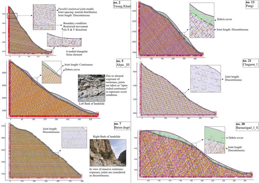
V. Kumar et al.: Inferring potential landslide damming using slope stability                                                             355

Figure 1. Geological setting. WGC stands for Wangtu Gneissic Complex. The dashed red circle in the inset (© Google Earth) represents
the region within a 100 km radius from the Satluj River (marked as a blue line) that was used to determine the earthquake distribution in the
area. Yellow lines represent the regional faults in the region. KCF in the inset refers to the Kaurik–Chango fault. The numbers 1–44 refer to
serial number of landslides in Table 1.

Figure 2. Field photographs of some of the landslides: (a) Khokpa landslide (no. 1), (b) Akpa_III landslide (no. 5), (c) Rarang land-
slide (no. 6), (d) Pawari landslide (no. 14), (e) Urni landslide (no. 19), and (f) Barauni Gad_I_S landslide (no. 38). The black circle in the
pictures that encircles the vehicle is intended to represent the relative scale.

https://doi.org/10.5194/esurf-9-351-2021                                                        Earth Surf. Dynam., 9, 351–377, 2021
356                                                V. Kumar et al.: Inferring potential landslide damming using slope stability

   Landslides in the study area have been a consistent threat      shear test (IS: 2720-Part 13-1986). If the soil samples con-
to the socio-economic condition of the nearby human pop-           tained < 5 % fines (< 75 mm), the hydrometer test was not
ulation (Gupta and Sah, 2008; Ruiz-Villanueva et al., 2016;        performed for the remaining fine material. In the direct shear
Kumar et al., 2019a). Therefore, the human population in the       test, soil samples were sheared under the constant normal
vicinity of each landslide was also determined by considering      stress of 50, 100, and 150 kN m−2 . The UCS test of soil was
the nearby villages and towns. Notably, a total of 25 822 peo-     performed under three different rates of movements, i.e. 1.25,
ple reside within 500 m extent of the 44 landslide slopes,         1.50, and 2.5 mm min−1 .
and about 70 % of this population is residing in the reach
of debris-slide-type landslides. Since the Government of In-       3.2   Slope stability modelling
dia keeps a 10-year gap in census statistics, the human pop-
ulation data was based on the most recent official data, i.e.      The finite element method (FEM) was used along with the
the census of 2011. The next official census is due in 2021.       shear strength reduction (SSR) technique to infer the critical
The population density in the Indian Himalayan region was          strength reduction factor (SRF), shear strain (SS), and total
estimated to be 181 per square kilometre in the year 2011          displacement (TD) in the 44 landslide slopes using the RS2
that might grow to 212 per square kilometre in 2021 with           software. The SRF has been observed to be similar in na-
a decadal growth rate of 17.3 % (https://censusindia.gov.in,       ture to the factor of safety (FS) of the slope (Zienkiewicz
last access: 2 September 2020; http://gbpihedenvis.nic.in,         et al., 1975; Griffiths and Lane, 1999). To define the fail-
last access: 2 September 2020).                                    ure in the SSR approach, non-convergence criteria were used
                                                                   (Nian et al., 2011). The boundary condition with the restrain-
                                                                   ing movement was applied to the base and back, whereas the
3     Methodology
                                                                   front face was kept free for the movement (Fig. 3). In situ
The methodology involved field data collection, satellite          field stress was adjusted in view of dominant stress, i.e. ex-
imagery analysis, laboratory analyses, slope stability mod-        tension or compression, by changing the value of the coeffi-
elling, geomorphic indices, rainfall and earthquake patterns       cient of earth pressure (k). A value of k = σh /σv = 0.5 was
and run-out modelling. Details are as follows.                     used in extensional regime, whereas k = σh /σv = 1.5 was
                                                                   used in compressional regime. The Tethyan Sequence has
                                                                   been observed to possess the NW–SE directed extensional
3.1    Field data, satellite imagery processing, and               regime. The structures in the upper part of the HHC are in-
       laboratory analyses                                         fluenced by the east directed extension along the SD fault.
The fieldwork involved rock and soil sample collection from        The lower part, however, is characterized by the SW-directed
each landslide location, rock mass joint mapping, and N-type       compression along the Main Central Thrust. In contrast to
Schmidt hammer rebound (SHR) measurement. Joints were              the HHC, structures in the Lesser Himalaya Crystalline and
included in the slope models for the FEM-based slope stabil-       Munsiari Thrust region are influenced by the compressional
ity analysis. The dataset involving the joint details is avail-    regime. In the Lesser Himalaya Sequence region, the SW-
able in the data repository (Kumar et al., 2021). The SHR          directed compressional regime has been observed on the ba-
values were obtained as per International Society of Rock          sis of the SW-verging folds, crenulation cleavage, and other
Mechanics (ISRM) standard (Aydin, 2008). Cartosat-1 satel-         features (Vannay et al., 2004).
lite imagery and field assessments were used to finalize the          The soil and rock mass were used in the models through
location of slope sections (2D) of the landslides. Cartosat-1      the Mohr–Coulomb (M–C) failure criterion (Coulomb, 1776;
imagery has been used widely for the landslide-related stud-       Mohr, 1914) and generalized Hoek–Brown (GHB) criterion
ies (Martha et al., 2010). The Cartosat-1 Digital Elevation        (Hoek et al., 1995), respectively. The parallel statistical dis-
Model (DEM) having 10 m spatial resolution, prepared using         tribution of the joints with normal distributed joint spacing in
the Cartosat-1 stereo imagery, was used to extract the slope       the rock mass was applied through the Barton–Bandis (B–B)
sections of the landslides using the Arc GIS-10.2 software.        slip criterion (Barton and Choubey, 1977; Barton and Bandis,
Details of the satellite imagery are mentioned in Table 2.         1990). Plane strain triangular elements that have six nodes
   The rock/soil samples were analysed in the National             were used through the graded mesh in the models. Details of
Geotechnical Facility (NGF) and Wadia Institute of Hi-             the criteria used in the FEM analysis are mentioned in Ta-
malayan Geology (WIHG) laboratory, India. The rock sam-            ble 3. The dataset of input parameters used in the FEM anal-
ples were drilled and smoothed for Unconfined Compressive          ysis is available in the data repository (Kumar et al., 2021). It
Strength (UCS) (IS: 9143-1979) and ultrasonic tests (CATS          is worth noting that the FEM analysis was performed under
Ultrasonic (1.95) of Geotechnical Consulting & Testing Sys-        the static load, i.e. field stress and body force. The dynamic
tems). The ultrasonic test was conducted to determine the          analysis was not performed at present due to the absence of
density, elastic modulus, and Poisson’s ratio of rock sam-         any major seismic events in the region in the last 4 decades
ples. The soil samples were tested for grain size (IS: 2720-       (Sect. 4.3) and lack of reliable dynamic load data of nearby
Part 4-1985), UCS test (IS: 2720-Part 10-1991), and direct         major seismic events.

Earth Surf. Dynam., 9, 351–377, 2021                                                  https://doi.org/10.5194/esurf-9-351-2021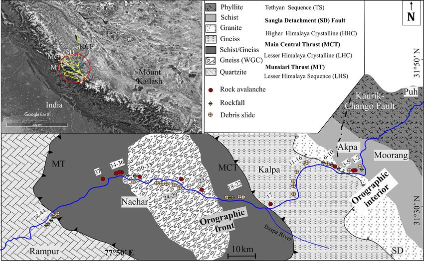
V. Kumar et al.: Inferring potential landslide damming using slope stability                                                             357

Table 2. Details of the satellite imagery.

                               Satellite data          Source                              Date of           Spatial
                                                                                           data            resolution
                        CARTOSAT-1           524/253   National Remote Sensing Center      5 Dec 2010       ∼ 2.5 m
                        stereo               525/253   (NRSC), Hyderabad, India            16 Dec 2010      ∼ 2.5 m
                        imagery              526/252                                       18 Oct 2011      ∼ 2.5 m
                                             526/253                                       18 Oct 2011      ∼ 2.5 m
                                             527/252                                       24 Nov 2010      ∼ 2.5 m
                                             527/253                                       27 Dec 2010      ∼ 2.5 m
                                             528/252                                       26 Nov 2011      ∼ 2.5 m

Figure 3. The FEM configuration of some of the slope models (no. refers to the serial no. of landslides in Table 1). The joint distribution in
all the slopes was parallel statistical with the normal distribution of joint spacing.

   To understand the uncertainty caused by the selection of              formed. In the parametric study for debris slides, the Akpa
2D slope section, multiple slope sections were taken wher-               landslide (no. 5 in Fig. 3), Pangi landslide (no. 13 in Fig. 3),
ever possible. More than one slope section was modelled                  and Barauni Gad landslide (no. 38 in Fig. 3) were chosen,
for each debris slide, whereas for the rockfalls or rock                 whereas the Tirung Khad (no. 2 in Fig. 3) and Chagaon land-
avalanches only one slope section was chosen due to the lim-             slides (no. 21 in Fig. 3) were considered to represent rockfall.
ited width of the rockfalls (or rock avalanches) in the study            The Baren Dogri (no. 7 in Fig. 3) landslide was used to rep-
area. To find out the relative influence of different input pa-          resent the rock avalanches. The selection of these landslides
rameters on the final output, a parametric study was per-                for the parametric study was based on the following two fac-

https://doi.org/10.5194/esurf-9-351-2021                                                        Earth Surf. Dynam., 9, 351–377, 2021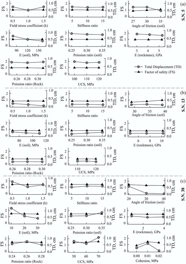
V. Kumar et al.: Inferring potential landslide damming using slope stability

                                                                                                                                                                                                                                    https://doi.org/10.5194/esurf-9-351-2021
                                                                               Table 3. Criteria used in the finite element method (FEM) analysis.
                                                                                                             Material criteria                                Parameters                 Source
                                                                                Rock mass     Hoek et al. (1995)                                              Unit weight, γ (MN m−3 )   Laboratory analysis (UCS)
                                                                                              σ1 = σ3 + σci [mb (σ3 /σci ) + s] ∧ a                           Uniaxial compressive       (IS: 9143-1979)
                                                                                                                                                              strength, σci (MPa)
                                                                                                                                                              Rock mass modulus          Laboratory analysis
                                                                                              Here, σ1 and σ3 are major and minor effective principal         (MPa)                      (Ultrasonic velocity test); Hoek
                                                                                              stresses at failure; σci , compressive strength of intact                                  and Diederichs (2006).
                                                                                              rock; mb , a reduced value of the material constant (mi ) and
                                                                                              is given by                                                     Poisson’s ratio
                                                                                              mb = mi e[(GSI−100)/(28−14D]                                    Geological strength        Field observation and based
                                                                                                                                                              index                      on recent amendments (Cai et al. , 2007,
                                                                                                                                                                                         and references therein)
                                                                                              s and a; constants for the rock mass given by the               Material constant          Standard values
                                                                                              following relationships:                                        (mi )                      (Hoek and Brown, 1997)
                                                                                              s = e[(GSI−100)/(9−3D] .
                                                                                                               GSI         20
                                                                                              a = 21 + 61 [e[−( 15 )] − e[−( 3 )] ]                           mb                         GSI was field-dependent, mi as

                                                                                                                                                                                                                                    Earth Surf. Dynam., 9, 351–377, 2021
                                                                                              Here, D is a factor which depends upon the degree of            s                          per Hoek and Brown (1997), and
                                                                                              disturbance to which the rock mass has been subjected by        a                          D is used between 0–1 in view
                                                                                              blast damage and stress relaxation. GSI (geological             D                          of rock mass exposure and
                                                                                              strength index) is a rock mass characterization parameter.                                 blasting.
358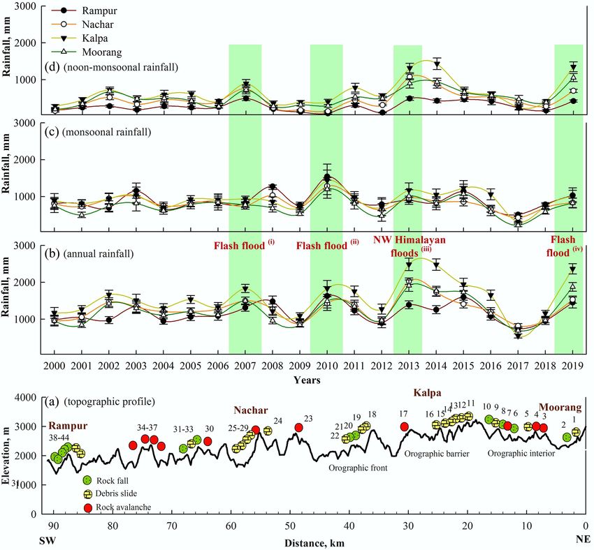
Table 3. Continued.

                                                                          Material criteria                               Parameters                Source
                                            Joint   Barton–Bandis Criteria                                                Normal stiffness, kn      Ei is lab-dependent. L and GSI
                                                    (Barton and Choubey, 1977; Barton and Bandis, 1990)                   (MPa m−1 )                were field-dependent. D is
                                                    τ = σn tan[∅r + JRClog10 (JCS/σn )]                                                             used between 0–1 in view of
                                                                                                                                                    rock mass exposure and blasting.
                                                    Here, τ is joint shear strength; σn , normal stress across joint;     shear stiffness, ks       It is assumed as kn /10.
                                                    ∅r , reduced friction angle; JRC, joint roughness                     (MPa m−1 )                However, the effect of the denominator
                                                    JCS, joint compressive strength.                                                                is also obtained through
                                                                                                                                                    parametric study.
                                                    JRC is based on the chart of Barton and Choubey (1977),               Reduced friction angle,   Standard values (Barton and
                                                    coefficient; Jang et al. (2014). JCS was determined using following   ∅r                        Choubey, 1977).
                                                    equation:
                                                    log10 (JCS) = 0.00088(RL )(γ ) + 1.01.

https://doi.org/10.5194/esurf-9-351-2021
                                                    Here, RL is Schmidt hammer rebound value and γ is                     Joint roughness           Field-based data from
                                                    unit weight of rock.                                                  coefficient, JRC          profilometer and standard
                                                    The JRC and JCS were used as JRCn and JCSn following                                            values from Barton and
                                                    the scale corrections observed by Barton and Choubey                                            Choubey (1977); Jang et al.
                                                    (1977) and references therein and proposed by Barton and                                        (2014).
                                                    Bandis (1982).
                                                                                                                          Joint compressive         Empirical equation of Deere and
                                                    JRCn = [JRC(L/L0 ){−0.02(JRC)} ]                                      strength, JCS (MPa)       Miller (1966) relating Schmidt
                                                    JCSn = [JCS(L/L0 ){−0.03(JRC)}                                                                  hammer rebound (SHR)
                                                    Here, land L0 are mean joint spacing in field                                                   values, σci , and unit weight of
                                                    L0 has been suggested to be 10 cm.                                                              rock. SHR was field-dependent.
                                                    Joint stiffness criteria                                              Scale corrected, JRCn     Empirical equation of Barton
                                                                                                                                                                                             V. Kumar et al.: Inferring potential landslide damming using slope stability

                                                    kn = (Ei · Em )/L · (Ei − Em )                                        Scale corrected, JCSn     and Bandis (1982).
                                                    (Barton, 1972)                                                        (MPa)
                                                    Here, kn ; Joint normal stiffness, Ei ; intact rock modulus,
                                                    Em ; rock mass modulus L; mean joint spacing.
                                                    Em = (Ei ) · [0.02 + {1 − D/2}/{1 + e(60+15·D−GSI)/11) }]
                                                    Here, Em is based on Hoek and Diederichs (2006) and
                                                    references therein
                                            Soil    Mohr–Coulomb criteria                                                 Unit weight               laboratory analysis (UCS)
                                                                                                                          (MN m−3 )                 (IS: 2720-Part 4–1985;
                                                                                                                                                    IS: 2720-Part 10-1991)
                                                    (Coulomb, 1776; Mohr, 1914)                                           Young’s Modulus, Ei       Laboratory analysis (UCS);
                                                    τ = C + σ tan ∅                                                       (MPa)                     IS: 2720-Part 10-1991.
                                                    Here, τ ; Shear stress at failure, C; Cohesion, σn ; normal           Poisson’s ratio           Standard values from Bowles
                                                    strength, ∅; angle of friction.                                                                 (1996)
                                                                                                                          Cohesion, C (MPa)         Laboratory analysis (Direct
                                                                                                                          Friction angle, ∅         shear)
                                                                                                                                                    (IS: 2720-Part 13-1986)

Earth Surf. Dynam., 9, 351–377, 2021
                                                                                                                                                                                             359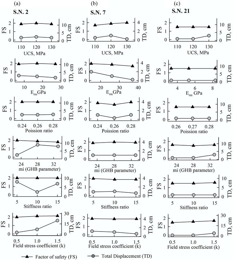
360                                                 V. Kumar et al.: Inferring potential landslide damming using slope stability

tors: (1) to choose the landslides from different litho-tectonic    four different locations: Moorang, Kalpa, Nachar, and Ram-
regime and (2) to represent varying stress regimes, i.e. ex-        pur (Locations mentioned in Fig. 1). The dataset of earth-
tensional, compressional, and relatively stagnant. The para-        quake events (2 < M < 8) in and around study area during
metric study of the debris slide models involved following          the years 1940–2019 was retrieved from the International
nine parameters: field stress coefficient, stiffness ratio, cohe-   Seismological Centre (ISC) catalogue (http://www.isc.ac.uk/
sion and angle of friction of soil, elastic modulus and Pois-       iscbulletin/search/catalogue/, last access: 2 March 2020) to
son’s ratio of soil, rock mass modulus, Poisson’s ratio, and        determine the spatio-temporal pattern.
uniaxial compressive strength of rock. For the rockfalls and
rock avalanches, the following six parameters were consid-          3.5   Run-out modelling
ered: uniaxial compressive strength of rock, rock mass mod-
ulus of rock, Poisson’s ratio of rock, “mi ” parameter, stiff-      Since the study area has witnessed many disastrous (mostly
ness ratio, and field stress coefficient. The “mi ” is a general-   rainfall-triggered) landslides and flash floods in past (Gupta
ized Hoek–Brown (GHB) parameter that is equivalent to the           and Sah, 2008; Ruiz-Villanueva et al., 2016), run-out anal-
angle of friction of Mohr–coulomb (M–C) criteria.                   ysis was performed to understand the post-failure scenario.
                                                                    Such run-out predictions will also be helpful to ascertain the
                                                                    possibility of damming because various studies have noted
3.3   Geomorphic indices
                                                                    river damming by the debris flows (Li et al., 2011; Braun et
Considering the possibility of landslide dam formation in the       al., 2018; Fan et al., 2020). The landslides that have potential
case of slope failure, the following geomorphic indices were        to form dams based on the indices (Sect. 3.3) are evaluated
also used:                                                          for such run-out analyses.
                                                                       In this study, a Voellmy rheology-based (Voellmy, 1955;
  i. Morphological Obstruction Index (MOI)                          Salm, 1993) rapid mass movement simulation (RAMMS)
                                                                    (Christen et al., 2010) model was used to understand the run-
      MOI = log (Vl /Wv ) ,                                  (1)
                                                                    out pattern. The RAMMS for debris flow uses the Voellmy
                                                                    friction law and divides the frictional resistance into a dry
 ii. Hydro-morphological Dam Stability Index (HDSI)                 Coulomb-type friction (µ) and viscous turbulent friction (ξ ).
      HDSI = log (Vd /Ab · S) ,                              (2)    The frictional resistance S (Pa) is

                                                                    SµN + ρgu2 /ξ,                                              (3)
where Vd (dam volume) = Vl (landslide volume, m3 ), Ab
is upstream catchment area (km2 ), Wv is width of the               where N = ρhg cos(φ) is the normal stress on the running
valley (m), and S is local slope gradient of river chan-            surface, ρ is density, g is gravitational acceleration, φ is slope
nel (m m−1 ). Though the resultant dam volume could be              angle, h is flow height, and u = (ux, uy) is the flow velocity
higher or lower than the landslide volume owing to slope            in the x and y directions. In this study, a range of friction (µ)
entrainment, rock mass fragmentation, retaining of material         and turbulence (ξ ) values, apart from other input parameters,
at the slope, and washout by the river (Hungr and Evans,            are used to evaluate the uncertainty in output (Table 4). Gen-
2004; Dong et al., 2011), dam volume is assumed to be               erally, the values for µ and ξ are determined using the re-
equal to landslide volume for the worst case. By utiliz-            construction of real events through the simulation and sub-
ing the comprehensive dataset of ∼ 300 landslide dams of            sequent comparison between the dimensional characteristics
Italy, Stefanelli et al. (2016) have classified the MOI into        of real and simulated events. However, the landslides in the
the (i) non-formation domain (MOI < 3.00), (ii) uncertain           study area merge with the river floor and/or are in close prox-
evolution domain (3.00 < MOI > 4.60), and (iii) formation           imity, and hence there is no failed material left from the pre-
domain (MOI > 4.60). By utilizing the same dataset, Ste-            vious events to reconstruct. Therefore, the µ and ξ values
fanelli et al. (2016) defined the HDSI into following cate-         were taken from a range in view of topography of landslide
gories (i) instability domain (HDSI < 5.74), (ii) uncertain de-     slope and run-out path, landslide material, similar landslide
termination domain (5.74 < HDSI > 7.44), and (iii) stability        events or materials, and results from previous studies and
domain (HDSI > 7.44).                                               models (Hürlimann et al., 2008; Rickenmann and Scheidl,
                                                                    2013; RAMMS v.1.7.0). Since these landslides are relatively
                                                                    deep in nature and happen during slope failure, irrespective
3.4   Rainfall and earthquake regime
                                                                    of type of trigger, and the entirety of the loose material might
Precipitation in the study area is related primarily to             not slide down, the depth of the landslide is taken as only
the Indian Summer Monsoon (ISM) and Western Distur-                 one-quarter (thickness) in the run-out calculation. Further, a
bance (WD) and varies spatio-temporally due to various lo-          release area concept (for unchanneled flow or block release)
cal and regional factors (Gadgil et al., 2007; Hunt et al.,         was used for the run-out simulation. During the field visits,
2018). Therefore, we have taken the TRMM_3B42 (Huff-                no specific flow channels (or gullies) were found on the land-
man et al., 2016) daily rainfall data of the years 2000–2019 at     slide slopes except seasonal flow channels that were a few

Earth Surf. Dynam., 9, 351–377, 2021                                                   https://doi.org/10.5194/esurf-9-351-2021
V. Kumar et al.: Inferring potential landslide damming using slope stability 361
Figure 4. The FEM analysis of all 44 landslides. The grey bar in the background highlights the Higher Himalaya Crystalline (HHC)
region that comprises relatively unstable landslides, landslide volume, and human population. TS, KKG, HHC, LHC, and LHS are Tethyan
Sequence, Kinnaur Kailash Granite, Higher Himalaya Crystalline, Lesser Himalaya Crystalline, and Lesser Himalaya Sequence, respectively.
Table 4. Details of input parameters for run-out analysis. No. refers to serial number of landslides in Fig. 1.
Landslide Material type Material Friction Turbulence
deptha , coefficientb coefficientc ,
m m s−2
Akpa (no. 5) Gravelly sand 5 µ = 0.05, 0.1, 0.3 ξ = 100, 200, 300
Baren Dogri (no. 7) Gravelly sand 1.25 µ = 0.05, 0.1, 0.4 ξ = 100, 200, 300
Pawari (no. 14) Gravelly sand 1.25 µ = 0.05, 0.1, 0.4 ξ = 100, 200, 300
Telangi (no. 15) Gravelly sand 6.25 µ = 0.05, 0.1, 0.4 ξ = 100, 200, 300
Urni (no. 19) Gravelly sand 2.5 µ = 0.06, 0.1, 0.4 ξ = 100, 200, 300
a Considering the fact that during the slope failure, irrespective of type of trigger, the entire loose material might not slide
down, the depth is taken as only one-quarter (thickness) in the calculation. b Since the angle of the run-out track (slope
and river channel) varied a little beyond the suggested range 2.8–21.8◦ or µ = 0.05–0.4 (Hungr et al., 1984;
RAMMS v.1.7.0), we kept out input in this suggested range wherever possible to avoid the simulation uncertainty. c This
range is used in view of the type of loose material, i.e. granular in this study (RAMMS v.1.7.0).
centimetres deep for the no. 5 and no. 15 landslides (Table 1). 4 Results
However, the data pertaining to the spatio-temporal pattern of
discharge at these two landslides was not available. There- 4.1 Slope instability regime and parametric output
fore, the release area concept was chosen because it has been
more appropriate when the flow path (e.g. gully) and its pos- Out of the 44 landslides studied here, 31 are in a meta-stable
sible discharge on the slope are uncertain (RAMMS v.1.7.0). state (1 ≤ FS ≤ 2) and 13 are in an unstable state (FS < 1)
(Fig. 4). Most of the unstable landslides are debris slides,
whereas the majority of the meta-stable landslides are rock-
falls and rock avalanches. Debris slides constitute ∼ 90 %
https://doi.org/10.5194/esurf-9-351-2021 Earth Surf. Dynam., 9, 351–377, 2021362 V. Kumar et al.: Inferring potential landslide damming using slope stability
Figure 5. Relationship of factor of safety (FS), total displacement (TD), and shear strain (SS). DS, RF, and RA refer to debris slide, rockfall,
and rock avalanche, respectively.
and ∼ 99 % of the total area and volume of the unstable land- The factor of safety (FS) of debris slides is found to be
slides, respectively. Notably, about ∼ 70 % of the total hu- relatively less sensitive to the change in the value of input
man population along the study area resides in the vicinity parameters than the total displacement (TD) (Fig. 6). In case
(∼ 500 m) of these unstable debris slides (Fig. 4). Rockfalls of the Akpa (Fig. 6a) and Pangi landslides (Fig. 6b), soil fric-
and rock avalanches constitute ∼ 84 % and ∼ 78 % of the tion and field stress have more influence on the FS. However,
area and volume of the meta-stable landslides, respectively. for TD, the field stress, elastic modulus, and Poisson’s ratio
Out of total 20 debris slides, 12 debris slides are found to of the soil are relatively controlling parameters. The FS and
be in unstable stage, whereas 8 are in a meta-stable condition TD of the Barauni Gad landslide (Fig. 6c) are relatively sen-
(Fig. 4). These 20 debris slides occupy ∼ 1.9±0.02×10⁶ m2 sitive to soil cohesion and the “mi ” parameter. Therefore, it
area and ∼ 26±6×10⁶ m3 volume. When comparing the fac- can be inferred that the FS of debris slides is more sensi-
tor of safety (FS) with the total displacement (TD) and shear tive to soil friction and field stress, whereas TD is mostly
strain (SS), poor non-linear correlation is achieved (Fig. 5). controlled by the field stress and deformation parameters,
Since the TD and SS are relatively well correlated (Fig. 5), i.e elastic modulus and Poisson’s ratio. Similar to the debris
only the TD and FS are used further. The TD ranges from slides, the FS of rockfalls and rock avalanches is found to be
7.4 ± 8.9 to 95.5 ± 10 cm for the unstable debris slides and relatively less sensitive than TD to the change in the value of
∼ 18.8 cm for meta-stable landslides (Fig. 4). Out of 13 rock- input parameters (Fig. 7). The Tirung Khad rockfall (Fig. 7a)
falls, 1 belongs to the unstable state and 12 to the meta-stable and Baren Dogri rock avalanche (Fig. 7b) show dominance
state (Fig. 4). The TD varies from 0.4 to 80 cm, with the of “mi ” parameter and field stress in the FS and in TD. In the
maximum for Bara Kamba rockfall (no. 31). Out of 11 rock case of the Chagaon rockfall (Fig. 7c), Poisson’s ratio and
avalanches, 1 belongs to the unstable state and 10 to the meta- UCS have relatively more influence on FS and TD. Thus,
stable state (Fig. 4). The TD varies from 6.0 to 132.0 cm, with it can be inferred that the rockfalls and rock avalanches are
the maximum for the Kandar rock avalanche (no. 25). Rela- more sensitive to the “mi ” parameter and field stress.
tively high TD is obtained by the rockfall and rock avalanche
of the Lesser Himalaya Crystalline region (Fig. 4). The land-
slides of the Higher Himalaya Crystalline (HHC), Kinnaur 4.2 Potential landslide damming
Kailash Granite (KKG), and Tethyan Sequence (TS), de-
Based on the MOI, out of a total of 44 landslides, 5 (nos. 5, 7,
spite being only 17 out of the total 44 landslides, constituted
14, 15, 19) are observed to be in the formation domain, 15 in
∼ 67 % and ∼ 82 % of the total area and total volume of the
the uncertain domain, and 24 in the non-formation domain
landslides, respectively.
(Fig. 8a). The five landslides that have potential to dam the
Earth Surf. Dynam., 9, 351–377, 2021 https://doi.org/10.5194/esurf-9-351-2021V. Kumar et al.: Inferring potential landslide damming using slope stability 363 Figure 6. Parametric analysis of debris slides: (a) Akpa_III (no. 5), (b) Pangi_III (no. 13), and (c) Barauni Gad_I_S (no. 38). No. refers to the serial no. of landslides in Table 1. river in case of slope failure comprise ∼ 26.3 ± 6.7 × 10⁶ m3 namic factors and may change owing to the changing climate volume (Fig. 9a–e). In terms of temporal stability (or dura- and/or tectonic event. The landslides that have been observed bility), out of these five landslides, only one landslide (no. 5) to form the landslide dam but are noted to be in the tempo- is noted to attain the “uncertain” domain, whereas the re- rally unstable category (nos. 7, 14, 15, 19) are still consid- maining four show “instability” (Fig. 8b and d). The lacus- erable, owing to the associated risks of lake impoundment trine deposit in the upstream of the Akpa landslide (no. 5) and the generation of secondary landslides. The Urni land- in Fig. 9a shows signs of landslide damming in the past slide (no. 19) (Fig. 9e) that damaged part of National High- (Fig. 10). The “uncertain” temporal stability indicates that way road (NH)-05 has already partially dammed the river the landslide dam may be stable or unstable depending upon since 2016 and has potential for further damming (Kumar et the stream power and landslide volume, which in turn are dy- al., 2019a). Apart from the no. 5 and no. 19 landslides, the https://doi.org/10.5194/esurf-9-351-2021 Earth Surf. Dynam., 9, 351–377, 2021
364 V. Kumar et al.: Inferring potential landslide damming using slope stability
Figure 7. Parametric analysis of rockfalls and rock avalanches: (a) Tirung Khad (no. 2), (b) Baren Dogri (no. 7), and (c) Chagaon_II (no. 21).
remaining landslides (nos. 7, 14, 15) belong to the Higher nance at Kalpa is more visible in the non-monsoonal sea-
Himalaya Crystalline (HHC) region that has been observed son (Fig. 11d). This difference may be due to the orographic
to accommodate many landslide dams and subsequent flash influence on the saturated winds of the WD (Dimri et al.,
flood events in the geological past (Sharma et al., 2017). 2015). Further, the rainfall during the monsoon season that
was dominant at the Rampur region until the year 2012 has
gained dominance in the Kalpa region since the year 2013
4.3 Rainfall and earthquake regime (Fig. 11c).
In order to explain the spatio-temporal variation in rainfall, Extreme rainfall events of June 2013 that resulted in the
the topographic profile of the study area is also plotted along widespread slope failure in the NW Himalaya also caused
with the rainfall variation (Fig. 11a). The temporal distribu- landslide damming in places (National Disaster Manage-
tion of rainfall is presented at annual; monsoonal, i.e. In- ment Authority, Govt. of India, 2013; Kumar et al., 2019a).
dian Summer Monsoon (ISM; June–September); and non- Similar to the year 2013, the years 2007, 2010, and 2019
monsoonal, i.e. Western Disturbance (WD; October–May) also witnessed enhanced annual rainfall and associated flash
(Fig. 11b–d) levels. Rainfall data of the years 2000–2019 floods and/or landslides in the region (http://hpenvis.nic.in/,
revealed a relative increase in the annual rainfall since the last access: 1 March 2020; https://sandrp.in/, last access:
year 2010 (Fig. 11b). The Kalpa region (orographic bar- 1 March 2020). However, the contribution of the ISM and
rier) received relatively high annual rainfall compared to the WD-associated rainfall was variable in those years (Fig. 11).
Rampur, Nachar, and Moorang regions throughout the time Such frequent but inconsistent rainfall events that possess
period (except during the year 2017). The rainfall domi- varied (temporally) dominance regarding ISM and WD are
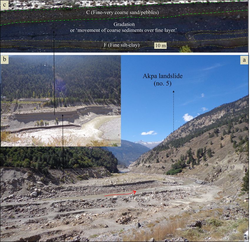
Earth Surf. Dynam., 9, 351–377, 2021 https://doi.org/10.5194/esurf-9-351-2021V. Kumar et al.: Inferring potential landslide damming using slope stability 365 Figure 8. Landslide damming indices: (a) Morphological Obstruction Index (MOI), (b) Hydro-morphological Dam Stability Index (HDSI), (c) landslides vs. MOI, and (d) landslides vs. HDSI. noted to owe their occurrence to the El Niño–Southern Oscil- nitude of less than 6.0, and only eight events are recorded in lation (ENSO), Equatorial Indian Ocean Circulation (EIOC), the range of 6.0 to 6.8 Ms (http://www.isc.ac.uk/iscbulletin/ and planetary warming (Gadgil et al., 2007; Hunt et al., search/catalogue/, last access: 2 March 2020). Out of these 2018). The orographic setting is noted to act as a main local eight events, only one event, i.e. at 6.8 Ms (19 January 1975), factor as evident from the relatively high rainfall (total pre- has been noted to have induced widespread slope failures cipitation = 1748 ± 594 mm yr−1 ) in the Kalpa region (oro- in the study area (Khattri et al., 1978). The majority of the graphic barrier) in the non-monsoon and monsoon seasons earthquake events in the study area occurred in the vicinity of from the year 2010 onwards (Fig. 11). Prediction of the po- the N–S oriented trans-tensional Kaurik–Chango fault (KCF) tential landslide damming sites in the region revealed that that accommodated the epicentre of the 19 January 1975 four (nos. 7, 14, 15, 19) out of five landslides that are pre- earthquake (Hazarika et al., 2017; http://www.isc.ac.uk/ dicted to be able to form dams belong to this orographic bar- iscbulletin/search/catalogue/, last access: 2 March 2020). rier region. Therefore, in view of the prevailing rainfall trend About 95 % of the total 1662 events had their focal depth since the year 2010, regional factors (as discussed above), within 40 km (Fig. 12b). Such a relatively low magnitude and and orographic setting, precipitation-triggered slope failure shallow seismicity in the region has been related to the Main events may be expected in the future. If such slope failure Himalayan Thrust (MHT) decollement as a response to the events occur at the predicted landslide damming sites, they relatively low convergence (∼ 14 ± 2 mm yr−1 ) of the Indian could certainly dam the river. and Eurasian plates in the region (Bilham, 2019) (Fig. 12c). The seismic pattern revealed that the region has been hit Further, the Himalaya-perpendicular Delhi–Haridwar ridge by 1662 events during the years 1940–2019, with the epi- that is under-thrusting the Eurasian plate in this region has centres located in and around the study area (Fig. 12a). been observed to be responsible for the spatially varied low However, ∼ 99.5 % of these earthquake events had a mag- seismicity in the region (Hazarika et al., 2017). Thus, though https://doi.org/10.5194/esurf-9-351-2021 Earth Surf. Dynam., 9, 351–377, 2021
366                                                    V. Kumar et al.: Inferring potential landslide damming using slope stability

Figure 9. Potential landslide damming locations: (a) Akpa_III landslide, (b) Baren Dogri landslide, (c) Pawari landslide, (d) Telangi land-
slide, and (e) Urni landslide. The dashed red arrow represents the direction of river flow. © Google Earth.

Earth Surf. Dynam., 9, 351–377, 2021                                                          https://doi.org/10.5194/esurf-9-351-2021
V. Kumar et al.: Inferring potential landslide damming using slope stability 367
Figure 10. Field signatures of the landslide damming near Akpa_III landslide. (a) Upstream view of Akpa landslide with the lacustrine
deposit at the left bank. (b) Enlarged view of the lacustrine deposit, with an arrow indicating the lacustrine sequence. (c) Alternating fine–
coarse sediments. F and C refer to fine (covered by dashed yellow lines) and coarse (covered by dashed green lines) sediment, respectively.
the study area has been subjected to frequent earthquakes, bris material with a ∼ 50 m wide run-out across the chan-
chances of earthquake-triggered landslides have been rela- nel in this narrow part of river valley (Fig. 9a), even at the
tively low in comparison to rainfall-triggered landslides and maximum value for the coefficient of friction (i.e., µ = 0.3)
associated landslide damming. For this reason, and due to the (Fig. 13a). Notably, not only the run-out extent but also
lack of reliable dynamic loads for major earthquake events, the flow height decrease when increasing the friction value
we have performed static modelling in the present study. (Fig. 13a1–a3). The maximum friction takes into account
However, we intend to perform dynamic modelling in the the shear resistance by slope material and the bed load on
near future if reliable dynamic load data become available. the river channel. However, apart from the frictional char-
acteristics of run-out path, turbulence of a debris flow also
4.4 Run-out analysis controls its dimension and hence consequences like poten-
tial damming. Therefore, different values of turbulence co-
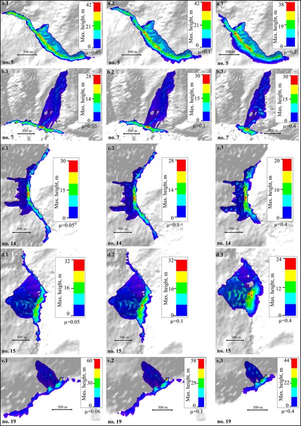
All five landslides (nos. 5, 7, 14, 15, and 19 in Fig. 9) that are efficient (ξ ) were used (Table 4). The resultant flow height
predicted to form potential landslide dams in case of slope (representing nine sets of modelled debris flows obtained us-
failure were also used for the run-out analysis to evaluate ing µ = 0.05, 0.1, and 0.3 and ξ = 100, 200, and 300 m s−2 )
expected run-out distances in the event of reactivation and attains its peak value, i.e. 39.8±4.0 m, at the base of the cen-
failure in the future. Results are as follows. tral part of landslide (Fig. 14a).
4.4.1 Akpa landslide (no. 5) 4.4.2 Baren Dogri landslide (no. 7)
Though it is difficult to ascertain the extent to which the pre- At the maximum friction value (µ = 0.4), the Baren Do-
dicted debris flow might contribute in the river blockage, it gri landslide would attain a peak value of flow height, i.e.
will certainly block the river in view of ∼ 38 m high de- ∼ 30 m, at the base of the central part of the landslide
https://doi.org/10.5194/esurf-9-351-2021 Earth Surf. Dynam., 9, 351–377, 2021368 V. Kumar et al.: Inferring potential landslide damming using slope stability Figure 11. Rainfall distribution: (a) topographic profile, (b) annual rainfall, (c) monsoonal (June–September) rainfall, and (d) non- monsoonal (October–May) rainfall. Green bars represent the years of relatively higher rainfall that resulted in flash floods, landslides, and socio-economic loss in the region. The follow references correspond to the flash flood events listed in (b). (i): http://hpenvis.nic.in/, last ac- cess: 1 March 2020; Department of Revenue, Govt. of H. P. (ii): http://hpenvis.nic.in/, last access: 1 March 2020. (iii): Kumar et al. (2019a); http://ndma.gov.in/, last access: 1 March 2020. (iv): https://sandrp.in/, last access: 1 March 2020. The numbers 1–44 refer to serial number of the landslides. (Fig. 13b). Similar to the valley configuration around the the different values of µ and ξ parameters attains a peak Akpa landslide (Sect. 4.4.1), the river valley attains a narrow value of 24.8 ± 2.7 m and decreases gradually with a run- and deep gorge setting here (Fig. 9b). The maximum value of out of ∼ 1500 m in the upstream and downstream directions debris flow height obtained using the different µ and ξ values (Fig. 14c). This landslide resulted in a relatively long run-out is 25.6±2.1 m (Fig. 14b). Flow material is also noted to attain of ∼ 1500 in the upstream and downstream directions. Apart more run-out in upstream direction of river (∼ 1100 m) than from the landslide volume affecting the run-out extent, val- in the downstream direction (∼ 800 m). This spatial variabil- ley morphology also controls the extent, as is evident from ity in the run-out length might exist due to the river channel the previous landslides. The river channel in the upstream configuration, as the river channel in the upstream direction and downstream directions from the landslide location is ob- is relatively narrow compared to the downstream direction. served to be narrow (Fig. 9c). 4.4.3 Pawari landslide (no. 14) 4.4.4 Telangi landslide (no. 15) The Pawari landslide attains maximum flow height of ∼ The Telangi landslide resulted in a peak debris flow height of 20 m at the maximum friction of the run-out path (µ = 0.4) ∼ 24 m at the maximum friction (µ = 0.4) (Fig. 13d). Upon (Fig. 13c). The resultant debris flow that is achieved using increasing the friction of run-out path, flow run-out decreased Earth Surf. Dynam., 9, 351–377, 2021 https://doi.org/10.5194/esurf-9-351-2021
V. Kumar et al.: Inferring potential landslide damming using slope stability                                                             369

Figure 12. Earthquake distribution. (a) Spatial variation of earthquakes (© Google Earth). The transparent circle represents the region within
a 100 km radius of the Satluj River (blue line). The dashed black line represents the seismic dominance around the Kaurik–Chango fault.
(b) Earthquake magnitude vs. focal depth. The dashed red region highlights the concentration of earthquakes within 40 km depth. (c) Cross
section view (based on Hazarika et al., 2017; Bilham, 2019). The dashed red circle represents the zone of strain accumulation caused by the
Indian and Eurasian plate collision (Bilham, 2019). ISC: stands for International Seismological Centre. HFT stands for Himalayan Frontal
Thrust.
https://doi.org/10.5194/esurf-9-351-2021                                                        Earth Surf. Dynam., 9, 351–377, 2021
370                                                      V. Kumar et al.: Inferring potential landslide damming using slope stability

Figure 13. Results of the run-out analysis. µ refers to the coefficient of friction.

along the river channel but increased across the river channel,             to a narrower river channel in the upstream direction than
resulting into possible damming. The debris flow after taking               in the downstream direction. The downstream side attains a
into account different values of µ and ξ parameters attains a               wider river channel due to the Main Central Thrust (MCT)
peak value of 25.0 ± 4.0 m (Fig. 14d). Similar to Baren Do-                 fault in its proximity (Fig. 1). Since the Pawari and Telangi
gri landslide (no. 7), material attained more run-out in the                landslides (nos. 14 and 15) are situated ∼ 500 m from each
upstream direction of the river (∼ 1800 m) than in the down-                other, their respective flow run-outs might mix in the river
stream direction (∼ 600 m); this difference can be attributed               channel, resulting in a disastrous cumulative effect.

Earth Surf. Dynam., 9, 351–377, 2021                                                          https://doi.org/10.5194/esurf-9-351-2021
V. Kumar et al.: Inferring potential landslide damming using slope stability                                                               371

Figure 14. Results of the run-out analysis at different values of µ and ξ . µ and ξ refer to the coefficient of friction and turbulence, respec-
tively.

4.4.5     Urni landslide (no. 19)                                         Stability Index (HDSI), were used to predict the formation of
                                                                          potential landslide dams and their subsequent stability. Rain-
The Urni landslide is predicted to attain a peak value of                 fall and earthquake regimes were also explored in the study
∼ 44 m debris flow height at the maximum friction value                   area. Finally, run-out analysis was performed for those land-
(µ = 0.4) (Fig. 13e). After considering different values of the           slides that have been observed to form the potential landslide
µ and ξ parameters, the debris flow would attain a height of              dam.
26.3 ± 1.8 m (Fig. 14e). The relatively wide river channel in                The MOI revealed that out of 44 active landslides in the
the downstream direction (Fig. 9e) results in longer run-out              Satluj valley, five of them (nos. 5, 7, 14, 15, 19) have the
in the downstream direction than in the upstream direction.               potential to form the landslide dam (Figs. 8 and 9). Upon
                                                                          evaluating the stability of such potential dam sites using the
5   Discussion                                                            HDSI, one landslide (no. 5) is predicted to attain an “uncer-
                                                                          tain” domain (5.74 < HDSI < 7.44) in terms of dam stability.
This study aimed to determine potential landslide damming                 The uncertain term implies that the resultant dam may be sta-
sites in the Satluj River valley, NW Himalaya. In order to                ble or unstable depending upon the landslide or dam volume,
achieve this objective, 44 active landslides were considered.             upstream catchment area (or water discharge), and slope gra-
First, slope stability evaluation of all the slopes at these land-        dient (Sect. 3.3). Since this landslide (no. 5) presents clear
slides sites was performed along with a parametric evalu-                 signs of having already formed a dam in the past, as indi-
ation. Then the geomorphic indices, i.e. the Morphologi-                  cated by the alternating fine–coarse layered sediment deposit
cal Obstruction Index (MOI) and Hydro-morphological Dam                   (or lake deposit) in the upstream region (Fig. 10), recurrence

https://doi.org/10.5194/esurf-9-351-2021                                                          Earth Surf. Dynam., 9, 351–377, 2021
You can also read