Fine-Scale Ocean Currents Derived From in situ Observations in Anticipation of the Upcoming SWOT Altimetric Mission
←
→
Page content transcription
If your browser does not render page correctly, please read the page content below
ORIGINAL RESEARCH
                                                                                                                                                published: 25 August 2021
                                                                                                                                          doi: 10.3389/fmars.2021.679844

                                             Fine-Scale Ocean Currents Derived
                                             From in situ Observations in
                                             Anticipation of the Upcoming SWOT
                                             Altimetric Mission
                                             Bàrbara Barceló-Llull 1*, Ananda Pascual 1*, Antonio Sánchez-Román 1 , Eugenio Cutolo 1 ,
                                             Francesco d’Ovidio 2 , Gina Fifani 2 , Enrico Ser-Giacomi 2 , Simón Ruiz 1 , Evan Mason 1 ,
                            Edited by:       Fréderic Cyr 3 , Andrea Doglioli 4 , Baptiste Mourre 5 , John T. Allen 5 , Eva Alou-Font 5 ,
                       Gilles Reverdin,      Benjamín Casas 1 , Lara Díaz-Barroso 1 , Franck Dumas 6 , Laura Gómez-Navarro 7 and
      Centre National de la Recherche        Cristian Muñoz 5
          Scientifique (CNRS), France
                                             1
                                              Institut Mediterrani d’Estudis Avançats Consejo Superior de Investigaciones Científicas - Universitat Illes Balears, Esporles,
                         Reviewed by:        Spain, 2 Sorbonne Université, CNRS, IRD, MNHN, Laboratoire d’Océanographie et du Climat : Expérimentations et
                       Daniel F. Carlson,    Approches Numériques (LOCEAN-IPSL), Paris, France, 3 Northwest Atlantic Fisheries Centre, Fisheries and Oceans Canada,
         Institute of Coastal Research,      St. John’s, NL, Canada, 4 Aix Marseille Univ., Université de Toulon, CNRS, IRD, MIO, Marseille, France, 5 Balearic Islands
   Helmholtz Centre for Materials and        Coastal Observing and Forecasting System, SOCIB, Palma, Spain, 6 Service Hydrographique et Océanographique de la
   Coastal Research (HZG), Germany           Marine, Brest, France, 7 Department of Physics, Institute for Marine and Atmospheric Research Utrecht, Utrecht University,
                   Aurélien Luigi Ponte,     Utrecht, Netherlands
  Institut Français de Recherche pour
   l’Exploitation de la Mer (IFREMER),
                                  France     After the launch of the Surface Water and Ocean Topography (SWOT) satellite planned
                *Correspondence:             for 2022, the region around the Balearic Islands (western Mediterranean Sea) will be
               Bàrbara Barceló-Llull
           b.barcelo.llull@gmail.com
                                             the target of several in situ sampling campaigns aimed at validating the first available
                    Ananda Pascual           tranche of SWOT data. In preparation for this validation, the PRE-SWOT cruise in 2018
 ananda.pascual@imedea.uib-csic.es           was conceived to explore the three-dimensional (3D) circulation at scales of 20 km
                                             that SWOT aims to resolve, included in the fine-scale range (1–100 km) as defined by
                    Specialty section:
          This article was submitted to      the altimetric community. These scales and associated variability are not captured by
                    Ocean Observation,       contemporary nadir altimeters. Temperature and salinity observations reveal a front that
                a section of the journal
           Frontiers in Marine Science       separates local Atlantic Water in the northeast from recent Atlantic Water in the southeast,
           Received: 12 March 2021
                                             and extends from the surface to ∼150 m depth with maximum geostrophic velocities of
            Accepted: 14 July 2021           the order of 0.20 m s−1 and a geostrophic Rossby number that ranges between −0.24
          Published: 25 August 2021
                                             and 0.32. This front is associated with a 3D vertical velocity field characterized by an
                                Citation:
                                             upwelling cell surrounded by two downwelling cells, one to the east and the other to
             Barceló-Llull B, Pascual A,
          Sánchez-Román A, Cutolo E,         the west. The upwelling cell is located near an area with high nitrate concentrations,
   d’Ovidio F, Fifani G, Ser-Giacomi E,      possibly indicating a recent inflow of nutrients. Meanwhile, subduction of chlorophyll-a
    Ruiz S, Mason E, Cyr F, Doglioli A,
      Mourre B, Allen JT, Alou-Font E,
                                             in the western downwelling cell is detected in glider observations. The comparison of
   Casas B, Díaz-Barroso L, Dumas F,         the altimetric geostrophic velocity with the CTD-derived geostrophic velocity, the ADCP
      Gómez-Navarro L and Muñoz C
                                             horizontal velocity, and drifter trajectories, shows that the present-day resolution of
    (2021) Fine-Scale Ocean Currents
  Derived From in situ Observations in       altimetric products precludes the representation of the currents that drive the drifter
  Anticipation of the Upcoming SWOT          displacement. The Lagrangian analysis based on these velocities demonstrates that the
                      Altimetric Mission.
             Front. Mar. Sci. 8:679844.
                                             study region has frontogenetic dynamics not detected by altimetry. Our results suggest
     doi: 10.3389/fmars.2021.679844          that the horizontal component of the flow is mainly geostrophic down to scales of 20 km

Frontiers in Marine Science | www.frontiersin.org                                    1                                            August 2021 | Volume 8 | Article 679844
Barceló-Llull et al.                                                                                             The PRE-SWOT Multi-Platform Experiment

                                             in the study region and during the period analyzed, and should therefore be resolvable
                                             by SWOT and other future satellite-borne altimeters with higher resolutions. In addition,
                                             fine-scale features have an impact on the physical and biochemical spatial variability, and
                                             multi-platform in situ sampling with a resolution similar to that expected from SWOT can
                                             capture this variability.

                                             Keywords: multi-platform experiment, in situ observations, satellite observations, SWOT, ocean currents,
                                             fine-scale, submesoscale, western Mediterranean

1. INTRODUCTION                                                                  range of fine-scales (1–100 km) as defined by the altimetric
                                                                                 community (d’Ovidio et al., 2019; Morrow et al., 2019). The study
Over the last few decades, remote sensing observations of sea                    of the oceanic features associated to these scales (such as fronts,
surface height (SSH) have greatly increased our understanding of                 meanders, eddies, and filaments) is important because they play
the global ocean large and mesoscale circulation (e.g., Chelton                  a critical role in the distribution of heat, salt, gases, carbon, and
et al., 2011; Le Traon, 2013). Altimetric observations provide                   nutrients in the global ocean (e.g., Lévy et al., 2001; Thomas,
global coverage of the ocean surface on a daily basis. The spatial               2008; Mahadevan, 2016; Klein et al., 2019). Understanding
resolution of along-track altimetric observations is however                     the 3D dynamics of these features and their impact on the
coarse, with nominal wavelengths ranging from ∼40 to ∼110                        large scale ocean circulation and climate system is one of the
km (Dufau et al., 2016). This results in a mean effective spatial                major challenges for the next decade in physical oceanography
resolution for gridded SSH maps of ∼200 km wavelength for the                    (e.g., Young and Sikora, 2003; Kwon et al., 2010; Ma et al.,
global ocean at mid-latitudes, and ∼130 km wavelength for the                    2016; Su et al., 2018; Bishop et al., 2020; Small et al., 2020).
Mediterranean Sea (Ballarotta et al., 2019). These resolutions are               Integrated approaches, combining multi-platform in situ data,
insufficient to capture the entire range of mesoscale dynamics,                  remote sensing observations and numerical modeling, constitute
especially in regional seas such as the Mediterranean, where the                 an innovative methodology for the evaluation and understanding
Rossby radius of deformation is small (∼5–15 km) and mesoscale                   of the 3D pathways associated with these structures. Some of
processes are characterized by shorter spatial scales than in other              the multi-platform experiments that have recently followed this
regions of the ocean (Chelton et al., 1998; Beuvier et al., 2012;                approach are LatMix (Shcherbina et al., 2015), AlborEx (Pascual
Escudier et al., 2016; Barceló-Llull et al., 2019; Kurkin et al., 2020).         et al., 2017; Ruiz et al., 2019), LASER (D’Asaro et al., 2020),
    The new Surface Water and Ocean Topography (SWOT)                            and CALYPSO (Mahadevan et al., 2020; Freilich and Mahadevan,
satellite mission will be launched in 2022 and it is considered                  2021; Tarry et al., 2021).
to be the next major breakthrough in satellite ocean observation                     One of the motivations to study the scales that SWOT aims
(Morrow et al., 2019). The SWOT mission aims to provide SSH                      to resolve is their importance in terms of coupled biophysical
measurements in two dimensions along a wide-swath altimeter                      processes (Lévy et al., 2018). Vertical motions associated with
track with an expected effective resolution down to wavelengths                  these features drive the vertical exchange of tracers, including
of 15–30 km. This will allow, in some regions, observation of                    nutrients and passive marine organisms, between the surface
the full range of mesoscale dynamics, i.e., scales larger than the               layers and the abyss. However, direct measurements of vertical
first Rossby radius of deformation (Fu and Ferrari, 2008; Fu and                 velocities (w) are difficult to obtain due to their small magnitudes
Ubelmann, 2014; Wang et al., 2019). During the fast-sampling                     when compared to horizontal velocities (u): O(w) ∼ (10−3 -
phase after launch, SWOT will provide observations of SSH in                     10−4 )· O(u) ∼ 10 m day−1 for the mesoscale and O(w) ∼ (10−2 )·
a 1-day-repeat orbit in specific areas of the world ocean for                    O(u) ∼ 100 m day−1 for the submesoscale (Mahadevan and
instrumental calibration and validation (d’Ovidio et al., 2019).                 Tandon, 2006; Baschek and Farmer, 2010; D’Asaro et al., 2011,
The region around the Balearic Islands (western Mediterranean                    2018). In consequence, indirect approaches have been applied
Sea) is one of the selected areas for the SWOT fast-sampling                     to calculate the vertical velocity field from observational data
phase, and will be the target of several in situ sampling campaigns              using distinct forms of the so-called omega equation or inverse
aimed at validation of SWOT measurements, and evaluation of                      methods (e.g., Hoskins et al., 1978; Viúdez et al., 1996; Pallàs-
the subsurface biophysical activity and its interaction with the                 Sanz and Viúdez, 2005; Thomas et al., 2010; Barceló-Llull et al.,
surface dynamics resolved by SWOT.                                               2017). For flows with low Rossby numbers, the quasi-geostrophic
    In preparation for these experiments, a multi-platform                       (QG) omega equation has been widely used to compute the
experiment called PRE-SWOT was conducted south of the                            vertical velocity field from observations of temperature and
Balearic Islands in 2018. The PRE-SWOT cruise objective was to                   salinity (e.g., Tintoré et al., 1991; Pollard and Regier, 1992;
collect in situ data from different observational platforms in order             Allen and Smeed, 1996; Pascual et al., 2015; Barceló-Llull et al.,
to explore the three-dimensional (3D) circulation at scales of 20                2016; Ruiz et al., 2019; Buongiorno Nardelli, 2020). Pietri et al.
km wavelength that SWOT aims to resolve (Morrow et al., 2019)                    (2021) have recently analyzed the skills and limitations of the QG
and evaluate the variability not captured by the current altimetric              omega equation in several regions of the ocean with different
constellation. The scales of 20 km wavelength are within the                     dynamics. Using a fully eddy-resolving numerical simulation

Frontiers in Marine Science | www.frontiersin.org                            2                                     August 2021 | Volume 8 | Article 679844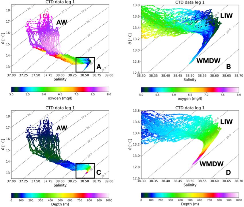
Barceló-Llull et al.                                                                                          The PRE-SWOT Multi-Platform Experiment

with a 1/16◦ horizontal resolution, they demonstrate that the                (CST-974DR), and a Biospherical irradiance radiometer. These
QG omega equation provides satisfactory results for scales larger            were attached to the rosette system of 12 oceanographic 12-
than ∼10 km.                                                                 liter Niskin bottles. Water samples were collected with the
    With the objective of improving the accuracy and reliability             rosette at different depths in some stations in order to calibrate
of altimetric observations, the European Union Copernicus                    salinity, dissolved oxygen and in vivo fluorescence (yellow stars
Programme launched the Sentinel-3A satellite mission in 2016.                in Figure 1B). Additionally, water samples for nutrients, pigment
The Sentinel-3A synthetic aperture radar altimeter (SRAL)                    signatures, and phytoplankton were taken in selected stations,
is based on the synthetic aperture radar mode (SARM)                         chosen from remote sensing ocean color maps in order to
principle proposed by Raney (1998). It has been demonstrated                 support an analysis of the main observed features (green dots in
that, compared to conventional altimetry (or low-resolution                  Figure 1B).
mode), this technique significantly reduces noise levels in the                  Leg 2 took place between 13 and 16 May 2018 and focused
measurements and increases the along-track spatial resolution                on completing four transects parallel to Sentinel-3A track 244
(Boy et al., 2017; Heslop et al., 2017; Sánchez-Román et al., 2020).         that crossed the study region on 13 May 2018 (Figure 1C). For
To focus on the analysis of (i) the fine-scale sea surface circulation       each transect the water column was sampled from the surface
over the region of study and (ii) the limitations of present-                to 500 m depth with 10 CTD casts 10 km apart; the transects
day nadir altimeters, we additionally compare observations from              were separated by 10 km. Water samples for nutrients, pigment
Sentinel-3A—together with in situ observations from an ocean                 signatures and phytoplankton determination were collected in all
glider and a ship-based hydrographic survey—with gridded                     the rosette casts of the three transects closest to Sentinel-3A track
altimetric data. This comparison complements previous studies                244 (green dots in Figure 1C). Water samples for calibration of
reported in the area by using a multi-platform approach (e.g.,               sensors were collected in one cast out of three along these three
Ruiz et al., 2009; Bouffard et al., 2010; Cotroneo et al., 2016;             transects (yellow stars in Figure 1C), while along the western
Heslop et al., 2017; Aulicino et al., 2018).                                 transect only water samples for conductivity calibration were
    The objective of this study is to compare observations from              collected (blue stars in Figure 1C). A detailed description of the
present-day altimeters with measurements from different in situ              CTD data processing and calibration can be found in the PRE-
instruments to explore the horizontal circulation at scales of               SWOT cruise report (Barceló-Llull et al., 2018). We used the
20 km that SWOT aims to resolve and evaluate the limitations                 Thermodynamic Equations of Seawater (TEOS-10) functions to
of the current altimetric constellation. We also explore the 3D              calculate potential temperature from in situ temperature, and the
QG vertical velocity field associated with the fine-scale dynamics           potential density anomaly (McDougall and Barker, 2011).
of the region of study. In addition, we analyse the relationship
between the vertical velocity field and nutrient concentrations
measured from water samples, and the chlorophyll-a signal                    2.3. ADCP
observed from an ocean glider.                                               Current velocities were continuously recorded using a hull-
                                                                             mounted 75 kHz RDI ADCP at a transit speed of ∼8 knots
2. DATA AND METHODS                                                          during the two legs of the experiment. The ADCP provided
                                                                             raw data from the surface to ∼800 m in bin sizes of 8 and 16
2.1. The PRE-SWOT Cruise                                                     m. The raw data were quality controlled, corrected for heading
The PRE-SWOT cruise was conducted aboard the R/V García                      misalignment and edited with the Common Oceanographic Data
del Cid between 5 and 17 May 2018 south of the Balearic                      Access System (CODAS, Firing et al., 1995). Further details of the
Islands (western Mediterranean Sea). Observations from in situ               ADCP data processing can be found in the PRE-SWOT cruise
platforms, including two gliders, twelve drifters, a Conductivity            report (Barceló-Llull et al., 2018).
Temperature Depth (CTD) probe attached to a rosette system,
a hull-mounted 75 kHz RDI Acoustic Doppler Current Profiler
(ADCP), and water samples taken at different depths, were                    2.4. Drifters
collected together with satellite data.                                      During Leg 1, twelve surface velocity program (SVP) drifters
                                                                             with a drogue centered at 15 m depth were deployed within the
2.2. Rosette CTD Casts and Water Samples                                     region of study. The aim was to sample frontal areas and study
The field experiment was divided into two legs. Leg 1 took place             relative dispersion by horizontal stirring at the mesoscale and
between 6 and 10 May 2018 (4.5 days) with CTD sampling over a                submesoscale. For that purpose, the drifters were arranged into
3D high-resolution regular grid in order to resolve the fine-scales          triangles with a separation between drifters of 5 km (red dots
expected from SWOT (Gómez-Navarro et al., 2020). During Leg                  and triangles in Figure 1B). Drifter deployment locations were
1 we made 63 rosette CTD casts at intervals of 10 km, resulting in           chosen based on fronts that were visible in ocean color imagery.
a regular grid of 60 × 80 km (Figure 1B). The maximum depth of               To remove the inertial signals, the drifter trajectories were filtered
most of the CTD casts was 500 m (pink dots in Figure 1B), with               using a fifth-order Butterworth low-pass filter with a cutoff of
3 casts down to 1,000 m (blue dots in Figure 1B). The rosette                1.5 times the inertial period of the area, which corresponds to
carried an SBE 911plus CTD instrument that was additionally                  19 hours (Essink et al., 2019). The zonal and meridional velocity
equipped with SeaPoint Fluorometer and Turbidity sensors, a                  components of each drifter were computed by finite differencing
SBE43 dissolved oxygen sensor, a WetLabs Transmissometer                     their trajectories.

Frontiers in Marine Science | www.frontiersin.org                        3                                      August 2021 | Volume 8 | Article 679844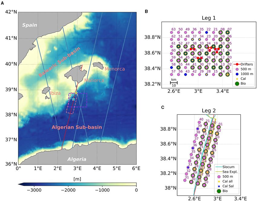
Barceló-Llull et al.                                                                                                           The PRE-SWOT Multi-Platform Experiment

  FIGURE 1 | (A) Bathymetric map of the study region. Purple and pink boxes show the regions sampled during Leg 1 and Leg 2, respectively, of the PRE-SWOT field
  experiment. Blue solid lines represent the limits of future SWOT swaths during the fast-sampling phase. Red line shows the Sentinel-3A ground-track 244 that passed
  over the Balearic Sea on 13 May 2018. Cyan and green stars represent the position of the Slocum and SeaExplorer gliders, respectively, during the satellite pass. (B)
  Leg 1 sampling strategy. (C) Leg 2 sampling strategy. Red line represents the Sentinel-3 track 244 passover on 13 May 2018. Cyan and green lines show the routes
  of the Slocum and SeaExplorer gliders, respectively, following the satellite track from 5 to 14 May 2018. In the legends: Cal and Cal all, water samples collected to
  calibrate salinity, dissolved oxygen and chl-a fluorescence; Cal Sal, water samples collected to calibrate salinity; Bio, water samples collected for nutrient, pigment
  signature, and phytoplankton determination; 500 (1,000) m, CTD casts to a maximum depth of 500 (1,000) m.

2.5. Gliders                                                                            which concentrations are derived, and with a WetLabs ECO
As part of the PRE-SWOT multi-platform experiment, two                                  FLBBCD for the measurements of chl-a fluorescence (λEx/λEm:
underwater gliders followed the Sentinel-3A track 244 (red                              470/695 nm), backscattering at 700 nm (BB700) and humic-
line in Figures 1A,C): one Slocum from the Balearic Islands                             like fluorophore fluorescence (λEx/λEm: 370/460 nm). The
Coastal Observing and Forecasting System (SOCIB) and one                                manufacturer’s calibrations were applied to all these sensors.
SeaExplorer from the Mediterranean Institute of Oceanography                            Additionally, the SeaExplorer was equipped with two MiniFluo
(MIO). Both gliders were equipped with a pumped CTD                                     sensors capable of measuring fluorescent dissolved organic
sensor (Seabird’s GPCTD). The Slocum glider was also equipped                           matter (DOM), including organic pollutants such as Polycyclic
with an Anderaa optode for the measurements of dissolved                                Aromatic Hydrocarbons (PAHs).
oxygen concentration (O2) and a WetLabs ECO FLNTU for the                                  On 3 May 2018, 2 days before the PRE-SWOT cruise started,
measurements of chlorophyll-a (chl-a) fluorescence (λEx/λEm:                            the Slocum and the SeaExplorer gliders were deployed south of
470/695 nm) and turbidity at 700 nm. The SeaExplorer                                    Mallorca. The glider mission plan involved 2 phases. In the first
was equipped with an O2 sensor (Seabird’s SBE-43F), from                                phase, the gliders transited during 2 days between the launch

Frontiers in Marine Science | www.frontiersin.org                                   4                                            August 2021 | Volume 8 | Article 679844
Barceló-Llull et al.                                                                                     The PRE-SWOT Multi-Platform Experiment

waypoint and the survey start-waypoint (38.94◦ N, 2.97◦ E); this         Figure 1A). We use the reprocessed product for the European
phase also served as a test and validation. During the second            Seas distributed by CMEMS with a spatial resolution of 7 km.
phase, that extended between 5 and 15 May 2018, the SOCIB                Cycle 31 is close in time with the glider mission described
glider followed the Sentinel-3A track 244 as closely as possible,        above: the glider return transects along the Sentinel-3A ground-
whilst the MIO glider sailed 5 km east of the satellite track, in        track were conducted between 9 and 14 May 2018, whilst the
parallel with the SOCIB glider. Over 10 days, both gliders made a        satellite overpassed the region on 13 May 2018. Thus, there is a
round-trip over their respective 100-km long tracks, and finished        temporal lag < 5 days between the first glider observations on
their missions back at the survey start-waypoint. Glider profiles        the return transects along the Sentinel-3A ground-track and the
sampled the water column from the sea surface to a maximum               satellite overpass. Note that this temporal lag is lower than the
depth of 650 m for both units and were collected at a spatial            temporal lag of 8–11 days that Aulicino et al. (2018) had between
resolution of about 8 km. Raw glider data from the SOCIB unit            observations in their inter-comparison of four SARAL-AltiKa
were processed with the SOCIB Glider Toolbox, which includes             cycles with glider transects in the same region of study. Only
a thermal lag correction (Garau et al., 2011; Troupin et al.,            data captured between 37.00◦ N and 39.05◦ N along the ground-
2015). Raw SeaExplorer data were also processed with the SOCIB           track were extracted in order to achieve close co-location with
Glider Toolbox, but at that moment no thermal lag correction             the glider measurements; this also reduces contamination of the
was available for the SeaExplorer. We used temperature and               altimetry data due to proximity to the coast (Aulicino et al., 2018).
salinity observations from the Slocum glider to calculate the            At the time of the satellite passover, the Slocum glider was located
dynamic height and compare the scales resolved by the glider             at 38.63◦ N, 2.80◦ E (cyan star in Figure 1A).
with the scales resolved by present altimetric products and CTD
observations. To evaluate the impact of vertical velocities on
the vertical distribution of tracers, we use chl-a concentrations
derived from the SeaExplorer fluorescence measurements and               2.7. Optimal Interpolation
equivalent of a mono-culture of phytoplankton Thalassiosira              Potential temperature, practical salinity, potential density
weissflogii (manufacturer’s calibration, https://www.whoi.edu/           anomaly, and dissolved oxygen concentration (hereafter
fileserver.do?id=199125&pt=2&p=207009).                                  temperature, salinity, density, and oxygen, respectively) data
                                                                         from Leg 1 were interpolated onto a regular grid with a vertical
2.6. Satellite Data                                                      resolution of 5 m and a horizontal resolution of 2 km. Processed
The choice of location for sampling of oceanic features                  ADCP velocity was vertically smoothed using a Loess filter
was guided and updated in real time by remote sensing                    with a half-power filter cutoff of 60 m and interpolated onto
imagery during the cruise. Ocean color (OC), SSH, and                    the same regular grid. Optimal interpolation was used for the
derived geostrophic currents from remote sensing were essential          horizontal interpolation (Bretherton et al., 1976). The data
components of the design of the sampling strategy. The OC data           covariance was calculated using a 2D Gaussian function with
were obtained from the NASA Ocean Color Level 1&2 Browser                semimajor and semiminor axes of Lx = Ly = 20 km (see section
(https://oceancolor.gsfc.nasa.gov). Level-2 data acquired by both        3.1.5 for a comparison with the empirical correlation calculated
the Moderate Resolution Imaging Spectroradiometer (MODIS)                from drifter and CTD observations). With this interpolation,
sensor aboard the Aqua satellite, and the Visible and Infrared           wavelengths smaller than the covariance function correlation
Imager/Radiometer Suite (VIIRS) sensor carried by the Suomi-             lengths (Lx and Ly) are filtered (Pallàs-Sanz et al., 2010). The
NPP satellite were used to design the Leg 1 CTD sampling                 mean fields are computed from a planar fit for temperature,
strategy and the drifter release location. MODIS Level-2 data            salinity, density, and oxygen, and are assumed to be constant
have a spatial resolution of 1 km, while VIIRS Level-2 data have a       for ADCP velocity (Rudnick, 1996). The uncorrelated noise
spatial resolution of 750 m.                                             for the interpolation of the ADCP velocity is assumed to be
   Before and during the cruise, SSH and derived geostrophic             18% of the signal variance; this is estimated as the ratio of
currents were obtained from the near-real-time gridded L4 multi-         noise-to-signal variance considering an instrumental error with
mission altimeter product for the Mediterranean Sea that is              a standard deviation of 0.01 m s−1 (Allen et al., 1996; Gomis
distributed by the Copernicus Marine Environment Monitoring              et al., 2001). The uncorrelated noise for the interpolation of CTD
Service (CMEMS). After the cruise ended, the reprocessed                 observations is set to 3% of the signal variance (Barceló-Llull
product had become available. Absolute Dynamic Topography                et al., 2017); this value is based on instrumental error and
(ADT) was also used to assess the oceanographic context of the           the variance of the field. Other authors have used a range of
experiment. The Mediterranean gridded Level-4 (L4) altimetric            noise-to-signal ratios from 0.01% (Ruiz et al., 2019) to 5%
products have daily time resolution and 0.125◦ × 0.125◦ grid             (Rudnick, 1996), in our case we have tested this ratio for different
resolution. ADT is computed by adding the mean dynamic                   instrumental errors and found that 3% ensures the filtering of
topography (MDT) from Rio et al. (2014) to the satellite sea level       noise due to instrumental errors. Note that the observations
anomaly (SLA) observations.                                              reconstructed through optimal interpolation are collected during
   We also used 1 Hz along-track level-3 (L3) ADT data collected         4.5 days and with this interpolation we assume that they are
by the Sentinel-3A satellite mission along the ground-track 244          quasi-synoptic, i.e., a stationary representation of the ocean at
(cycle 31). This cycle is associated with the passover of the            the scales resolved of 20 km (e.g., Rudnick, 1996; Pascual et al.,
satellite over the Algerian Basin on 13 May 2018 (red line in            2004; Barceló-Llull et al., 2017; Ruiz et al., 2019).

Frontiers in Marine Science | www.frontiersin.org                    5                                     August 2021 | Volume 8 | Article 679844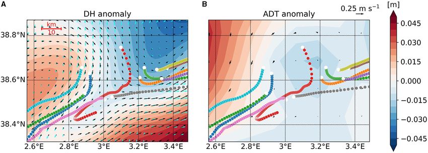
Barceló-Llull et al.                                                                                           The PRE-SWOT Multi-Platform Experiment

2.8. Dynamic Height and Geostrophic                                         (τ ) needed for initially close particles separated by an initial
Velocity Calculation                                                        distance d0 at time t0 to reach a prescribed final separation df .
Dynamic height (DH) and geostrophic velocity fields were                    The equation that defines an FSLE is the following:
computed from the optimally interpolated density data from Leg                                                      1     df

1, assuming a reference level of 1,000 m depth (1,010 dbar),                                 λ(d0 , df ; x0 , t0 ) = log                  (1)
                                                                                                                    τ     d0
the maximum depth of the CTD measurements. DH was also
calculated using the Slocum glider transect data. Temperature               An FSLE, therefore, measures the exponential rate of separation
and salinity measurements collected during the return transect              among particle trajectories. It can be computed forward or
(between 9 and 14 May 2018) were used to compute DH at 30 m                 backward in time. The forward calculation studies the dynamics
depth, as the glider subsurface inflection depth was 15 m and the           that drifters initialized nearby undergo in terms of their relative
spatial resolution of glider profiles was low in the shallower layers       distance. On the other hand, the backward separation is used
(Heslop et al., 2017). The reference level for the calculation was          to estimate regions where water masses far away in the past
set to 650 dbar (maximum depth of the glider measurements).                 are brought into contact by the circulation. The points of the
To compare glider and CTD observations from Leg 1, we also                  line along which these confluence dynamics occur all have
computed DH from the optimally interpolated density data, with              relatively high values in maps of FSLEs, and they form what
an assumed reference level of 650 dbar.                                     is called Lagrangian fronts (Prants et al., 2014) and belong to
   Leg 2 CTD data obtained along the four transects parallel                the class of Lagrangian Coherent Structures (Haller and Yuan,
to the glider tracks (Figure 1C) were used to compute DH at                 2000). Water parcels and arrays of drifters are stretched along
30 m depth. In Leg 2, CTD casts sampled the water column                    Lagrangian fronts, which act as barriers to transport. More details
down to 500 m depth, and the reference level for the inference              on Lyapunov computation and its meaning can be found in
of the DH was set to 500 dbar. The DH calculated along the                  d’Ovidio et al. (2004) and Lehahn et al. (2018).
four CTD transects was compared to that computed from the                       Backward FSLEs were computed from the numerical
Slocum glider during the return transect, also referenced to 500            trajectories in order to identify Lagrangian fronts (and hence
dbar for consistency.                                                       transport barriers) present in the velocity fields derived from
   The DH calculated from glider data is compared to the ADT                altimetry, CTD, and ADCP observations. This was done in order
obtained from both the Sentinel-3A dataset and the L4 altimetric            to test whether the trajectories of drifters released during the
gridded product. Prior to the comparison, a low-pass Loess filter           cruise were aligned along these fronts. For this application, the
(Cleveland and Devlin, 1988) with a cutoff of 30 km was applied             prescribed initial and final separation distances were optimized
to the glider, CTD and Sentinel-3A datasets in order to remove              for better visualization of the fronts with values of 1 and 20
measurement noise and small-scale variability (see e.g. Heslop              km, respectively, which are typical values used for this type of
et al., 2017). The efficiency of this approach for the comparison           application (d’Ovidio et al., 2004; Hernández-Carrasco et al.,
of DH and ADT, and the derived geostrophic velocities, has been             2011). This calculation was repeated at different depths (5, 50,
demonstrated in previous studies in the same area (Heslop et al.,           100, and 200 m) using the CTD-derived velocity fields to evaluate
2017; Aulicino et al., 2018).                                               the vertical extension of the Lagrangian fronts.
                                                                                Forward FSLEs were computed in order to compare the
                                                                            exponential rate of separation of numerical and in situ drifters.
2.9. Finite-Size Lyapunov Exponents                                         For a reliable comparison, the initial and final separations used
Horizontal advection was analyzed using Lagrangian methods,                 to compute the Lyapunov exponents forward in time from the
comparing trajectories of in situ and numerical drifters. The               velocity fields are defined as 7 and 45 km, respectively, which
trajectories of the numerical drifters were obtained by integrating         correspond to the separations of in situ drifters for the period in
the horizontal velocity fields derived from the altimetry, CTD,             which their relative separation is in an exponential regime (see
and ADCP observations with a fourth-order Runge-Kutta                       Figures 8E,F).
integrator and a time step of 3 h, assuming time varying altimetric
currents and stationary CTD-derived and ADCP velocity fields                2.10. Vertical Velocity Estimation
(d’Ovidio et al., 2013) during the integration period of 6 days.            The quasi-geostrophic (QG) vertical velocity field was calculated
The period of the numerical integration corresponds to the                  through the QG omega equation (Hoskins et al., 1978; Tintoré
time needed to reach a predefined final separation between                  et al., 1991; Buongiorno Nardelli et al., 2012; Pascual et al., 2015)
numerical drifters. Here we integrated the numerical drifters               using the optimally interpolated density field and the derived
until they were separated by 45 km, which corresponds to the                geostrophic velocity from Leg 1. The QG omega equation is
final separation between in situ drifters after the drifter distance        valid for Rossby numbers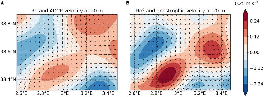
Barceló-Llull et al.                                                                                                             The PRE-SWOT Multi-Platform Experiment

  FIGURE 2 | (A–C) Ocean color images on different dates in the region of study. Data from MODIS were used on 17 April and 3 May 2018, while VIIRS data were used
  on 20 April 2018. (D–F) Absolute dynamic topography anomaly and altimetric geostrophic velocities on different dates in the region of study. For clarity, only one out of
  two current vectors are plotted. Purple and pink boxes in (C,F) delimit the regions sampled during Leg 1 and Leg 2 of the PRE-SWOT experiment, respectively.

w is the vertical velocity, ugeo is the geostrophic velocity                             for the design of the experiment. However, observations without
vector, ρ is density, ρ0 is the mean density, N 2 is the Brunt–                          cloud-coverage in the area of study were limited to some specific
                                g
Väisälä frequency (N 2 = − ρ0 ∂ρ  ∂z ), f is the Coriolis parameter,
                                                                                         days. Figures 2A–C show three examples of the best observations
considered constant and computed at the mean latitude, and                               of ocean color preceding the PRE-SWOT experiment. On 17
g is gravity. In this implementation, N 2 only depends on                                April 2018, relatively high values of chl-a of the order of 0.3 mg
depth and is estimated as the horizontal average of the Brunt–                           m−3 were observed in an elongated meander at ∼2.50◦ E, 38.00◦ N
Väisälä frequency estimated at each grid point. The Q vector                             extending to the northeast (Figure 2A). Three days after, the chl-
represents the deformation of the horizontal density gradient by                         a signal was concentrated at ∼3.20◦ E, 38.60◦ N and had values
the geostrophic velocity field. The forcing term of the QG omega                         similar to those observed in the region southeast of Mallorca
equation is on the right-hand side of (2), while on the left-hand                        and south of Menorca (Figure 2B). Two days before the cruise
side an elliptic operator is applied to the vertical velocity. The                       experiment, this signal was displaced to ∼2.90◦ E, 38.50◦ N; this
QG omega equation is solved by applying an iterative relaxation                          map was used to determine the position of the CTD casts in Leg
method with Dirichlet boundary conditions (w = 0).                                       1 and the drifter release locations (Figure 2C).
                                                                                            According to altimetric observations, the target sampling area
                                                                                         (boxes in Figure 2C) was surrounded by three oceanographic
2.11. Oceanographic Context From                                                         features: a cyclonic eddy in the Algerian basin, a cyclonic
Satellites and Sampling Region                                                           eddy south of Menorca, and an anticyclonic eddy east of Ibiza
Determination                                                                            (Figures 2D–F). The western part of the region with the chl-a
During the month before the PRE-SWOT experiment, ocean                                   signal observed at ∼2.90◦ E, 38.50◦ N on 3 May 2018 (Figure 2C)
color images provided essential information at high resolution                           was characterized by southwestern velocities of the order of

Frontiers in Marine Science | www.frontiersin.org                                    7                                             August 2021 | Volume 8 | Article 679844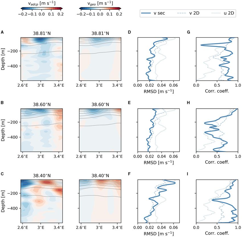
Barceló-Llull et al.                                                                                                The PRE-SWOT Multi-Platform Experiment

  FIGURE 3 | Salinity, temperature, density, and oxygen maps at (A–D) 5 and (E–H) 50 m depth from Leg 1 CTD data.

0.20 m s−1 during the month before the cruise experiment.                          signal of surface local Atlantic Water (local AW)—AW already
The persistence of the meandering flow and the presence of                         modified by a long residence in the Mediterranean. On the
an associated front visible on ocean color maps determined the                     southeastern side the front has fresher and warmer water that
region selected for the cruise experiment within the domain that                   is the signature of recent Atlantic Water (recent AW) coming
will be sampled by SWOT during the fast-sampling phase. Note                       from the Strait of Gibraltar (Barceló-Llull et al., 2019). In this
that ocean color maps (Figures 2A–C) reveal the presence of                        depth layer, density is dominated by salinity over thermal effects
filaments, eddies and fronts that are not detected in present-day                  (Figures 3C,G). At 5 m depth, dissolved oxygen is maximum
altimetric observations (Figures 2D–F). The in situ sampling is                    at the saltier side of the front, with concentration values of
then expected to provide information at high resolution which is                   7.54 mg l−1 (Figure 3D). West of 3.00◦ E the concentration is
out of reach of present-day altimeters but potentially detectable                  minimum reaching values of 7.29 mg l−1 . The dissolved oxygen
by future SWOT observations.                                                       distribution at 50 m depth does not seem related to the front
                                                                                   (Figure 3H).
3. RESULTS
                                                                                   3.1.2. Water Masses
3.1. Hydrodynamic Signature of a                                                   To analyse the different water masses residing in the region
Meandering Front                                                                   of study, temperature-salinity diagrams of all the CTD profiles
3.1.1. Hydrological Characterization                                               from Leg 1 are shown in Figure 4. A local maximum of
Maps of salinity at different depths from the Leg 1 CTD sampling                   temperature and salinity between 200 and 400 m depth reveals
reveal the presence of a meandering front in the upper layers that                 the presence of Levantine Intermediate water (LIW), and
separates saltier water at the northeastern edge of the domain                     temperature values between 12.7◦ C and 12.9◦ C are the signal
from fresher water at the southeastern edge (Figures 3A,E). The                    of Western Mediterranean Deep water (WMDW) (Pinot et al.,
signal of the front in salinity is apparent from the surface to                    2002; Balbín et al., 2012; Barceló-Llull et al., 2019). Western
∼150 m depth (not shown), having a difference of 0.8 between                       Mediterranean Intermediate water (WMIW), associated with
maximum and minimum salinity values at 5 m, the shallowest                         a relative minimum of temperature at intermediate layers,
layer of CTD observations, that decreases with depth. The map                      is not observed in the sampled region. At ∼50 m depth
of temperature at 5 m depth (Figure 3B) is characterized by a                      some profiles of saltier and colder local AW have higher
meridional distribution with warmer water at the western edge                      concentrations of oxygen than the other profiles (Figure 4A),
and colder water at the eastern edge of the sampled domain.                        which may be the signal of a local process of oxygenation. A
Below 5 m and until ∼150 m, the temperature signal resembles                       maximum of dissolved oxygen is normally formed above the deep
the front with colder water in the northeastern part of the domain                 chlorophyll maximum as a result of photosynthetic activity by
and warmer water in the southeastern part (Figure 3F). The                         phytoplankton cells. This has been observed in the northwestern
front detected between 5 and ∼150 m depth is characterized                         Mediterranean by Estrada et al. (1999), Segura-Noguera et al.
by saltier and colder water on the northeastern side that is the                   (2016), and Lefevre (2019). Between 300 and 500 m depth, higher

Frontiers in Marine Science | www.frontiersin.org                              8                                      August 2021 | Volume 8 | Article 679844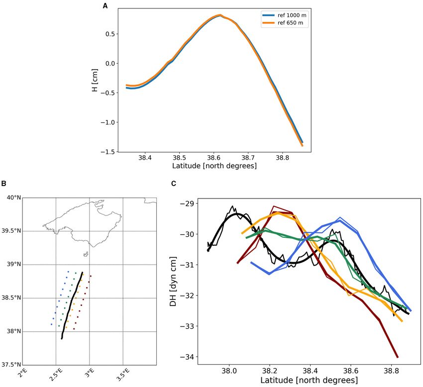
Barceló-Llull et al.                                                                                                           The PRE-SWOT Multi-Platform Experiment

  FIGURE 4 | (A–D) Temperature-salinity diagrams using data from Leg 1 CTD profiles. Color in top (bottom) plots represents the oxygen concentration (depth). The
  right column is a zoom of the left column. The presence of the following water masses is also indicated: Atlantic water (AW), Levantine Intermediate water (LIW), and
  Western Mediterranean Deep water (WMDW).

temperature and salinity values are associated with lower oxygen                        velocity (uadcp ), that includes the geostrophic and ageostrophic
concentration (Figure 4B). At depths higher than 500 m, the                             components of the flow, at 20 m depth shows a similar
oxygen concentration is almost constant.                                                circulation with differences in direction in the southeastern and
                                                                                        northwestern regions of the domain (Figure 5A, cyan arrows).
3.1.3. Geostrophic and Ageostrophic Horizontal                                          The geostrophic currents derived from altimetry (ualt ; Figure 5B)
Velocities                                                                              do not resolve the features that the ugeo and uadcp maps show.
Geostrophic velocities calculated from CTD observations (ugeo )                         This is due to the lower effective spatial resolution of altimetric
at 20 m depth reveal a meandering flow coming from the center                           gridded products in the Mediterranean (∼130 km wavelength,
north of the domain and changing its direction to the east with                         Ballarotta et al., 2019) in comparison with CTD and ADCP
a maximum speed of the order of 0.20 m s−1 (Figure 5A, black                            observations (∼20 km wavelength) that limits the representation
arrows). The southeastern part of the domain is characterized                           of the circulation in the region. Even the general circulation
by a northeastward flow reaching a maximum speed of 0.26 m                              pattern shown in the altimetric map does not correspond to
s−1 , whilst the western part shows an anticyclonic circulation                         the higher-resolution in situ velocity fields. Only in the western
with maximum speeds of the order of 0.15 m s−1 . The ADCP                               side of the domain, where a southwestward flow dominates

Frontiers in Marine Science | www.frontiersin.org                                   9                                            August 2021 | Volume 8 | Article 679844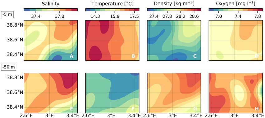
Barceló-Llull et al.                                                                                                                       The PRE-SWOT Multi-Platform Experiment

  FIGURE 5 | (A) Dynamic height (DH) anomaly at 5 m depth and geostrophic velocity vectors (in black) at 20 m depth (for consistency with ADCP velocity) calculated
  using CTD data from Leg 1. ADCP velocity vectors at 20 m depth are plotted in cyan. For clarity, only one out of two current vectors are plotted. (B) Absolute dynamic
  topography (ADT) anomaly computed from CMEMS altimetry gridded products on 3 May 2018 and derived geostrophic velocity vectors. All velocity vectors are
  plotted with the same scale. Dots show the trajectories followed by the drifters released during the PRE-SWOT experiment for the period 5–13 May; white dots are
  the release positions, and the time period between each drifter location is 2 h.

TABLE 1 | Correlation coefficients (Corr) and root mean square differences (in m s−1 , RMSD) between the zonal and meridional components of the drifter velocity and the
same components of the altimetric, ADCP and geostrophic velocities interpolated onto the drifter position (altimetric velocity was previously interpolated in time along the
drifter time axis).

                                             ualt                                                     uadcp                                                         ugeo

                             Corr                        RMSD                          Corr                         RMSD                          Corr                          RMSD

udrifters                    0.84                         0.09                          0.87                         0.06                         0.90                            0.06

                                             valt                                                     vadcp                                                         vgeo

                             Corr                        RMSD                          Corr                         RMSD                          Corr                          RMSD

vdrifters                    0.59                         0.10                          0.70                         0.05                         0.75                            0.05

The correlation coefficients are statistically significant in all cases: t tested with a confidence level of 90%, the effective degrees of freedom are calculated from the first lag of the
autocorrelation function of the drifter velocity components (7 in both cases). Note that the altimetric velocity is considered to represent the velocity at the ocean surface, the drifter
drogue was centered at 15 m depth, and the ADCP and geostrophic velocity data used for the comparison are at 20 m depth.

the circulation, ualt have similarities with ugeo and uadcp . A                                  coefficients with the three velocity fields and is maximum
visual comparison with the trajectories of the drifters released                                 with the geostrophic velocity (0.90). The meridional component
during the cruise also highlights the limitations of present-day                                 (v) has a correlation coefficient of 0.59 with the altimetric
altimetry (see drifter trajectories in Figure 5). The geostrophic                                meridional component that increases with the ADCP (0.70)
velocity calculated from CTD data and the total ADCP horizontal                                  and geostrophic (0.75) velocities. Hence, among the three
velocity show good agreement with the trajectories followed                                      datasets, the geostrophic velocity field calculated from CTD data
by the drifters, while altimetric currents cannot explain their                                  is the one showing the best agreement with the trajectories
eastward displacement.                                                                           followed by drifters. This result suggests that the strongest
    To compare quantitatively the drifter movement with ualt ,                                   component of the horizontal currents responsible for the drifter
ugeo and uadcp , we have estimated the meridional and zonal                                      displacement is geostrophic, and hence potentially resolvable
velocity components of each drifter from their trajectories                                      in higher-resolution altimetric maps like the ones that SWOT
between 5 and 12 May 2018. Table 1 shows the Pearson                                             should provide.
correlation coefficients obtained between each component of                                          Regarding the vertical distribution of horizontal velocities,
the drifter velocity and the corresponding component of                                          zonal sections of the meridional component of the ADCP
the altimetric, geostrophic and ADCP velocities. The zonal                                       velocity (vadcp ) show good correspondence with the meridional
component (u) of the drifter velocity has similar correlation                                    component of the geostrophic velocity (vgeo ) calculated from

Frontiers in Marine Science | www.frontiersin.org                                           10                                                August 2021 | Volume 8 | Article 679844
Barceló-Llull et al. The PRE-SWOT Multi-Platform Experiment FIGURE 6 | Zonal sections along (A) 38.81◦ N, (B) 38.60◦ N, and (C) 38.40◦ N of the meridional component of the optimally interpolated ADCP velocity and geostrophic velocity calculated from CTD data. Gray contours represent the potential density anomaly (the contour at the bottom is the 29.0 kg m−3 isoline and density decreases upwards with a contour interval of 0.2 kg m−3 ). Solid lines in (D–F) are the vertical profiles of the root mean square differences (RMSD) between both velocity fields along (D) 38.81◦ N, (E) 38.60◦ N, and (F) 38.40◦ N. Solid lines in (G–I) are the vertical profiles of the correlation coefficient between the corresponding velocity fields. Dashed (dotted) lines represent the vertical profiles of the RMSD (D–F) and correlation coefficient (G–I) between the meridional (zonal) velocity components considering all data in each depth layer. CTD observations (Figure 6). However, ADCP velocity has coefficient vertical profiles reveal that both fields have maximum higher magnitude and vertical variability than the geostrophic correlation in the upper ∼150 m depth, where the front is velocity field. Vertical profiles of the root mean square difference located. The correlation decreases with depth, where the vertical (RMSD) show that the differences in magnitude are higher in the variability of the ADCP velocity is more evident in comparison upper layers and decrease with depth, in correspondence with with the smoother geostrophic velocity. Dashed (dotted) lines in the decrease in magnitude of both velocities. The correlation Figure 6 represent the RMSD and correlation coefficient vertical Frontiers in Marine Science | www.frontiersin.org 11 August 2021 | Volume 8 | Article 679844
Barceló-Llull et al.                                                                                                         The PRE-SWOT Multi-Platform Experiment

  FIGURE 7 | Maps at 20 m depth of (A) Ro with ADCP velocity vectors and (B) Rog with geostrophic velocity vectors. For clarity, only one out of two current vectors
  are plotted.

profiles between the meridional (zonal) components of both                             inertial motions (Pallàs-Sanz and Viúdez, 2005; Morrow et al.,
velocity fields considering all data in each depth layer. The                          2019). The small differences observed between ADCP and CTD-
zonal components have higher RMSD and lower correlation                                derived geostrophic velocities, with maximum RMSD of the
coefficient than the meridional components of the velocities. This                     order of 0.06 m s−1 and correlation coefficients of ∼0.9 in the
translates in higher differences between the zonal velocities along                    upper layers, and the different sources of error that may introduce
meridional sections (not shown) than between the meridional                            these differences, suggest that the geostrophic component of the
velocities along the zonal transects shown in Figure 6. Hence,                         horizontal flow may dominate the local dynamics of this region
the effect of having more synoptic observations along meridional                       down to scales of 20 km.
transects than along zonal transects does not imply smaller                               The vertical relative vorticity field scaled by the planetary
differences between ADCP and geostrophic velocity fields. This                         vorticity, or Rossby number, has been estimated from ugeo (Rog )
is due to the optimal interpolation used to reconstruct the                            and from uadcp (Ro). Both fields have similar distributions and
observations, which considers all data in each depth layer.                            intensities with small differences due to the deviations observed
Note that these velocities are obtained from two independent                           between velocity fields (Figure 7). Good correspondence between
instruments and following different procedures, hence, different                       both fields is observed below 20 m depth (not shown), with
sources of error may contribute to the small differences observed                      a higher decrease with depth of the Rog magnitude due to
between both velocity fields. First, the geostrophic velocity                          the smoother ugeo field (Figure 6). Ro has values ranging from
calculated from CTD data may be underestimated as it is                                −0.26 to 0.20 and Rog between −0.24 and 0.32 in the region
calculated assuming a level of no motion of 1,000 m, while the                         of study and at the scales resolved of ∼20 km, in accordance
ADCP velocity does not have this constraint and also includes                          with a dominance of the geostrophic component of the flow
the barotropic component of the horizontal velocity, which may                         in this region for the period analyzed. Note that with higher-
increase its magnitude. In addition, from 500 to 1,000 m depth                         resolution observations we would sample smaller-scale features
the number of CTD casts is reduced and this could imply                                and the Rossby number would potentially be higher. Hence, all
an additional smoothing to the interpolated fields. Also, the                          our estimates are based on the scales we resolve of ∼20 km.
ADCP velocity field has smaller features on the southeastern and
northwestern corners of the domain (Figure 5A) that could be                           3.1.4. Finite-Size Lyapunov Exponents
due to (i) the higher resolution along meridional transects of                         The backward Lyapunov exponents computed from ualt , ugeo and
ADCP data compared to the lower resolution of CTD stations,                            uadcp are shown in Figures 8A–C. Over the Lagrangian fronts we
and (ii) potential artifacts of the optimal interpolation close to                     plot the trajectories of two drifters launched in situ on 8 May
the boundaries that may affect the estimation of the derivatives                       2018. After their release, the two drifters moved away from their
involved in the computation of ugeo . Lastly, the ADCP velocity                        deployment locations, marking an increasing separation with
has more vertical variability (Figure 6) that could be the signal of                   time (Figure 8E). The behavior of the two drifters particularly
errors coming from the instrument. In addition to the different                        underlines the classical presence of a so-called hyperbolic point
sources of error, the ADCP velocity may include ageostrophic                           in the velocity field (e.g., see Figure 3 in Lehahn et al., 2007): the
motions that are not represented in the geostrophic velocity                           drifters separate along an imaginary line, sometimes referred to as
field, such as the cyclostrophic component that could have a                           a Lagrangian front or as a Lagrangian Coherent Structure (Haller
contribution in areas of strong curvature, internal waves and                          and Yuan, 2000; Prants et al., 2014). The FSLE maps estimated

Frontiers in Marine Science | www.frontiersin.org                                 12                                           August 2021 | Volume 8 | Article 679844
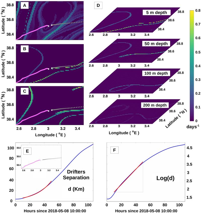
Barceló-Llull et al.                                                                                                                The PRE-SWOT Multi-Platform Experiment

  FIGURE 8 | (A–C) Backward finite-size Lyapunov exponent maps computed from (A) altimetry-, (B) CTD-, and (C) ADCP-derived velocity fields on 8 May 2018.
  These maps show the Lagrangian fronts computed from the altimetry-derived velocity at the surface, the CTD geostrophic velocity at 20 m depth, and the ADCP
  velocity at 20 m depth, respectively. Pink and gray dots represent the trajectories of two drifters released on 8 May 2018 during the PRE-SWOT experiment and
  whose release positions are indicated by the white dots. (D) Maps of the finite-size Lyapunov exponents computed from the CTD-derived velocity field at different
  depth layers (5, 50, 100, and 200 m depth). (E,F) Estimation of the exponential rate of separation for the two drifters shown in (A–C). (E) Temporal evolution of the
  distance (d) that separates both drifters. The drifters’ trajectories are displayed by the gray and pink dots in the inset plot. (F) Semi-logarithmic scale of the separation
  distance evolution with time [log(d)]. The red line represents the linear regression for the logarithmic scale corresponding to the red curve in (E) which, in turn,
  represents the exponential separation of the drifters for the period between 10 and 50 h since the release time of these two drifters.

Frontiers in Marine Science | www.frontiersin.org                                      13                                             August 2021 | Volume 8 | Article 679844
Barceló-Llull et al. The PRE-SWOT Multi-Platform Experiment
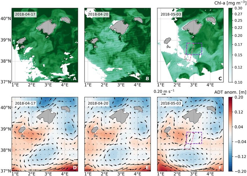
TABLE 2 | Maximum, mean, and standard deviation (STD) of the forward m day−1 . However, a sensitivity test reveals the dependence of the
finite-size Lyapunov exponents of the altimetry-, CTD-, and ADCP-derived extreme values of wQG to the correlation scales used to interpolate
Lagrangian fronts.
the original density field (Table 3). An increase of the correlation
Exponential rate of separation [days−1 ] scales from 20 to 25 km would induce a decrease on the
extreme values of wQG of about 50%. Note that applying smaller
Velocity product Maximum Mean STD
correlation scales (within the range allowed by the sampling) in
Altimetry 0.47 0.17 0.10
the optimal interpolation enables the representation of smaller-
CTD 0.72 0.45 0.17
scale variability in the interpolated fields, and this may include
ADCP 0.78 0.41 0.16
higher ageostrophic and divergent motions that would translate
to larger vertical velocities, consistent with the results from the
The initial and final separations prescribed for the computation of the finite-size Lyapunov sensitivity test. A criterion used to define the correlation scales is
exponents are chosen to match those of the in situ drifters for the period in which the
relative separation of the drifters is increasing in an exponential rate (from 10 to 50 h since
the estimation of the empirical correlation (Gomis et al., 2001;
8 May 2018 at 10:00:00). Pascual et al., 2004). Figure 10 shows the correlation of the
original density field at 100 m depth, and the correlation of the
drifter velocities (which have higher resolution than the CTD
casts). The Gaussian function that visually better resembles the
from ugeo and uadcp (Figures 8B,C) confirm this suggestion empirical correlations is likely to be the one with a characteristic
(d’Ovidio et al., 2004), while the Lagrangian fronts derived from scale of 20 km, especially for the meridional component of
ualt (Figure 8A) are inconsistent with the trajectories of the two the drifter velocity and for density. This analysis supports the
drifters, even in qualitative terms. The eastern drifter in particular correlation scales used in the optimal interpolation.
crosses an altimetry-derived Lagrangian front, which is supposed The spatial variability of nitrate and chl-a concentrations is
to behave as a transport barrier. The situation is different for consistent with the vertical velocity field calculated from CTD
the case of the CTD- and ADCP-derived Lyapunov exponents, data (Figures 9B–E). An enhancement of nitrate concentration
which display a better agreement between Lagrangian fronts and within the photic layer was detected at some stations located
drifter trajectories. Indeed, the trajectory of the two drifters is close to the upwelling cell: concentrations higher than ∼5
consistent with an expected separation along the attracting front µmol l−1 at ∼75 m are found in the 38.42◦ N and 38.50◦ N
underlined by CTD- and ADCP-derived Lyapunov exponents zonal sections at the stations located at ∼2.90◦ E and ∼3.00◦ E,
(Figures 8B,C). The Lagrangian front detected in the CTD- and also in the 38.50◦ N zonal section at the station located
derived Lyapunov exponents appears to extend vertically and at ∼3.10◦ E (Figures 9C,D). This enhanced concentration of
vanish approximately at 200 m depth (Figure 8D). nitrate within the photic layer may indicate a recent input
In order to compare the exponential rate of separation of nutrients from deeper layers induced by the upwelling cell
computed from the in situ drifter trajectories and the numerical centered at 3.05◦ E, 38.42◦ N (Figure 9A). A vertical section of
drifters, we proceeded in the following steps. We firstly identified chl-a concentration from the SeaExplorer glider return transect
a temporal window over which the relative separation between shows higher values between 100 and 180 m depth than in the
the two drifters is approximately exponential. This temporal surroundings at ∼2.85◦ E, 38.50◦ N. This may be the signal of a
window extends from 10 to 50 h since 8 May 2018 at 10:00:00 chl-a subduction related to the western downwelling cell centered
(Figures 8E,F). We then used the initial and final separations at 2.84◦ E, 38.53◦ N.
corresponding to the extrema of this temporal window (7 and
45 km, respectively) to recompute the finite-size Lyapunov
exponents from the velocity fields by simulating the trajectories 3.2. Scales Detected by the Slocum Glider
of numerical drifters. The corresponding ualt , ugeo and uadcp Along the Sentinel-3A Track
finite-size Lyapunov exponents, recomputed in this area over the 3.2.1. Glider Data vs. Altimetry Data
Lagrangian fronts, are shown in Table 2. The exponential rate Figure 11 shows the along-track ADT from the Sentinel-3A
of separation for the in situ drifters is 1.097 days−1 . Altimetry satellite mission and the DH computed from glider observations,
again has the largest mismatch with respect to the in situ drifters, together with the ADT from the gridded altimetric products
grossly underestimating their rate of separation by more than interpolated onto the glider transect. The glider DH partially
50%. CTD- and ADCP-derived exponential rates of separations captures the signature of two positive anomalies located south
are closer to the one of the in situ drifters. of the Balearic Islands at ∼38.00◦ N and ∼38.50◦ N. These two
features are located around 0.5 degrees apart in longitude, thus,
3.1.5. Vertical Velocities and Impact on Biochemical the length scale resolved by the glider data in this region has
Variability a radius of ∼13 km, the same order of magnitude of the
The horizontal distribution of the QG vertical velocity field Rossby radius of deformation in the western Mediterranean Sea
(wQG ) is similar throughout the upper 300 m depth and is (Escudier et al., 2016; Barceló-Llull et al., 2019). Not surprisingly,
characterized by an upwelling cell at the southern edge of the these two signatures are not captured by the gridded ADT
domain (3.05◦ E, 38.42◦ N) surrounded by two downwelling cells interpolated onto the glider transect (brown line in Figure 11)
at 3.28◦ E, 38.48◦ N and 2.85◦ E, 38.53◦ N (Figure 9A). At 85 m due to both its lower spatial resolution and the correlation
depth wQG has maximum values ranging between −7.7 and 7.9 length scale applied to construct the gridded product (100 km).
Frontiers in Marine Science | www.frontiersin.org 14 August 2021 | Volume 8 | Article 679844You can also read