Theoretical study of the flow in a fluid damper containing high viscosity silicone oil: effects of shear-thinning and viscoelasticity
←
→
Page content transcription
If your browser does not render page correctly, please read the page content below
Theoretical study of the flow in a fluid damper containing high viscosity silicone
                                                                    oil: effects of shear-thinning and viscoelasticity

                                                                           Alexandros Syrakosa,∗, Yannis Dimakopoulosa , John Tsamopoulosa
                                                     a
                                                         Laboratory of Fluid Mechanics and Rheology, Department of Chemical Engineering, University of Patras, 26500 Patras,
                                                                                                              Greece

                                                   Abstract
                                                   The flow inside a fluid damper where a piston reciprocates sinusoidally inside an outer casing containing
                                                   high-viscosity silicone oil is simulated using a Finite Volume method, at various excitation frequencies. The
arXiv:1802.06218v1 [physics.comp-ph] 17 Feb 2018

                                                   oil is modelled by the Carreau-Yasuda (CY) and Phan-Thien & Tanner (PTT) constitutive equations. Both
                                                   models account for shear-thinning but only the PTT model accounts for elasticity. The CY and other gener-
                                                   alised Newtonian models have been previously used in theoretical studies of fluid dampers, but the present
                                                   study is the first to perform full two-dimensional (axisymmetric) simulations employing a viscoelastic con-
                                                   stitutive equation. It is found that the CY and PTT predictions are similar when the excitation frequency
                                                   is low, but at medium and higher frequencies the CY model fails to describe important phenomena that
                                                   are predicted by the PTT model and observed in experimental studies found in the literature, such as the
                                                   hysteresis of the force-displacement and force-velocity loops. Elastic effects are quantified by applying a
                                                   decomposition of the damper force into elastic and viscous components, inspired from LAOS (Large Am-
                                                   plitude Oscillatory Shear) theory. The CY model also overestimates the damper force relative to the PTT,
                                                   because it underpredicts the flow development length inside the piston-cylinder gap. It is thus concluded
                                                   that (a) fluid elasticity must be accounted for and (b) theoretical approaches that rely on the assumption
                                                   of one-dimensional flow in the piston-cylinder gap are of limited accuracy, even if they account for fluid
                                                   viscoelasticity. The consequences of using lower-viscosity silicone oil are also briefly examined.

                                                                                 This is the accepted version of the article published in:
                                                                                Physics of Fluids 30, 030708 (2018); doi:10.1063/1.5011755

                                                   1. Introduction

                                                       Viscous dampers are devices that dissipate mechanical energy into heat through the action of viscous
                                                   stresses in a fluid; such stresses develop because the fluid is forced to flow though a constriction. A common
                                                   design involves the motion of a piston in a cylinder filled with a fluid, such that large velocity gradients
                                                   develop in the narrow gap between the piston head and the cylinder, resulting in viscous and pressure forces
                                                   that resist the piston motion. Viscous dampers are used in a range of applications, including the protection
                                                   of buildings and bridges from damage induced by seismic and wind excitations [1, 2], and the absorption of
                                                   shock and vibration energy in vehicles [3, 4] and aerospace structures [5].
                                                       A common mathematical model used to describe the behaviour of fluid dampers assumes that the
                                                   instantaneous damper force F depends only on the instantaneous piston velocity U according to

                                                                                                           F = C Un                                                        (1)

                                                   where C is the damping constant and n is an exponent usually in the range 0.3 to 2 [6]. Dampers that
                                                   conform to the above relationship are characterised as purely viscous dampers. Also, they are classified as

                                                      ∗
                                                       Corresponding author
                                                       Email addresses: syrakos@upatras.gr, alexandros.syrakos@gmail.com (Alexandros Syrakos),
                                                   dimako@chemeng.upatras.gr (Yannis Dimakopoulos), tsamo@chemeng.upatras.gr (John Tsamopoulos)

                                                   Preprint submitted to Physics of Fluids                                                                   February 20, 2018
linear if n = 1 or nonlinear if n 6= 1. Although Eq. (1) often describes well the behaviour of fluid dampers
in a range of operating conditions, dampers in many cases also exhibit a spring-like behaviour, especially at
high frequencies, where the damper force has a component that is in phase with the piston displacement. For
linear dampers, a simplifying analysis [1, 6] shows that if a sinusoidal piston displacement X = X0 sin(ωt)
is forced upon the damper and the resulting force is at a phase lag with the piston velocity then this force
can be expressed as
F = C Ẋ + K X (2)
where the dot denotes differentiation with respect to time (Ẋ ≡ dX/dt ≡ U ) and K is called the storage
stiffness. Equation (2) essentially assumes that the actual damper can be modelled as an ideal linear
purely viscous damper connected in parallel with an ideal spring. Alternatively, one can assume these two
components to be connected in series, which results in the macroscopic Maxwell model [1]:
F + λḞ = C Ẋ (3)
where λ ≡ C/K is called the relaxation time of the model. Macroscopic models of the damper behaviour
such as (1), (2) and (3) are needed for the prediction of the dynamic response to excitations of structures
that incorporate dampers. These and many more such models that have been proposed over time (see e.g.
[7–9] and references therein) are mostly phenomenological, i.e. they are not derived from first principles but
are empirical relationships. Each model incorporates a number of parameters such as C and λ whose values
have to be obtained by fitting the model to experimental data for each particular damper.
The mechanical behaviour of a fluid damper depends on several factors (damper design and dimensions,
fluid properties, operating conditions) and to obtain insight into the role of each of these one has to consider
the damper operation from first principles. Energy dissipation occurs as the mechanical excitation causes
parts of the damper to move relative to each other, forcing fluid through an orifice. Therefore the equations
governing fluid flow must be considered. The flow is in general multidimensional and time-dependent, but
in several studies simplifications have been made to make it amenable to solution by analytical means or
by simple numerical methods. The simplifications commonly made are: (a) that the only important region
is that of the orifice; (b) that the orifice is narrow and long so that the flow there can be assumed one-
dimensional; and (c) that the flow is quasi-steady, i.e. the effect of the time derivatives in the governing
equations can be neglected. These reduce the problem to planar or annular Couette-Poiseuille flow that can
be solved to obtain the wall shear stress and pressure gradient, and hence the viscous and pressure force on
the piston.
A fluid very commonly employed in dampers, especially those used in civil engineering applications,
is silicone oil (poly(dimethylsiloxane) (PDMS) [10–12]). Studies concerning silicone oil dampers include
[1, 6, 5, 13–16]. Silicone oil is a polymeric fluid whose long molecules become aligned under shear resulting
in a drop of viscosity; this property is called shear-thinning, and is more pronounced in silicone oils of
high molecular weight. Due to shear-thinning, the force with which the damper reacts to excitations is
significantly lower than what it would be if the fluid viscosity was constant. Therefore, shear-thinning must
be accounted for in theoretical studies, and a popular constitutive equation that can describe this sort of
behaviour is the Carreau-Yasuda (CY) [17] model. The CY model has been used in [16] for a theoretical study
of the flow in a silicone oil damper under the aforementioned simplifying assumptions of one-dimensional
flow that render the problem amenable to analytical solution. Two dimensional (axisymmetric) simulations
of the whole flow have also been performed, assuming silicone oil to behave as either a Newtonian [14] or a
CY fluid [18], using commercial Computational Fluid Dynamics (CFD) solvers.
Silicone oil, like most polymeric fluids, possesses another property, namely elasticity, which is a tendency
to partially recover from its deformation. The CY constitutive equation, being of generalised Newtonian
type, relates the stress tensor only to the instantaneous rate of strain tensor and hence cannot describe elastic
effects, which depend on the flow history. Constitutive equations that predict elastic behaviour are more
difficult to solve than generalised Newtonian ones and hence theoretical analyses usually assume elasticity
to be negligible and generalised Newtonian models such as CY to be sufficient. Yet, the CY model fails to
predict the stiffness aspect of the damper’s behaviour mentioned above, and it is natural to wonder whether
this stiffness is due to the elasticity of silicone oil. This has been investigated in a couple of theoretical
studies employing the one-dimensional flow simplifying assumption [19, 14] which suggest that indeed fluid
elasticity is a cause of damper stiffness, although this has been disputed in favour of fluid compressibility
2as the cause [20, 16]. A better picture would be obtained by performing simulations of the whole flow
using a viscoelastic constitutive equation, and to the best of the authors’ knowledge the present study is
the first to attempt this. A possible reason for the lack of such prior studies is that viscoelastic simulations
are much more expensive than those involving generalised Newtonian fluids such as the CY, as additional
differential equations have to be solved (one per stress component), which are unwieldy at high elasticity
(the notorious high-Weissenberg number problem – see e.g. [21]), while also much smaller time steps are
needed in order to capture the elastic phenomena (whereas if the flow is assumed generalised Newtonian, it
is also quasi-steady due to the high viscosity of typical damper fluids and one can employ large time steps
without loss of accuracy – see [22]).
In the present paper we present flow simulations in a fluid damper containing high-viscosity silicone oils,
modelled as single-mode linear Phan-Thien & Tanner [23] (PTT) viscoelastic liquids. The simulations are
performed with an in-house Finite Volume solver. The PTT constitutive equation accounts for both shear-
thinning and elasticity, and its parameters were selected so as to represent the rheological behaviour of high-
viscosity silicone oils as recorded in the literature [10–12]). The viscoelastic simulations are complemented
by simulations using the Carreau-Yasuda model which only accounts for shear-thinning but not elasticity,
so as to investigate whether this inexpensive and easy to implement alternative suffices to produce realistic
results, as has been assumed. The present results show that the PTT and CY models produce almost
identical results at low oscillation frequencies, but at medium and high frequencies the PTT model does
predict significant damper stiffness behaviour whereas the CY model does not. Furthermore, the PTT
model, contrary to the CY, predicts significant variation of the fluid velocity along the piston-cylinder gap,
i.e. that the flow in the gap is two-dimensional. This means that the theoretical approach based on the one-
dimensional viscoelastic flow assumption, employed in [19, 14], is of limited accuracy. The study concludes
with a brief investigation of flow with silicone oil of lower viscosity, to expose the main differences with the
high-viscosity case.
Before ending this introductory section, it is worth mentioning that damper stiffness is observed ex-
perimentally also in other types of fluid damper, including magnetorheological (MR) [24, 3, 20, 8, 25] and
extrusion dampers [26]. The experimental hysteresis loops obtained for these kinds of dampers are also
qualitatively very similar to the present PTT results (but not the CY results), indicating that fluid elastic-
ity is an important factor for these dampers as well. The fluids employed in MR and extrusion dampers
additionally possess a yield stress, i.e. a limiting value of stress below which they do not flow but behave as
solids; theoretical studies have thus far concentrated on the effect of yield stress, employing the Bingham
[27, 28, 25, 22] or Herschel-Bulkley [20] constitutive models to describe the viscoplasticity of these fluids, but
neglecting the elasticity. These models can explain the non-linear force-velocity relationship such as that
expressed by Eq. (1), but not the damper stiffness (the spring-like property) such as expressed by Eqs. (2)
and (3). The present results suggest that elasticity must be incorporated into these viscoplastic constitutive
equations in order to obtain more realistic predictions.
2. Problem definition and governing equations
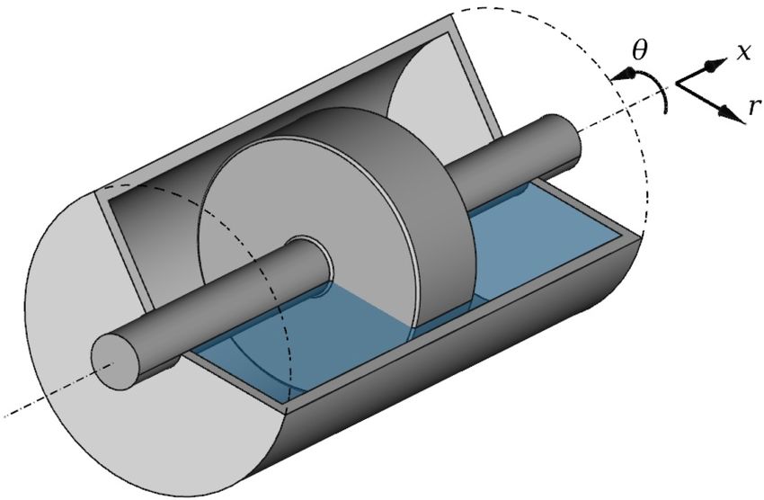
The geometry of the damper under consideration is shown in Fig. 1. It is of a simple and common
design, consisting of a cylindrical piston of radius Rp and length Lp that reciprocates in a cylinder of radius
Rc , forcing the fluid to flow through the annular gap of width h = Rc − Rp . The piston is fixed on a shaft
of radius Rs that extends on both sides of the piston so that, as the shaft and piston oscillate, the fluid
volume remains constant and compressibility effects are minimised; in fact in the present study the fluid is
assumed to be incompressible in order to isolate the effects of the fluid viscoelasticity from other possible
sources of damper stiffness such as fluid compressibility. The dimensions of the damper are listed in Table
1; they are in the range of sizes of silicone oil dampers used in experimental studies such as [14, 18]. In the
literature the relative gap width h/Rc varies from small values for low viscosity oils (e.g. 0.022 for 1 Pa s oil
in [14]) to large values for high viscosity oils (e.g. 0.412 for 630 Pa s oil in [16]), since the maximum damper
force increases by increasing the fluid viscosity but decreases by increasing the gap width. In the present
work the chosen model fluids have nominal viscosities of 100 and 500 Pa s and the relative gap width is set
to h/Rc = 0.120.
This geometry is best fitted by a system of cylindrical polar coordinates (x, r, θ) (Fig. 1a), with ex , er , eθ
denoting the unit vectors along the coordinate directions. The flow is assumed to be axisymmetric, so that
3Lc
Lp
h
Rc Rp
r
Rs x
×
(a) 3-D model (b) 2-D section
Figure 1: Layout of the damper. In (a) part of the cylinder is removed to reveal the shaft and piston. The flow is
axisymmetric and can be solved on a single plane θ = 0 (coloured in (a)).
the solution is independent of θ and the problem is reduced to two dimensions. The fluid velocity is denoted
by u, and its components are denoted by u = u · ex (axial component) and v = u · er (radial component).
The azimuthal velocity component, u · eθ , is zero. The shaft is set to reciprocate along the axial direction
such that the x−coordinate of the midpoint of the piston changes in time as
xp (t) = α cos(ωt) (4)
where x = 0 is midway along the cylinder (point marked with × in Fig. 1b), α is the amplitude of oscillation,
and ω is the angular frequency related to the frequency f by ω = 2πf . The period of oscillation is
T = 1/f = 2π/ω. For civil engineering applications the relevant frequencies are typically less than 4 Hz [1]
although short, stiff structures may have natural frequencies of the order of 10 Hz [19]; in other applications,
higher frequencies may be relevant. In the present work, simulations were performed for frequencies of f =
0.5, 2, 8 and 32 Hz, while the amplitude of oscillation was held fixed at α = 12 mm. At the start of the
simulation, at time t = 0, the fluid is assumed to be at rest. Once the shaft starts to move, after a transient
period the flow will reach a periodic state where the flow field at time t will be identical to that at time
t − T . In the present work we are interested in this periodic state, and due to viscoelastic effects this is
attained faster if the initial piston velocity is zero, hence the imposed motion (4) contains a cosine term
rather than a sine term. This means that at t = 0 the piston is located at its extreme right position. The
velocity of the shaft and piston, dxp /dt, is therefore
up (t) = −αω sin(ωt) = −Up sin(ωt) (5)
where Up = ωα is the maximum piston velocity.
The flow inside the damper is governed by the following equations that express the mass and momentum
balance of the fluid, respectively, at a microscopic (but continuum) level:
∇·u = 0 (6)
Table 1: Dimensions of the damper, in millimetres (see Fig. 1b).
Cylinder radius, Rc 25
Cylinder length, Lc 110
Piston radius, Rp 22
Piston length, Lp 20
Gap width, h = Rc − Rp 3
Shaft radius, Rs 5
4∂(ρu)
+ ∇ · (ρuu) = −∇p + ∇ · τ (7)
∂t
where t is time, u is the velocity vector, p is the pressure, ρ is the density (which is constant, set to 1000
kg/m3 ), and τ is the stress tensor. To simplify the analysis the flow will be assumed incompressible and
isothermal1 . These equations must be complemented by a constitutive equation that relates the stress
tensor to the kinematics of the flow. The simplest such equation is the Newtonian one, τ = η γ̇, where η is
the fluid viscosity and γ̇ ≡ ∇u + (∇u)T (T denoting the transpose) is the rate-of-strain tensor. However,
this does not accurately describe the behaviour of polymeric liquids for all flow conditions. Such liquids
consist of long molecular chains that interact with each other in a complex manner that typically results in
a shear-thinning behaviour, i.e. the viscosity drops as the shear rate increases. This can be seen clearly in
Fig. 2 where the symbols denote viscosity measurements at different shear rates in steady shear experiments,
reported in [10, 12], for two different silicone oils with respective zero-shear viscosities of 90 and 525 Pa s.
Steady shear experiments [32] are typically performed in capillary or rotational rheometers where a velocity
u ≡ (u1 , u2 , u3 ) = (γ̇12 x2 , 0, 0) is imposed on the fluid (as in Couette flow between parallel plates), γ̇12 being
the only non-zero component of γ̇, and the τ12 component of the stress tensor τ is measured; the viscosity
is then defined as η(γ̇12 ) ≡ τ12 /γ̇12 . A simple and popular way to construct a shear-thinning constitutive
equation is then to generalise the Newtonian one by allowing η to vary, τ = η(γ̇)γ̇ where γ̇ ≡ ( 12 γ̇ : γ̇)1/2 is
the magnitude of γ̇ and the function η(γ̇) is fitted to steady shear data such as those plotted in Fig. 2.
Figure 2: Variation of steady shear viscosity with shear rate, as measured for two different silicone oils (symbols)
and predicted by constitutive models (lines). Experimental data are from [10] () and [12] (◦). The continuous lines
correspond to the linear PTT fluids lPTT-100 (blue) and lPTT-500 (red) of Table 2. Dashed lines correspond to the
Carreau-Yasuda fluids CY-100 (blue) and CY-500 (red) of Table 2, but are nearly indistinguishable from the lPTT-100
and lPTT-500 lines. Dash-dot lines correspond to exponential PTT fluids with parameters {η = 100 Pa s, λ = 0.01 s,
= 0.25} (blue) and {η = 500 Pa s, λ = 0.06 s, = 0.025} (red).
Figure 2 shows that the viscosity of silicone oil is nearly constant up to a critical shear rate beyond
which it drops continually. A generalised Newtonian model capable of describing this kind of behaviour is
1
The temperature rise of the fluid due to viscous dissipation can be important and deserves a separate study. It is investigated
theoretically in [29, 30] and experimentally in [13]. In [13], experiments performed with a damper of much larger size than
the present model, showed that if the amplitude of oscillation is significantly greater than the piston diameter then the oil
temperature in the neighbourhood of the piston can rise by 50 or more degrees Celsius during 6 oscillation cycles (the temperature
rise is smaller farther away from the piston), which leads to a 10% drop in the maximum damper force during the same period.
A force drop is expected, because such a temperature rise would reduce the oil viscosity to half its room temperature value
[10, 31]. However, other experiments (again in [13]) with a smaller damper showed negligible effect of the temperature rise on
the force magnitude, so this issue requires further investigation.
5Table 2: Model fluids used in the simulations. In every case the density is ρ = 1000 kg/m3 .
N-100: Newtonian fluid of viscosity η = 100 Pa s
lPTT-100 Eq. (9): η0 = 100 Pa s, λ = 0.01 s, = 0.25
CY-100 Eq. (8): η0 = 100 Pa s, γ̇0 = 119 s−1 , n = 0.353, m = 1.433
lPTT-500 Eq. (9): η0 = 500 Pa s, λ = 0.06 s, = 0.25
CY-500 Eq. (8): η0 = 500 Pa s, γ̇0 = 20.7 s−1 , n = 0.346, m = 1.381
the Carreau-Yasuda model [17], with four parameters2 (η0 , γ̇0 , n, m):
m n−1
γ̇ m
η(γ̇) = η0 1 + (8)
γ̇0
At low shear rates (γ̇
γ̇0 ) the model predicts Newtonian behaviour with viscosity η = η0 while at high
shear rates (γ̇
γ̇0 ) the model predicts Power-Law behaviour η = k γ̇ n−1 with shear-thinning index n and
consistency index k = η0 /γ̇0n−1 ; the exponent m determines how rapid the transition is from Newtonian to
Power-Law behaviour as γ̇ increases. As mentioned in Section 1, this model has been used to approximate
the behaviour of damper fluids in the literature.
On the other hand, generalised Newtonian models do not account for fluid elasticity, which can affect the
behaviour of the fluid in substantial ways. A popular viscoelastic model capable of describing the rheology
of shear-thinning polymeric liquids is the Phan-Thien & Tanner (PTT) model [23, 33]; it has been used
successfully to simulate several important processes of scientific and industrial interest (e.g. [34–38]). The
simplified linear version of this model [23] can be expressed as
λ O
1 + tr(τ ) τ + λτ = η0 γ̇ (9)
η0
| {z }
Y (tr(τ ))
P
where tr(τ ) = i τii is the trace of the stress tensor, λ and η0 are the fluid relaxation time and viscosity,
respectively, and the triangle denotes the upper-convected derivative
O ∂τ
+ u · ∇τ − (∇u)T · τ + τ · ∇u
τ ≡ (10)
∂t
The PTT model (9) uses also a non-negative dimensionless parameter which is related to shear-thinning.
A feel for the physical significance of the model can be obtained by noting that for = 0, and viewing the
upper convected derivative as a form of time derivative, the PTT model is analogous to the macroscopic
Maxwell model (3) albeit applied to a microscopic fluid element3 instead of to the whole damper. In fact, for
= 0 the model (9) is called the Upper Convected Maxwell (UCM) model. For > 0 the function Y (tr(τ ))
causes shear-thinning. This can be seen in Fig. 2 where the shear-thinning behaviour of the two linear PTT
model fluids of Table 2 in steady shear flow is plotted (the solution of eq. (9) for steady shear flow can be
found in [39]; see also Appendix A).
There is another version of the PTT model commonly in use, the exponential version [33], which differs
from Eq. (9) in the definition of the function Y (tr(τ )) = exp((λ/η) tr(τ )). The behaviour of a couple of
such fluids is also plotted in Fig. 2 with dash-dot lines (see Appendix A for calculation details). It was
noticed that for viscosities around 100 Pa s the exponential model predicts excessive shear thinning whereas
2
The full Carreau-Yasuda model includes a fifth parameter, the viscosity limit η∞ as γ̇ → ∞. The experimental data for
silicone oil [10, 12] such as those plotted in Fig. 2 do not reveal a non-zero such limit; therefore, we set η∞ = 0, in which case
the Carreau-Yasuda model reduces to Eq. (8).
3
The “microscopic” fluid element is still much larger than the molecular dimensions so that the fluid can be regarded as a
continuum.
6the linear PTT model was closer to the experimentally observed behaviour of silicone oil. For viscosities
around 500 Pa s the experimentally observed shear thinning is between that predicted by the two models.
In the present work it was decided to use the linear PTT model, and in particular the fluids lPTT-100 and
lPTT-500 of Table 2. The experimental data of the 90 Pa s and 525 Pa s silicone oils plotted in Fig. 2 were
used as guides in selecting the PTT parameters, although a precise fitting to the data was not performed and
the parameters were given nice, rounded values. In particular, as shown in Appendix A, the PTT parameter
η0 is equal to the viscosity at γ̇ → 0 and values of η0 = 100 Pa s and 500 Pa s were selected. On the other
hand, as also shown in Appendix A, the data of Fig. 2 are not sufficient for obtaining realistic values for
λ and individually because the curves of all PTT fluids for which the product λ2 is the same coincide.
Therefore, the value of one of these parameters must come from another type of rheological experiment.
The PTT parameter λ is intended to represent the fluid relaxation time, i.e. the time needed for stresses in
the fluid to relax after the imposed shear rate is removed (γ̇ = 0). Longin et al. [11] provide experimental
measurements of the storage and loss moduli of a 100 Pa s silicone oil, from which they derive a discrete
spectrum of N = 10 relaxation moduli gi , i = 1, . . . , 10, and associated relaxation times λi . From these we
calculated the viscosity-averaged relaxation time as
PN
gi λ2i
λ = Pi=1
N
(11)
i=1 gi λi
which gives a value of λ = 0.01 s. Assigning this value to λ for the lPTT-100 fluid, the value = 0.25 was
then chosen in order to obtain a nice viscosity versus shear rate curve compared to the data for a 90 Pa s
silicone oil given in [10] (Fig. 2). A similar procedure was followed for the lPTT-500 fluid, using data from
[12].
Flow simulations with a viscoelastic constitutive equation such as (9) are much more expensive than
those with a generalised Newtonian constitutive equation such as (8) because in the latter the stress tensor
is given by explicit expressions whereas in the former it has to be obtained through the solution of a partial
differential equation for each relevant stress component. Thus it is tempting to assume that elasticity is not
important and treat the flow as generalised Newtonian, accounting only for shear-thinning. To investigate
how realistic such an assumption is for the present flow, we performed simulations also with the Carreau-
Yasuda CY-100 and CY-500 fluids defined in Table 2, whose parameters were chosen such that they match
the lPTT-100 and lPTT-500 fluids, respectively, in the plot of Fig. 2. This was achieved by fixing η0 to 100
(for CY-100) and 500 (for CY-500) Pa s and selecting the rest of the parameters, γ̇0 , m, n, such that they
minimise the functional
γ̇2
Z
[ln (ηCY (γ̇, γ̇0 , m, n)) − ln (ηPTT (γ̇))]2 d(ln γ̇)
γ̇1
where γ̇1 = 1 (CY-100) or 0.1 (CY-500) and γ̇2 = 105 s−1 are the lower and upper limits of the shear-rate
range of Fig. 2, ηCY is the Carreau-Yasuda viscosity function (8), and ηPTT is the steady shear viscosity
of the linear PTT fluids plotted in Fig. 2. The resulting ηCY functions are plotted in dashed lines in Fig.
2 but are not discernible because they nearly coincide with the linear PTT viscosities. A few Newtonian
simulations were also performed.
To some degree, whether inertia, shear-thinning, and elasticity of the fluid are important for this par-
ticular flow can be assessed a priori. This depends on the fluid properties, damper geometry, and operating
conditions, and is expressed in terms of dimensionless numbers. Whether shear-thinning is important or not
depends on the shear rates encountered. The highest shear rates will occur at the critical region of the gap
between the piston and cylinder, when the piston velocity is maximum, i.e. when |up | = Up = ωα (Eq. (5))
at t = T /4, 3T /4, etc. At these times, the mean fluid velocity at the gap Uf can be found from the fact
that the rate of fluid volume pushed towards one side by the piston, Up (πRp2 − πRs2 ), must equal the rate
of fluid volume crossing the gap towards the other side, Uf (πRc2 − πRp2 ), as follows from mass conservation
and incompressibility. Therefore, Uf = Up (Rp2 − Rs2 )/(Rc2 − Rp2 ). Assuming that the fluid velocity roughly
varies from Up at the piston surface to −Uf at half-way between the piston and cylinder, a characteristic
shear rate can be defined as γ̇c ≡ U/(h/2) where U = Up + Uf is the relative velocity between the fluid and
the piston. Table 3 lists the values of γ̇c for the selected frequencies; from Eq. (8) or Fig. 2 we can deduce
the viscosity that corresponds to each γ̇c , and compare it to the nominal η0 . Table 3 also lists the ratios
7Table 3: Operating conditions for which simulations were performed, and associated dimensionless numbers. The
oscillation amplitude is α = 12 mm in every case.
100 Pa s 500 Pa s
f [Hz] 0.5 2 8 32 0.5 2
Up [m/s] 0.038 0.151 0.603 2.413 0.038 0.151
U [m/s] 0.16 0.64 2.57 10.27 0.16 0.64
γ̇c [s−1 ] 107 428 1711 6845 107 428
η(γ̇c )/η0 0.759 0.399 0.178 0.078 0.315 0.137
Re 0.002 0.010 0.039 0.154 0.001 0.002
Re c 0.003 0.024 0.216 1.984 0.002 0.014
Wi 1.07 4.28 17.1 68.5 6.42 25.7
De 0.005 0.02 0.08 0.32 0.03 0.12
Sr 214 214 214 214 214 214
η(γ̇c )/η0 , and from these values it is evident that shear-thinning is expected to play a very significant role,
even at low frequencies.
To assess the importance of inertia and elasticity, it is expedient to express the governing equations in
dimensionless form. To this end, we normalise lengths by half the gap width, H ≡ h/2, time by the period
of oscillation T , velocities by U = Up + Uf , and stresses and pressure by η0 U/H. Whence substituting
x = x̃H, t = t̃T , u = ũU etc. Eqs. (7) and (9) – (10) can be expressed as
1 ∂ũ ˜ ˜ + ∇ ˜ · τ̃
Re + ∇ · (ũũ) = −∇p̃ (12)
Sr ∂ t̃
∂τ̃
˜ − (∇ũ)
˜ T · τ̃ − τ̃ · ∇ũ
˜ = γ̇˜
1 + Wi tr(τ̃ ) τ̃ + De + Wi ũ · ∇τ̃ (13)
∂ t̃
where Re ≡ ρU H/η0 is the Reynolds number, Sr ≡ T /(H/U ) is the Strouhal number, Wi ≡ λU/H is the
Weissenberg number, De ≡ λ/T (= Wi / Sr ) is the Deborah number, and the tilde (˜) denotes dimensionless
quantities, with γ̇˜ ≡ γ̇/(U/H).
The Reynolds and Strouhal numbers appear in the convection terms of the momentum equation. For
this particular problem, it follows from T = 2π/ω and U = Up + Uf = αω(1 + (Rp2 − Rs2 )/(Rc2 − Rp2 )) that
Sr = α̃ 2π(Rc2 −Rs2 )/(Rc2 −Rp2 ) where α̃ ≡ α/H is the dimensionless oscillation amplitude. Thus, the inherent
inversely proportional relationship between the velocity U and the period T removes the dependence of Sr
on f and makes it a function of only the oscillation amplitude and the damper geometry, which are held
constant in the present study. The Reynolds number is an indicator of the ratio of fluid inertia to viscous
forces, and its values for each fluid / frequency combination are listed in Table 3. This definition of Reynolds
number does not account for shear-thinning and overestimates the viscous forces, so the Table includes also
a Reynolds number based on the viscosity at the characteristic shear rate, Re c ≡ ρU H/η(γ̇c ). The values of
both Reynolds numbers can be seen to be small, making the left-hand side of the momentum equation (12)
small compared to the two terms appearing in the right-hand side. Thus the role of fluid inertia is expected
to be limited in the present flow; nevertheless, the inertia terms were retained in the equations solved and
it will be seen in Sec. 4.3 that inertia does play a minor role for this flow, at high frequencies.
The Weissenberg number is an indicator of the ratio of elastic to viscous forces, while the Deborah
number is the ratio of the fluid relaxation time to a time scale characterising the flow, which in our case is
the oscillation period T [40]. Both numbers are indicative of the importance of elastic phenomena in the
flow, and it may be seen that if they tend to zero then the constitutive equation (13) tends to the Newtonian
constitutive equation. However, the values listed in Table 3 are not small, and suggest significant elastic
effects.
8Before ending this section, one more issue must be discussed. Calculation of the damper force is of crucial
importance, and is performed by integrating the stress and pressure over the surface of the piston and the
shaft. At the points where the moving shaft meets the stationary cylindrical casing the wall velocity varies
discontinuously. If the fluid is Newtonian and the no-slip boundary condition is assumed then it can be
shown [41] that the shear stress on the shaft varies as (δx)−1 , where δx is the distance from the singularity
point. The force on the shaft is equal to the integral of the shear stress over the shaft surface, i.e. it is
proportional to the integral of (δx)−1 from δx = 0 to the length of the shaft, which is infinite. Clearly, an
infinite force is not a realistic result. In our previous work [22] this hurdle was overcome by assuming a
Navier slip boundary condition, which was shown to limit the force to finite values [42], and is a realistic
assumption according to molecular simulations studies [43, 44] even for Newtonian flows. In non-Newtonian
flows slip phenomena are much more pronounced [45–48]. To be consistent with our previous approach, in
the present study we also employed Navier slip boundary conditions, in fact on all solid walls; thus, if u and
uw are the fluid and wall velocities at the boundary then
(u − uw ) · s = β(n · τ ) · s (14)
where n is the unit vector normal to the wall and s the unit vector tangential to the wall within the plane in
which the equations are solved. The slip coefficient β is assigned here values of 5 × 10⁻⁷ m/Pa s (lPTT-100
and CY-100 fluids) and 10−6 m/Pa s (lPTT-500 and CY-500 fluids). These values are significantly lower
than those used in our previous work [22]. A feel for the effect of slip in the critical region of the gap can be
obtained as follows. Assume that the flow in that region is one-dimensional and the stress on the cylinder,
(n · τ ) · s = τrx , is typically of order η(γ̇c )U/H (Table 3) when the cylinder moves with maximum velocity.
Then from Eq. (14) it follows that
U u − uw βη(γ̇c )
u − uw = β η(γ̇c ) ⇒ =
H U H
(the product βη is called the slip length). The right-hand side has values ranging from 2.5% (f = 0.5 Hz) to
0.26% (f = 32 Hz) for the 100 Pa s fluids, and from 10.5% (f = 0.5 Hz) to 4.6% (f = 2 Hz) for the 500 Pa s
fluids. Thus the slip velocity u − uw is small, but not negligible, compared to the velocity scale U and the
flow is not much affected by the wall slip (this is confirmed by the velocity profiles shown in Fig. 18, to be
discussed in Sec. 4.4). We note that the (δx)−1 stress variation of Newtonian fluids is barely non-integrable;
a variation (δx)−a would be integrable for any a < 1 and result in finite force. Therefore, it is reasonable to
expect that for shear-thinning fluids whose viscosity tends to zero as the shear rate tends to infinity, such
as those presently employed, the force would be finite even with the no-slip boundary condition. However,
this issue was not investigated further.
3. Numerical method
The equations given in the previous Section were solved using a finite volume method, which was devel-
oped on the foundation of an existing method for generalised Newtonian and viscoplastic flows [49, 50, 22].
In the present Section the method will only be summarised, while the extensions pertaining to viscoelastic
flow will be described in detail in a separate publication.
The x − r plane was discretised by a series of block-structured grids of increasing fineness, a coarse one
of which is shown in Figs. 3a and 3b. The grid changes dynamically in time in order to follow the motion
of the piston: the cells surrounding the piston up to 2.5 mm on either side translate along with it without
deforming, while the rest of the grid cells contract or expand accordingly (Figs. 3a, 3b). Since the solution
of the set of discretised equations was accelerated using a multigrid algorithm, grids of varying fineness were
created. Solutions were obtained on the three finest grids, the sizes of which are listed in Table 4. The same
Table lists the number of cells in the radial direction between the piston and the cylinder, which are of equal
radial width. Preliminary simulations suggested that using sharp piston corners does not create additional
numerical difficulties, but to be on the safe side [51] it was decided to use rounded corners, of radius 0.75
mm, as shown in Fig. 3c. The blocks in contact with these corners were constructed using an elliptic grid
generation technique [52, 53].
Concerning the discretisation of the momentum and continuity equations, we used the same method as
in our previous work [22], which employs central differencing with least-squares gradients [54] in space and
9(a)
(b) (c)
Figure 3: (a) View of a coarse grid at a time instance when the piston is at the extreme right position. (b) View at
a time instance when the piston is at the middle position. (c) Close-up of grid 2 (Table 4) near a piston corner.
Table 4: Sizes of the grids used in the simulations.
Grid total cells cells across gap
1 16,512 24
2 66,048 48
3 264,192 96
a three time level implicit scheme in time, which are second-order accurate. A complication arises in the
viscoelastic case because the viscous forces on the cell faces are not an explicit function of the velocity but
are calculated by linear interpolation of the stresses at the cells on either side of the face, which are stored as
separate variables. This results in a lack of second derivatives of velocity in the momentum equation (7) and
leaves only the first derivatives of the convection terms, which makes the solution susceptible to spurious
velocity oscillations, in exactly the same way that the appearance of only first derivatives of pressure in the
same equation gives rise to the well-known problem of spurious pressure oscillations. In the present work,
the pressure oscillations were suppressed by using a variant, proposed in [49], of the renowned “momentum
interpolation” technique [55] while the velocity oscillations were suppressed in a similar manner, by devising
a scheme for interpolation of the stresses at cell faces that is inspired from the one proposed in [56, 57]
and re-introduces (discrete) second derivatives of velocity into the momentum equation. The details of this
interpolation scheme, which follows the philosophy of our momentum interpolation scheme [49], will be given
in a separate publication. The momentum convection terms were discretised with plain central differences;
the aforementioned stress interpolation scheme proved effective in eliminating the velocity oscillations such
that a high-resolution scheme (e.g. CUBISTA – see below) was not necessary for these terms.
The viscoelastic constitutive equations were discretised along similar lines as in [56, 58]. To reduce their
stiffness, these equations were expressed in terms of the logarithm of the conformation tensor instead of
the stress tensor itself, as suggested in [59, 21, 60]. The viscoelastic constitutive equation (9) contains no
diffusion terms, and therefore again a spurious stress oscillation issue may arise; to avoid it, its convection
terms were discretised with the CUBISTA high resolution scheme [61]. At domain boundaries, all of which
are solid walls, the pressure and stresses were linearly extrapolated from the interior. The system of non-
linear algebraic equations that arise from the finite volume discretisation was solved with an extended
SIMPLE algorithm, each iteration of which includes the solution of one linear system per component of the
log-conformation tensor. The SIMPLE solver was used as a smoother in a multigrid framework [50]. For
10one of the test cases, the lPTT-500 fluid at the f = 2 frequency, the SIMPLE / multigrid solver exhibited
convergence difficulties that were overcome by applying a vector extrapolation technique [62] where each
vector contains the estimate of all log-conformation tensor components (rr, xx, rx, and θθ) at all grid cells
after a multigrid cycle.
The code was validated against available data on viscoelastic lid-driven cavity flows, which resemble the
present flow configuration in that they are bounded all around by solid walls and the flow is induced by a
moving wall. Comparison of results obtained with our code against results presented in the literature shows
very good agreement. Indicative results concerning the location and strength of the main vortex are shown
in Table 5. The model fluids include a Newtonian solvent contribution to the stress tensor: τ = τ p + τ s
where the polymeric component τ p is given by Eq. (9) and the solvent component by τ s = ηs γ̇. Then the
flow is determined by an additional dimensionless number, the viscosity ratio B ≡ ηs /(ηs + ηp ) where ηp is
the viscosity of the polymeric component, denoted as η0 in Eq. (9).
Table 5: x̃− and ỹ− coordinates (first and second columns) of the centre of the main vortex for viscoelastic flow in
a square cavity of side H, and associated value of the streamfunction there (third column). The top wall moves in
the positive x−direction with variable velocity u(x) = 16U (x/H)2 (1 − x/H)2 (for the = 0 case), or with uniform
velocity u = U (for the = 0.25 cases); The coordinates are normalised by the cavity side H and the streamfunction
by U H. The Weissenberg and Reynolds numbers are defined as Re ≡ ρU H/(ηs + ηp ) and Wi ≡ λU/H, respectively.
= 0, Wi = 1, Re = 0, B = 0.5
Saramito [63] 0.429 0.818 -0.0619
Sousa et al. [64] 0.434 0.814 -0.0619
Present results 0.434 0.818 -0.0619
= 0.25, Wi = 4, Re = 1, B = 1/9
Dalal et al. [65] 0.429 0.812 -0.0694
Present results 0.430 0.813 -0.0693
= 0.25, Wi = 4, Re = 100, B = 1/9
Dalal et al. [65] 0.783 0.767 -0.0594
Present results 0.782 0.760 -0.0600
Each damper flow simulation had a total duration of six periods, of which the first two were calculated
on grid 1, the following two on grid 2, and the last two on grid 3 (Table 4). To ensure that the last (sixth)
period represents the periodic state, we compared force versus shaft displacement diagrams for periods 2,
4 and 6, with indicative results shown in Fig. 4. As can be seen from the figures, the force changes very
little between periods 2, 4 and 6 which suggests that the periodic state is reached quickly, and also that grid
convergence has been achieved on grid 3 (because periods 2, 4 and 6 are calculated on different grids). We
note that as viscoelasticity (Wi ) increases the force difference between different grids grows, which shows
that increasing viscoelasticity necessitates the use of finer grids to maintain a given level of accuracy. The
results suggest that the error on the finest grid is in each case less than 1 %. The force calculated on grid 2
for the lPTT-100 fluid at f = 32 Hz (Fig. 4f) has a component that oscillates in time (which is responsible
for the relatively large zero-displacement force difference of 2.63% between grids 2 and 3) but this vanishes
on the finest grid.
The time step used in the simulations was ∆t = T /4000 for the CY and Newtonian fluids and ∆t =
T /8000 for the l-PTT fluids. Since the Reynolds numbers are small, the inertial terms in the momentum
Eq. (12), which include the temporal term, are not very significant and thus for the Newtonian and CY
simulations the flow is quasi-steady [22] (or nearly so) and the choice of time step is not crucial (the chosen
∆t = T /4000 is most probably unnecessarily small). On the other hand, for the viscoelastic simulations a
temporal term appears also in the constitutive Eq. (13) which, according to the values of Wi and De listed in
Table 3, may be significant; hence the small chosen time step ∆t = T /8000 for the viscoelastic simulations.
11(a) N-100, 32 Hz (0.41%, 0.08%) (b) CY-100, 0.5 Hz (0.59%, 0.14%) (c) CY-100, 32 Hz (0.90%, 0.23%)
(d) lPTT-100, 0.5 Hz (0.72%, 0.14%) (e) lPTT-100, 8 Hz (2.35%, 0.81%) (f ) lPTT-100, 32 Hz (1.36%, -2.63%)
(g) CY-500, 2 Hz (0.81%, 0.20%) (h) lPTT-500, 0.5 Hz (0.67%, -0.03%) (i) lPTT-500, 2 Hz (1.95%, -0.01%)
Figure 4: Diagrams of the force Ff l , Eq. (17), versus displacement of the piston midpoint compared to the x = 0
position, for various fluids and frequencies. Dashed lines: period 2, calculated on grid 1; dash-dot lines: period 4,
calculated on grid 2; continuous lines: period 6, calculated on grid 3. The numbers in parentheses are the percentage
difference in force at zero displacement between grid 3 and either grid 1 (first number) or grid 2 (second number).
The loops are traversed in the anticlockwise sense as time progresses.
This is 20 times smaller than that used in our previous study [22], and was found to offer adequate accuracy
by tests where the time steps used on the coarse grids 2 and 1 were, respectively, two (∆t = T /4000) and
four (∆t = T /2000) times larger than this value, which was used on grid 3. For example, this procedure
for the lPTT-100, f = 8 Hz case yielded force differences at zero displacement of 1.85% and 0.68% between
grids 3 and 1, and 3 and 2, respectively. These differences are even smaller than those reported in Fig. 4e,
which suggests that the spatial and temporal discretisation contributions to the discretisation error are of
opposite sign. The present choice of time step, which is coupled to the oscillation period, leads to variable
resolutions of the relaxation time depending on the oscillation frequency, namely to ratios λ/∆t of 40, 160,
640 and 2560 at f = 0.5, 2, 8 and 32 Hz, respectively, for the lPTT-100 fluid and of 240 and 960 at f
= 0.5 and 2 Hz, respectively, for the lPTT-500 fluid. At low frequencies this ratio is small, but the Wi
and De numbers are small as well (Table 3) and the importance of viscoelasticity diminishes, as the results
of Sec. 4 will confirm, so that a high resolution of the viscoelastic phenomena is not necessary in order to
12accurately simulate the flow. Finally, we note that the Courant-Friedrichs-Lewy number (CFL) on the finest
grid can be approximated as U ∆t/(h/96) where h/96 is the grid spacing across the gap, which gives CFL
values of 2.56 and 1.28 for the CY and l-PTT fluids, respectively (independent of the frequency f ). The
CFL number is used in explicit temporal discretisation schemes to control their stability; while the present
method is implicit and a CFL < 1 is not a prerequisite for stability, usually a CFL number smaller than
unity indicates adequate temporal resolution in relation to the spatial resolution. In [66], where the same
temporal discretisation scheme was used, good accuracy was reported with CFL numbers as high as 3–6.
4. Results
In an experimental study, the damper under investigation would be subjected to a predetermined dis-
placement history, and the required force that causes this displacement would be recorded using a load cell.
This applied force, Fap , causes the acceleration of the shaft-piston assemblage, and is counteracted by the
force Ff l exerted by the fluid on the shaft-piston and by the friction force Ff r at the damper bearings and
seals. Therefore, Newton’s second law can be expressed as
Fap + Ff l + Ff r = Mp ap (15)
where Mp is the mass of the shaft-piston assemblage and ap is its acceleration. The latter is obtained by
differentiating Eq. (5):
ap (t) = −αω 2 cos(ωt) = −Ap cos(ωt) (16)
where Ap = αω 2 is the maximum acceleration, occurring when the piston reaches its extreme positions.
The present numerical simulations allow prediction of the reaction force exerted by the fluid on the
piston and shaft, by integrating the stress and pressure over the piston surface and on the part of the shaft’s
surface that is immersed in the fluid:
ZZ
Ff l = −pn + n · τ · ex ds (17)
S
where S is the shaft-piston surface, ds is an infinitesimal element of that surface, and n is the unit vector
normal to that surface at each point, directed towards the fluid. It is mostly on this force that the present
study focuses. If the friction force Ff r and the piston inertia term Mp ap are assumed negligible, then Eq.
(15) reduces to
Fap ≈ −Ff l (18)
Therefore, the plots of Ff l presented in this study, such as in Fig. 4, resemble mirror images of experimentally
derived plots of Fap provided in the literature. However, in Section 4.5 plots of Fap itself will also be
presented, derived from Eq. (15) with the shaft inertia included but Ff r neglected.
Customarily, the damper behaviour is explored through the examination of plots of force versus piston
displacement and piston velocity, which are easily obtainable in experimental studies. The present study
includes such plots but is not restricted to these. One of the advantages of numerical simulation is that it
provides estimates of all the flow variables at every point in the domain and at every time instance, thus pro-
viding a complete picture of the flow. This is exploited in order to go beyond the force-displacement/velocity
plots and obtain additional insight. Since we are interested in the periodic state, the plots presented in this
study correspond to the sixth oscillation period simulated (t ∈ [5T, 6T ]), unless otherwise stated, in order
to avoid any initial transient phenomena (although it was noticed that the periodic state is attained fairly
quickly, with transient phenomena not persisting beyond the first period).
The area enclosed by the loops of force-displacement plots is equal to the energy absorbed by the damper
in a single cycle and converted into heat by viscous action in the fluid4 . A look at Fig. 4 shows that the
4
The instantaneous energy balance for the damper fluid includes the rate of work of the force Ff l , the rate of viscous
dissipation of energy into heat, and the rate of change of energy stored in the fluid in the form of elastic energy. However,
considering a full period of oscillation, if the flow has reached the periodic state, the stored elastic energy at time t is exactly
equal to that at time t + T . Therefore, the work of Ff l during a complete cycle is equal to the amount of energy dissipated to
heat by viscous action during the same period.
13elliptical shape of the Newtonian loop 4a is distorted towards a rectangular shape when the fluid is non-
Newtonian, stretched in a direction that forms either a positive (counterclockwise) angle, for CY fluids (e.g.
Fig. 4c), or a negative (clockwise) angle, for PTT fluids (e.g. Fig. 4i), compared to the horizontal axis. The
non-Newtonian characteristics become more prominent as the frequency and/or zero-shear viscosity (η0 )
increase. In force-displacement diagrams, this tilting of the loop at an oblique angle is a definite sign of
hysteresis, i.e. of dependence of the current state of the flow on its history.
When the Reynolds number in Eq. (12), and, for PTT fluids, the Wi and De numbers in Eq. (13),
are very small then the corresponding terms become negligible and the governing equations become elliptic
and quasi-steady state, so that the flow is not affected by its own history but is determined solely by the
instantaneous boundary conditions. In this case, symmetry between two instantaneous damper states, such
as any pair of the states (a), (b) and (c) depicted in Fig. 5, results in identical force magnitudes. Such
is the flow of the N-100 fluid even at the highest frequency of 32 Hz (Fig. 4a) because of the very large
viscosity of the fluid. In Fig. 4a the three states (a), (b) and (c) are marked (the displacement d of Fig. 5
is arbitrarily set equal to 5 mm in Fig. 4) and it can be seen that |Ff l (a)| = |Ff l (b)| = |Ff l (c)|. The N-100
loop is symmetric with respect to both the force = 0 and displacement = 0 axes.
On the other hand, for the CY and PTT fluids as the frequency increases the transient terms in Eqs.
(12) and (13) become more important and the flow history comes into play. Now, although damper states
(a) and (b) are symmetric, they have different histories and therefore |Ff l (a)| =6 |Ff l (b)| in both Fig. 4c and
Fig. 4i. However, states (a) and (c) are not only symmetric, but the histories of the flows leading up to
these states are also symmetric; therefore, |Ff l (a)| = |Ff l (c)|. Half a period suffices to describe the whole
loop (the flow fields at times t and t + T /2 are symmetric).
It is customary to also plot the force versus the piston velocity, as in Fig. 6. We shall use the normalised
velocity up /Up (Eq. (5)) for such plots, which allows to plot the loops of different frequencies on the same
diagram (the maximum piston velocities Up for each frequency are listed in Table 3). The effects of the
non-Newtonian character of the fluids are even more pronounced on force-velocity plots, especially at higher
frequencies (Fig. 6b) whereas at low frequencies the behaviour deviates mildly from the Newtonian one
(Fig. 6a). In force-velocity plots hysteresis is manifest in the plot having the form of a loop rather than of
a single curve. This means that, by drawing a vertical line on the graph, for a given piston velocity there
are two different values of force: one value is exhibited when the piston is accelerating, and a different value
when it is decelerating. This can be observed in Fig. 6b where Ff l (b) 6= Ff l (c) for both the CY and PTT
fluids, whereas Ff l (b) = Ff l (c) for the Newtonian fluid (the states (a), (b), (c) have been arbitrarily set to
correspond to a normalised velocity of ±0.3).
The force-displacement and force-velocity plots are very reminiscent of the Lissajous-Bowditch plots
obtained in Large Amplitude Oscillatory Shear (LAOS) experiments [67], i.e. plots of shear stress versus
strain or rate-of-strain, respectively, which are used for the characterisation of soft materials and complex
fluids. A brief description of LAOS is given in Appendix B. This similarity allows us to borrow some tools
from LAOS theory in the following sections. However, it must be noted that there are also significant
differences between LAOS and the present flow: whereas in LAOS all the material undergoes the same
deformation simultaneously in a Couette-type flow, the damper flow is two-dimensional and mostly pressure
driven, with the stress and deformation rate varying along both the gap length and width, while each fluid
particle remains in the critical gap region for only a limited amount of time during each period, provided
that the oscillation amplitude is not very small.
The precise shapes of the force-displacement and force-velocity plots will be examined in greater detail
in the sections that follow, but first a general description of the flow field inside the damper will be given.
4.1. General description of the flow field
Before examining the force Ff l it is worthwhile to examine some snapshots of the whole flow field in Fig.
7. All snapshots correspond to a time instance when the piston moves towards the right with maximum
velocity. The general picture that these snapshots present is that the rightward piston motion forces oil to
flow from the right damper compartment to the left compartment through the narrow annular gap, which
gives rise to a sharp pressure gradient along the gap length in order to overcome the stresses that resist this
fluid motion. The resulting large pressure difference between the left and right sides of the piston causes
a pressure force that opposes its motion. The latter is also opposed by the stresses in the gap region, but
14(a) piston approaching the extreme right
(b) piston leaving the extreme right
(c) piston approaching the extreme left
Figure 5: The damper at three different “symmetric” time instances: At (a) the piston is displaced towards the
right and is moving towards the right. Later, at (b), the piston has returned to the same position (xp (b) = xp (a))
but is moving towards the left (up (b) = −up (a)). Later still, at (c), the piston has moved to the opposite side
(xp (c) = −xp (b)) and is moving towards the left (up (c) = up (b)). The directions of the inertial and elastic components
of the fluid force on the piston and shaft are shown in each case.
the pressure contribution to the total force Ff l is much larger for this damper configuration: as shown in
Fig. 8, the pressure force is nearly ten times larger than the force due to shear stresses. Figure 8 also shows
that Ff l arises mostly on the piston surface, while the contribution of the shaft surface to the total force is
negligible.
The instantaneous streamlines shown in Fig. 7 are drawn equispaced along the vertical piston walls in
the r-direction. The flow rate between any pair of streamlines can be calculated from the piston velocity and
the area between the points where these streamlines touch the vertical piston walls. Because the domain is
axisymmetric, this area, and therefore also the flow rate, between a pair of successive streamlines that are
close to the shaft (small r coordinate) is smaller than that between a pair of successive streamlines that lie
closer to the outer cylinder (large r coordinate). Therefore, it is evident from all snapshots of Fig. 7 that
the flow is mostly restricted to the immediate neighbourhood of the piston. Fluid that gets pushed out of
the way in front of the piston quickly rises, passes through the gap, and travels to the region immediately
behind the piston. Fluid that is located farther away remains relatively at rest.
In Fig. 7, the left column of snapshots corresponds to the Carreau-Yasuda fluids, while the right column
contains the corresponding snapshots predicted by the l-PTT fluids. The Carreau-Yasuda model predicts
a smooth, symmetric flow field in every case examined. This is due to the fact that the inertial character
of this flow is weak; it is not hard to show that for a symmetric domain, such as the present one when the
15You can also read