Random forests for real time 3D face analysis
←
→
Page content transcription
If your browser does not render page correctly, please read the page content below
myjournal manuscript No.
(will be inserted by the editor)

Random forests for real time 3D face analysis
Gabriele Fanelli · Matthias Dantone · Juergen Gall · Andrea Fossati ·
Luc Van Gool

Received: date / Accepted: date

Abstract We present a random forest-based frame-              1 Introduction
work for real time head pose estimation from depth
images and extend it to localize a set of facial features     Despite recent advances, people still interact with ma-
in 3D. Our algorithm takes a voting approach, where           chines through devices like keyboards and mice, which
each patch extracted from the depth image can directly        are not part of natural human-human communication.
cast a vote for the head pose or each of the facial fea-      As people interact by means of many channels, includ-
tures. Our system proves capable of handling large ro-        ing body posture and facial expressions, an important
tations, partial occlusions, and the noisy depth data         step towards more natural interfaces is the visual analy-
acquired using commercial sensors. Moreover, the algo-        sis of the user’s movements by the machine. Besides the
rithm works on each frame independently and achieves          interpretation of full body movements, as done by sys-
real time performance without resorting to parallel com-      tems like the Kinect for gaming, new interfaces would
putations on a GPU. We present extensive experiments          highly benefit from automatic analysis of facial move-
on publicly available, challenging datasets and present       ments, as addressed in this paper.
a new annotated head pose database recorded using a               Recent work has mainly focused on the analysis of
Microsoft Kinect.                                             standard images or videos; see the survey of [47] for an
                                                              overview of head pose estimation from video. The use
Keywords Random forests · Head pose estimation ·              of 2D imagery is very challenging though, not least be-
3D facial features detection · Real time                      cause of the lack of texture in some facial regions. On
                                                              the other hand, depth-sensing devices have recently be-
                                                              come affordable (e.g., Microsoft Kinect or Asus Xtion)
Gabriele Fanelli · Matthias Dantone · Juergen Gall · Andrea   and in some cases also accurate (e.g., [66]).
Fossati · Luc Van Gool
Computer Vision Laboratory, ETH Zurich,                           The newly available depth cue is key for solving
Sternwartstrasse 7, 8092 Zurich, Switzerland                  many of the problems inherent to 2D video data. Yet,
E-mail: fanelli@vision.ee.ethz.ch                             3D imagery has mainly been leveraged for face track-
Matthias Dantone                                              ing [6, 11, 67, 65], often leaving open issues of drift and
E-mail: dantone@vision.ee.ethz.ch                             (re-)initialization. Tracking-by-detection, on the other
Juergen Gall                                                  hand, detects the face or its features in each frame,
Perceiving Systems Department, Max Planck Institute for In-   thereby providing increased robustness.
telligent Systems,
Spemannstrasse 41, 72076 Tübingen, Germany
                                                                  A typical approach to 3D head pose estimation in-
E-mail: juergen.gall@tue.mpg.de                               volves localizing a specific facial feature point (e.g., one
Andrea Fossati
                                                              not affected by facial deformations like the nose) and
E-mail: fossati@vision.ee.ethz.ch                             determining the head orientation (e.g., as Euler angles).
Luc Van Gool
                                                              When 3D data is used, most methods rely on geometry
Department of Electrical Engineering/IBBT, K.U. Leuven,       to localize prominent facial points like the nose tip [39,
Kasteelpark Arenberg 10, 3001 Heverlee, Belgium               12, 60, 10, 9] and thus becoming sensitive to its occlu-
E-mail: luc.vangool@esat.kuleuven.be                          sion. Moreover, the available algorithms are either not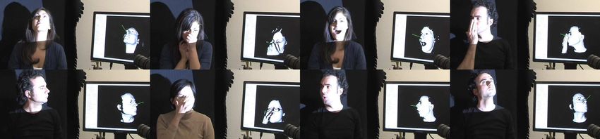
2                                                                                                 Gabriele Fanelli et al.

real time, rely on some assumption for initialization like   2 Related work
starting with a frontal pose, or cannot handle large ro-
tations.                                                     After a brief overview of the random forest literature,
     We introduce a voting framework where patches ex-       we present an analysis of related works on head pose
tracted from the whole depth image can contribute to         estimation and facial features localization.
the estimation task. As in the Implicit Shape Model [36],
the intuition is that patches belonging to different parts
of the image contain valuable information on global          2.1 Random Forests
properties of the object which generated it, like pose.
                                                             Random forests [7] have become a popular method in
Since all patches can vote for the localization of a spe-
                                                             computer vision [28, 29, 57, 30] given their capability to
cific point of the object, it can be detected even when
                                                             handle large training datasets, their high generalization
that particular point is occluded.
                                                             power and speed, and the relative ease of implementa-
     We propose to use random regression forests for
                                                             tion. Recent works showed the power of random forests
real time head pose estimation and facial feature lo-
                                                             in mapping image features to votes in a generalized
calization from depth images. Random forests [7] (RFs)
                                                             Hough space [28] or, in a regression framework, to real-
have been successful in semantic segmentation [58], key-
                                                             valued functions [19]. In the context of real time pose
point recognition [37], object detection [28, 29], action
                                                             estimation, multi-class random forests have been pro-
recognition [70, 29], and real time human pose estima-
                                                             posed for the real time determination of head pose from
tion [57, 30]. They are well suited for time-critical ap-
                                                             2D video data [32]. In [57], random forests have been
plications, being very fast at both train and test time,
                                                             used for real time body pose estimation from depth
lend themselves to parallelization [56], and are inher-
                                                             data. Each input depth pixel is first assigned to a spe-
ently multi-class. The proposed method does not rely
                                                             cific body part, using a classification forest trained on
on specific hardware and can easily trade-off accuracy
                                                             a very large synthetic dataset. After this step, the lo-
for speed. We estimate the desired, continuous param-
                                                             cation of the body joints is inferred through a local
eters directly from the depth data, through a learnt
                                                             mode-finding approach based on mean shift. In [30], it
mapping from depth to parameter values. Our system
                                                             has been shown that the body pose can be more effi-
works in real time, without manual initialization. In our
                                                             ciently estimated by using regression instead of classi-
experiments, we show that it also works for unseen faces
                                                             fication forests. Inspired by the works [28, 19], we have
and that it can handle large pose changes, variations in
                                                             shown that regression forests can be used for real time
facial hair, and partial occlusions due to glasses, hands,
                                                             head pose estimation from depth data [25, 26].
or missing parts in the 3D reconstruction. It does not
                                                                  A detailed introduction to decision forests and their
rely on specific features like the nose tip.
                                                             applications in computer vision can be found in [18].
     Random forests show their power when using large
datasets, on which they can be trained efficiently. Be-
cause the accuracy of a regressor depends on the amount      2.2 Head pose estimation
of annotated training data, the acquisition and label-
ing of a training set are key issues. Depending on the       With application ranging from image normalization for
expected scenario, we either synthetically generate an-      recognition to driver drowsiness detection, automatic
notated depth images by rendering a face model under-        head pose estimation is an important problem. Several
going large rotations, or record real sequences using a      approaches have been proposed in the literature [47];
consumer depth sensor, automatically annotating them         before introducing 3D approaches, which are more rele-
using state-of-the-art tracking methods.                     vant for this paper, we present a brief overview of works
     A preliminary version of this work was published        that take 2D images as input. Methods based on 2D
in [25], where we introduced the use of random regres-       images can be subdivided into appearance-based and
sion forests for real time head pose estimation from high    feature-based classes, depending on whether they ana-
quality range scans. In [26], we extended the forest to      lyze the face as a whole or instead rely on the localiza-
cope with depth images where the whole body can be           tion of some specific facial features.
visible, i.e., discriminating depth patches that belong to       2D Appearance-based methods. These meth-
a head and only using those to predict the pose, jointly     ods usually discretize the head pose space and learn sep-
solving the classification and regression problems in-       arate detectors for subsets of poses [33]. Chen et al. [13]
volved. In this work, we provide a thorough experimen-       and Balasubramanian et al. [2] present head pose esti-
tal evaluation and extend the random forest to localize      mation systems with a specific focus on the mapping
several facial landmarks on the range scans.                 from the high-dimensional space of facial appearance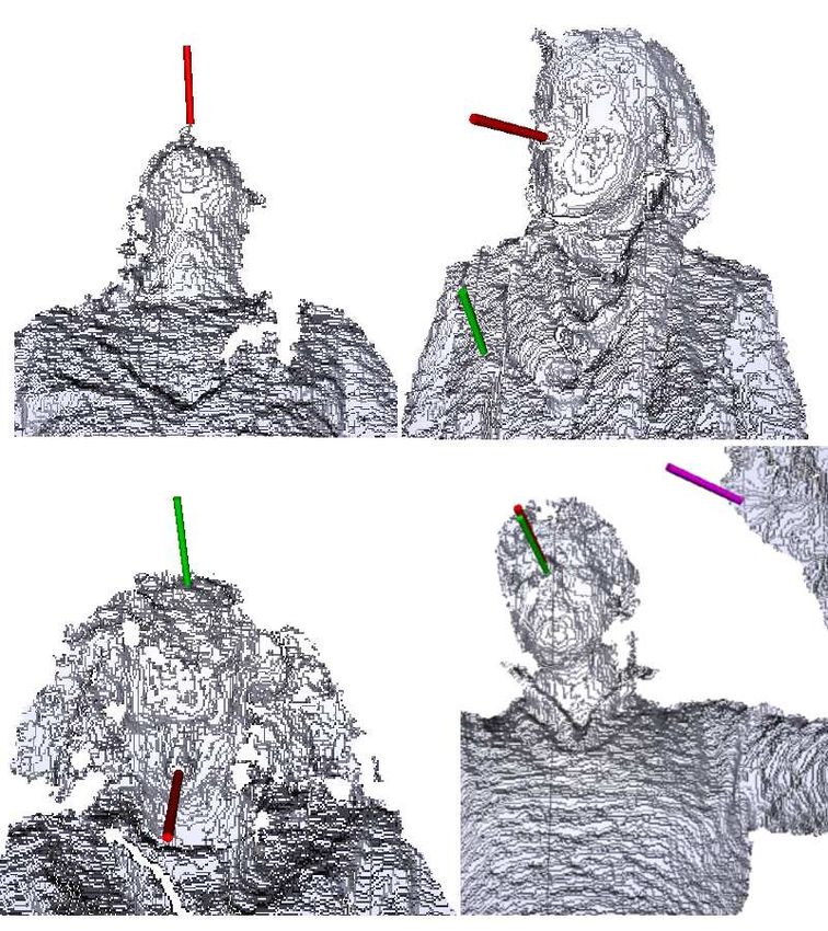
Random forests for real time 3D face analysis                                                                          3

to the lower-dimensional manifold of head poses. The          the low reported average errors are only calculated on
latter paper considers face images with varying poses         faces of subjects that belong to the training set. Still in
as lying on a smooth low-dimensional manifold in a            a tracking framework, Morency et al. [44] use instead a
high-dimensional feature space. The proposed Biased           intensity and depth input image to build a prior model
Manifold Embedding uses the pose angle information            of the face using 3D view-based eigenspaces. Then, they
of the face images to compute a biased neighborhood           use this model to compute the absolute difference in
of each point in the feature space, prior to determin-        pose for each new frame. The pose range is limited and
ing the low-dimensional embedding. In the same vein,          manual cropping is necessary. In [11], a 3D face model is
Osadchy et al. [50] instead use a convolutional network       aligned to an RGB-depth input stream for tracking fea-
to learn the mapping, achieving real time performance         tures across frames, taking into account the very noisy
for the face detection problem, while also providing an       nature of depth measurements coming from commercial
estimate of the head pose. A very popular family of           sensors.
methods use statistical models of the face shape and ap-          Considering instead pure detectors on a frame-by-
pearance, like Active Appearance Models (AAMs) [16],          frame basis, Lu and Jain [39] create hypotheses for the
multi-view AAMs [53], and 3D Morphable Models [5,             nose position in range images based on directional max-
59]. Such methods usually focus on tracking facial fea-       ima. For verification, they compute the nose profile us-
tures rather than estimating the head pose, however.          ing PCA and a curvature-based shape index. Breiten-
In this context, the authors of [40] coupled an Active        stein et al. [10] presented a real time system working
Appearance Model with the POSIT algorithm for head            on range scans provided by the scanner of [66]. Their
pose tracking.                                                system can handle large pose variations, facial expres-
    2D Feature-based methods. These methods rely              sions, and partial occlusions, as long as the nose remains
on some specific facial features to be visible, and there-    visible. The method relies on several candidate nose po-
fore are sensitive to occlusions and to large head rota-      sitions, suggested by a geometric descriptor. Such hy-
tions. Vatahska et al. [62] use a face detector to roughly    potheses are all evaluated in parallel on a GPU, which
classify the pose as frontal, left, or right profile. After   compares them to renderings of a generic template with
this, they detect the eyes and nose tip using AdaBoost        different orientations, finally selecting the orientation
classifiers, and the detections are fed into a neural net-    which minimizes a predefined cost function. Real-time
work which estimates the head orientation. Similarly,         performance is only met thanks to the parallel GPU
Whitehill et al. [69] present a discriminative approach       computations. Unfortunately, GPUs are power-hungry
to frame-by-frame head pose estimation. Their algo-           and might not be available in many scenarios where
rithm relies on the detection of the nose tip and both        portability is important, e.g., for mobile robots. Breit-
eyes, thereby limiting the recognizable poses to the ones     enstein et al. also collected a dataset of over 10K an-
where both eyes are visible. Morency et al. [45] propose      notated range scans of heads. The subjects, both male
a probabilistic framework called Generalized Adaptive         and female, with and without glasses, were recorded us-
View-based Appearance Model integrating frame-by-             ing the scanner of [66] while turning their heads around,
frame head pose estimation, differential registration,        trying to span all possible yaw and pitch rotation angles
and keyframe tracking.                                        they could. The scans were automatically annotated,
    3D methods. In general, approaches relying solely         tracking each sequence using ICP in combination with
on 2D images are sensitive to illumination changes and        a personalized face template. The same authors also ex-
lack of distinctive features. Moreover, the annotation of     tended their system to use lower quality depth images
head poses from 2D images is intrinsically problematic.       from a stereo system [9]. Yet, the main shortcomings of
Since 3D sensing devices have become available, com-          the original method remain.
puter vision researchers have started to leverage the
additional depth information for solving some of the          2.3 Facial features localization
inherent limitations of image-based methods. Some of
the recent works thus use depth as primary cue [10] or        2D Facial Features. Facial feature detection from
in addition to 2D images [11, 44, 54].                        standard images is a well studied problem, often per-
    Seemann et al. [54] presented a neural network-based      formed as preprocessing for face recognition. Previous
system fusing skin color histograms and depth infor-          contributions can be classified into two categories, de-
mation. It tracks at 10 fps but requires the face to be       pending on whether they use global or local features.
detected in a frontal pose in the first frame of the se-      Holistic methods, e.g., Active Appearance Models [16,
quence. The approach in [43] uses head pose estimation        17, 41], use the entire facial texture to fit a generative
only as a pre-processing step to face recognition, and        model to a test image. They are usually affected by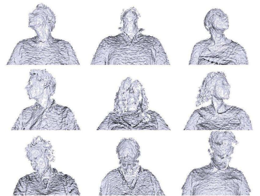
4                                                                                                  Gabriele Fanelli et al.

lighting changes and a bias towards the average face.        combine several weak classifiers into a 3D facial land-
The complexity of the modeling is an additional is-          mark detector. Ju et al. [34] detect the nose tip and the
sue. Moreover, these methods perform poorly on unseen        eyes using binary neural networks, and propose a 3D
identities [31] and cannot handle low-resolution images      shape descriptor invariant to pose and expression.
well.                                                             The authors of [73] propose a 3D Statistical Facial
    In recent years, there has been a shift towards meth-    Feature Model (SFAM), which models both the global
ods based on independent local feature detectors [61,        variations in the morphology of the face and the local
1, 3]. Such detectors are discriminative models of im-       structures around the landmarks. The low reported er-
age patches centered around the facial landmarks, often      rors for the localization of 15 points in scans of neutral
ambiguous because the limited support region cannot          faces come at the expense of processing time: over 10
cope with the large appearance variations present in the     minutes are needed to process one facial scan. In [48],
training samples. To improve accuracy and reduce the         fitting the proposed PCA shape model containing only
influence of wrong detections, global models of the fa-      the upper facial features, i.e., without the mouth, takes
cial features configuration like pictorial structures [27,   on average 2 minutes per face.
23] or Active Shape Models [20] are needed.                       In general, prior work on facial feature localization
    3D Facial Features. Similar to the 2D case, meth-        from 3D data is either sensitive to occlusions, especially
ods focusing on facial feature localization from range       of the nose, requires prior knowledge of feature map
data can be subdivided into categories using global or       thresholds, cannot handle large rotations, or does not
local information. Among the former class, the authors       run in real time.
of [46] deform a bi-linear face model to match a scan of
an unseen face in different expressions. Yet, the paper’s
focus is not on the localization of facial feature points    3 Random forest framework for face analysis
and real time performance is not achieved. Also Kaka-
diaris et al. [35] non-rigidly align an annotated model to   In Section 3.1 we first summarize a general random for-
face meshes. Constraints need to be imposed on the ini-      est framework [7], then give specific details for face anal-
tial face orientation, however. Using high quality range     ysis based on depth data in Sections 3.2 and 3.3.
scans, Weise et al. [67] presented a real time system,
capable of tracking facial motion in detail, but using
personalized templates. The same approach has been           3.1 Random forest
extended to robustly track head pose and facial defor-
mations using RGB-depth streams provided by com-             Decision trees [8] can map complex input spaces into
mercial sensors like the Kinect [65].                        simpler, discrete or continuous output spaces, depend-
    Most works that try to directly localize specific fea-   ing on whether they are used for classification of re-
ture points from 3D data take advantage of surface           gression purposes. A tree splits the original problem
curvatures. For example, the authors of [60, 55, 12] all     into smaller ones, solvable with simple predictors, thus
use curvature to roughly localize the inner corners of       achieving complex, highly non-linear mappings in a very
the eyes. Such an approach is very sensitive to missing      simple manner. A non-leaf node in the tree contains a
depth data, particularly for the regions around the in-      binary test, guiding a data sample towards the left or
ner eye corners, frequently occluded by shadows. Also        the right child node. The tests are chosen in a supervised-
Mehryar et al. [42] use surface curvatures by first ex-      learning framework, and training a tree boils down to
tracting ridge and valley points, which are then clus-       selecting the tests which cluster the training such as to
tered. The clusters are refined using a geometric model      allow good predictions using simple models.
imposing a set of distance and angle constraints on the          Random forests are collections of decision trees, each
arrangement of candidate landmarks. Colbry et al. [15]       trained on a randomly sampled subset of the available
use curvature in conjunction with the Shape Index pro-       data; this reduces over-fitting in comparison to trees
posed by [22] to locate facial feature points from range     trained on the whole dataset, as shown by Breiman [7].
scans of faces. The reported execution time of this an-      Randomness is introduced by the subset of training ex-
chor point detector is 15 sec per frame. Wang et al. [64]    amples provided to each tree, but also by a random
use point signatures [14] and Gabor filters to detect        subset of tests available for optimization at each node.
some facial feature points from 3D and 2D data. The              Fig. 1 illustrates a random regression forest map-
method needs all desired landmarks to be visible, thus       ping feature patches extracted from a depth image to a
restricting the range of head poses while being sensitive    distribution stored at each leaf. In our framework, these
to occlusions. Yu et al. [72] use genetic algorithms to      distributions model the head orientation (Section 3.2)
Random forests for real time 3D face analysis                                                                                     5

                                                                   –   acquire annotated training data P,
                                                                   –   define binary tests φ,
                                                                   –   define a measure H (P),
                                                                   –   define a distribution model to be stored at the leaves.
                                                                  These issues are discussed in the following sections.

                                                                  3.2 Head pose estimation

                                                                  3.2.1 Training data
Fig. 1 Example of regression forest for head pose estima-
tion. For each tree, the tests at the non-leaf nodes direct an    Building a forest is a supervised learning problem, i.e.,
input sample towards a leaf, where a real-valued, multivari-      training data needs to be annotated with labels on
ate distribution of the output parameters is stored. The forest
combines the results of all leaves to produce a probabilistic
                                                                  the desired output space. In our head pose estimation
prediction in the real-valued output space.                       setup, a training sample is a depth image containing
                                                                  a head, annotated with the 3D locations of a specific
                                                                  point, i.e., the tip of the nose, and the head orienta-
or locations of facial features (Section 3.3). In the fol-        tion. Fix-sized patches are extracted from a training
lowing, we outline the general training approach of a             image, each annotated with two real-valued vectors:
random forest and give the application specific details           While θ 1 = {θx , θy , θz } is the offset computed between
in Sections 3.2 and 3.3.                                          the 3D point falling at the patch center and the nose
    A tree T in a forest T = {Tt } is built from a set of         tip, the head orientation is encoded as Euler angles,
annotated patches, randomly extracted from the train-             θ 2 = {θya , θpi , θro }. In order for the forest to be more
ing images: P = {Pi }, where Ii is the appearance of the          scale-invariant, the size of the patches can be made de-
patch. Starting from the root, each tree is built recur-          pendent on the depth (e.g., at its center), however, in
sively by assigning a binary test φ(I) → {0, 1} to each           this work we assume the faces to be within a relatively
non-leaf node. Such test sends each patch (according to           narrow range of distances from the sensor.
its appearance) either to the left or right child, in this             In order to deal with background like hair and other
way, the training patches P arriving at the node are              body parts, fixed-sized patches are not only sampled
split into two sets, PL (φ) and PR (φ).                           from faces but also from regions around them. A class
    The best test φ∗ is chosen from a pool of randomly            label ci is thus assigned to each patch Pi , where ci = 1
generated ones ({φ}): all patches arriving at the node            if it is sampled from the face and 0 otherwise. The set
are evaluated by all tests in the pool and a predefined           of training patches is therefore given by P = {Pi =
information gain of the split IG (φ) is maximized:                (Ii , ci , θ i )}, where θ = (θ 1 , θ 2 ). Ii represents the image
                                                                  features Iif computed from a patch Pi . Such features
φ∗ = arg max IG (φ)                                        (1)    include the original depth values plus, optionally, the
            φ
                           X                                      geometric normals, i.e., for a depth pixel d(u, v), the
IG (φ) = H (P) −                 wi H (Pi (φ)) ,           (2)    average of the normals of the planes passing through
                       i∈{L,R}                                    d(u, v) and pairs of its 4-connected neighbors. The x, y,
where wi =      |Pi (φ)|
                     is the ratio of patches sent to each         and z coordinates of the normals are treated as separate
                  |P|
child node and H (P) is a measure of the patch cluster            feature channels.
P, usually related to the entropy of the clusters’ labels.
The measure H (P) can have different forms, depending             3.2.2 Binary tests
on whether the goal of the forest is regression, classifi-
cation, or rather a combination of the two. The mea-              Our binary tests φf,F1 ,F2 ,τ (I) are defined as:
sures that are relevant for face analysis are discussed                   X                      X
                                                                  |F1 |−1   I f (q) − |F2 |−1        I f (q) > τ,               (3)
in Sections 3.2 and 3.3. The process continues with the
                                                                          q∈F1                    q∈F2
left and the right child using the corresponding train-
ing sets PL (φ∗ ) and PR (φ∗ ) until a leaf is created when       where f is the feature channel’s index, F1 and F2 are
either the maximum tree depth is reached, or less than            two asymmetric rectangles defined within the patch,
a minimum number of training samples are left.                    and τ is a threshold. We use the difference between the
    In order to employ such a random forest framework             average values of two rectangular areas as in [25, 19],
for face analysis from depth data, we have to                     rather than single pixel differences as in [29] in order to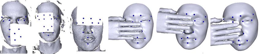
6                                                                                                                Gabriele Fanelli et al.

                                                                     defined by Equation (2), we use the measure Hc (P) of
                                                                     the cluster’s class uncertainty, defined as the entropy:
                                                                                    K
                                                                                    X
                                                                     Hc (P) = −           p (c = k|P) log (p (c = k|P)) ,              (6)
                                                                                    k=0

                                                                     where K = 1. The class probability p (c = k|P) is ap-
                                                                     proximated by the ratio of patches with class label k in
Fig. 2 Example of a training patch (larger, red rectangle)
                                                                     the set P.
with its associated offset vector (arrow) between the 3D point           The two measures (5) and (6) can be combined in
falling at the patch’s center (red dot) and the ground truth         different ways. One approach, as in the work of Gall et
location of the nose (marked in green). The two rectangles           al. [29], is to randomly select one or the other at each
F1 and F2 represent a possible choice for the regions over
which to compute a binary test, i.e., the difference between
                                                                     node of the trees, denoted in the following as the in-
the average values computed over the two boxes.                      terleaved method. A second approach (linear ) was pro-
                                                                     posed by Okada [49], i.e., a weighted sum of the two
                                                                     measures:
be less sensitive to noise; the additional computation is

                                                                     Hc (P) + α max p c = 1| P − tp , 0 Hr (P) .          (7)
negligible when integral images [63] are used. Tests de-
fined as Equation (3) represent a generalization of the              When minimizing (7), the optimization is steered by
widely-used Haar-like features [51]. An example test is              the classification term alone until the purity of posi-
shown in Figure 2: A patch is marked in red, containing              tive patches reaches the activation threshold tp . From
the two regions F1 and F2 defining the test (in black);              that point on, the regression term starts to play an ever
the arrow represents the 3D offset vector (θ 1 ) between             important role, weighted by the constant α, until the
the 3D patch center (in red) and the ground truth loca-              purity reaches 1. In this case, Hc = 0 and the optimiza-
tion of a feature point, the nose tip in this case (green).          tion is driven only by the regression measure Hr .
                                                                         In [26], we proposed a third approach, where the
3.2.3 Goodness of split                                              two measures are weighted by an exponential function
                                                                     of the depth:
A regression forest can be applied to head pose estima-                                    d
tion from depth images containing only faces [25]; in                Hc (P) + (1 − e− λ )Hr (P) ,                                      (8)
this case, all training patches are positive (ci = 1 ∀i)
                                                                     where d is the depth of the node in the tree. In this
and the measure H (P) is defined as the entropy of
                                                                     way, the regression measure is given increasingly higher
the continuous patch labels. Assuming θ n , where n ∈
                                                                     weight as we descend deeper in the tree towards the
{1, 2}, to be realizations of 3-variate Gaussians, we can
                                                                     leaves, with the parameter λ specifying the steepness
represent the labels in a set P as p(θ n ) = N (θ n ; θ n , Σ n ),
                                                                     of the change.
and thus compute the differential entropy H(P)n for n:
                                                                         Note that, when only positive patches are available,
                                                                     Hc = 0, i.e., Equations (7) and (8) are both propor-
            1
                       3

                                                                     tional to the regression measure Hr alone, and both
H(P)n =       log (2πe) |Σ n | .                             (4)
            2                                                        lead to the same selected test φ∗ , according to Equa-
We thus define the regression measure:                               tion (1).
         X                  X                                            In our experiments (see Section 4.2.2), we evaluate
Hr (P) =     log (|Σ n |) ∝   H(P)n .                        (5)     the three possibilities for combining the classification
             n                  n
                                                                     measure Hc and the regression measure Hr for training.
Substituting Equation (5) into Equation (2) and max-
imizing it actually favors splits which minimize the co-             3.2.4 Leaves
variances of the Gaussian distributions computed over
all label vectors θ n at the children nodes, thus intu-              For each leaf, the class probabilities p c = k| P and
itively decreasing the regression uncertainty.                       the distributions of the continuous head pose parame-
    Goal of the forest, however, is not only to map image            ters p(θ 1 ) = N (θ 1 ; θ 1 , Σ 1 ) and p(θ 2 ) = N (θ 2 ; θ 2 , Σ 2 )
patches into probabilistic votes in a continuous space,              are stored. The distributions are estimated from the
but, as in [26], also to decide which patches are actually           training patches that arrive at the leaf and are used for
allowed to cast such votes. In order to include a measure            estimating the head pose as explained in the following
of the classification uncertainty in the information gain            section.
Random forests for real time 3D face analysis                                                                                    7

                                     (a)                                              (b)

Fig. 3 (a) Example votes, casted by different patches. The green, red, and blue patch are classified as positives and therefore
cast votes for the nose position (correspondingly colored spheres). On the other hand, the black patch at the shoulder is
classified as negative and does not vote. (b) Example test image: the green spheres represent the votes selected after outliers
(blue spheres) are filtered out by mean shift. The large green cylinder stretches from the final estimate of the nose center in
the estimated face direction.

3.2.5 Testing                                                    for the mean shift, we use a sphere with a radius de-
                                                                 fined as one sixth of the radius of the average face in
When presented with a test depth image, patches are              the model of [52]. A cluster is declared as a head if it
densely sampled from the whole image and sent down               contains a large enough number of votes. Because the
through all trees in the forest. Each patch is guided by         number of votes is directly proportional to the number
the binary tests stored at the nodes, as illustrated in          of trees in the forest (a tree can contribute up to one
Fig. 1. A stride parameter controls how densely patches          vote for each test patch), and because the number of
are extracted, thus easily steering speed and accuracy           patches sampled is inversely proportional to the square
of the regression.                                               of the stride, we use the following threshold:

     The probability p c = k| P stored at the leaf judges
how informative the test patch is for class k. This prob-            #trees
                                                                 β           .                                                (10)
ability value tells whether the patch belongs to the head            stride2
or other body parts. Since collecting all relevant neg-
                                                                 For our experiments, we use β = 300.
ative examples is harder than collecting many positive
                                                                    For each cluster left, i.e., each head detected, the
examples, we only consider leaves with p c = k| P = 1.
                                                                 distributions left are averaged, where the mean gives
For efficiency and accuracy reasons, we also filter out
                                                                 an estimate for the position of the nose tip θ 1 and the
leaves with a high variance, which are less informative
                                                                 head orientation θ 2 and the covariance measures the
for the regression, i.e., all leaves with tr Σ 1 greater

                                                                 uncertainty of the estimates.
than a threshold maxv . The currently employed thresh-
old (maxv = 400) has been set based on a validation
set. Although the two criteria seem to be very restric-
tive, the amount of sampled patches and leaves is large          3.3 Facial features localization
enough to obtain reliable estimates.
                                                                 Since the framework for head pose estimation is very
     The remaining distributions are used to estimate
                                                                 general and can be used in principle for predicting any
θ 1 by adding the mean offsets θ 1 to the patch center
                                                                 continuous parameter of the face, the modifications for
θ 1 (P):
                                                                 localizing facial features are straightforward. Instead of
                                                                 having only two classes as in Section 3.2.1, we have
N (θ 1 ; θ 1 (P) + θ 1 , Σ 1 ).                           (9)    K + 1 classes, where K is the number of facial feature
                                                                 points we wish to localize. The set of training patches
    The corresponding means for the position of the              is therefore given by P = {Pi = (Ii , ci , θ i )}, where
nose tip are illustrated in Fig. 3. The votes are then           θ i = {θ 1i , θ 2i , . . . θ K
                                                                                              i } are the offsets between the patch
clustered, and the clusters are further refined by mean          center and the 3D locations of each of the K feature
shift in order to remove additional outliers. As kernel          points. Accordingly, (5) is computed for the K fiducials
8                                                                                                      Gabriele Fanelli et al.

and (6) is computed for the K + 1 classes, where c = 0
is the label for the background patches.
    The testing, however, slightly differs. In Section 3.2.5,
all patches are allowed to predict the location of the
nose tip and the head orientation. While this works for
nearly rigid transformations of the head, the location of
the facial features depends also on local deformations
of the face, e.g., the mouth shape. In order to avoid a
bias towards the average face due to long distance votes
that do not capture local deformations, we reduce the
influence of patches that are more distant to the fidu-
cial. We measure the confidence of a patch P for the            Fig. 4 Sample images from our synthetically generated
location of a feature point n by                                training set. The heads show large 3D rotations and varia-
                 !                                              tions in the distance to the camera and also in identity. The
         kθ n k2                                                red cylinder attached to the nose represents the ground truth
exp −              ,                                   (11)     face orientation.
           γ

where γ = 0.2 and θ n is the average offset relative to
point n, stored at the leaf where the patch P ends.             camera and further perturbed the first 30 modes of the
Allowing a patch to vote only for feature points with           PCA shape model sampling uniformly within ±2 stan-
a high confidence, i.e., above a feature-specific thresh-       dard deviation from the mean, thus introducing varia-
old, our algorithm can handle local deformations bet-           tions also in identity2 .
ter, as our experiments show. The final 3D facial feature
                                                                    Such a dataset was automatically annotated with
points’ locations are obtained by performing mean-shift
                                                                the 3D coordinates of the nose tip and the applied rota-
for each point n.
                                                                tions, represented as Euler angles. Figure 4 shows a few
                                                                of the training faces, with the red cylinder pointing out
4 Evaluation                                                    from the nose indicating the annotation in terms of nose
                                                                position and head direction. Note that the shape model
In this section, we thoroughly evaluate the proposed            captures only faces with neutral expression and closed
random forest framework for the tasks of head pose es-          mouth. Furthermore, important parts of the head like
timation from high quality range scans (Section 4.1),           hair or the full neck are missing. This will be an is-
head pose estimation from low quality depth images              sue in Section 4.2, where we discuss the limitations of
(Section 4.2), and 3D facial features localization from         synthetic training data.
high resolution scans (Section 4.3). Since the acquisi-             For testing, we use the real sequences of the ETH
tion of annotated training data is an important step            Face Pose Range Image Data Set [10]. The database
and a challenge task itself, we first present the used          contains over 10K range images of 20 people (3 females,
databases1 in each subsection.                                  6 subjects recorded twice, with and without glasses)
                                                                recorded using the scanner of [66] while turning their
                                                                head around, trying to cover all pitch and yaw rota-
4.1 Head pose estimation - high resolution                      tions. The images have a resolution of 640x480 pixels,
                                                                and a face typically consists of around 150x200 pixels.
4.1.1 Dataset                                                   The heads undergo rotations of about ±90 ◦ yaw and
                                                                ±45 ◦ pitch, while no roll is present. The data was an-
The easiest way to generate an abundance of training            notated using person-specific templates and ICP track-
data with perfect ground truth is to synthesize head            ing, in a similar fashion as what will be later described
poses. To this end, we synthetically generated a very           in 4.2.1 and shown in Figure 15. The provided ground
large training set of 640x480 range images of faces by          truth contains the 3D coordinates of the nose tip and
rendering the 3D morphable model of [52]. We made               the vector pointing from the nose towards the facing
such model undergo 50K different rotations, uniformly           direction.
sampled from ±95 ◦ yaw, ±50 ◦ pitch, and ±20 ◦ roll.
We also randomly varied the model’s distance from the
                                                                 2
                                                                    Because of the proprietary license for [52], we cannot
    1
   Most of the datasets are publicly available at http://       share the above database. The PCA model, however, can be
www.vision.ee.ethz.ch/datasets.                                 obtained from the University of Basel.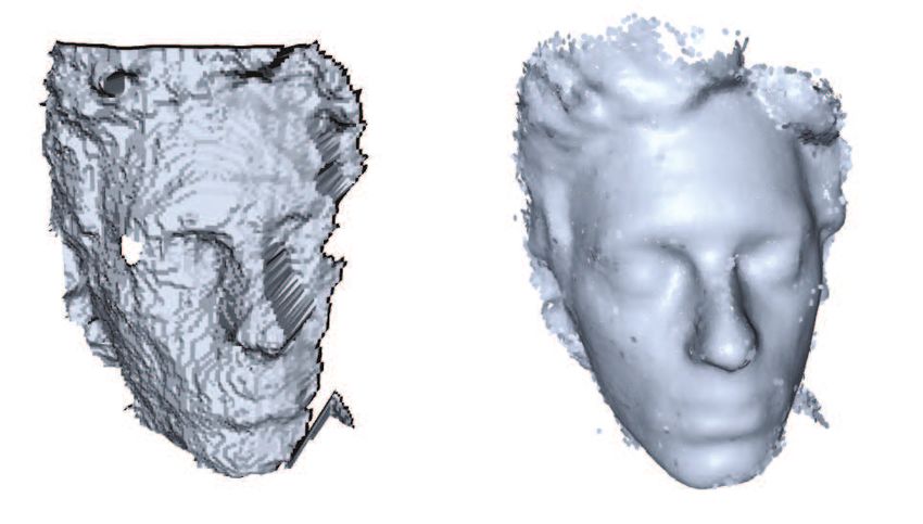
Random forests for real time 3D face analysis                                                                                                                                                            9

                                                                            100                                    40                           100                                       5
4.1.2 Experiments                                                                                                                                                          success rate
                                                                                                                                                                           miss rate
                                                                                                                                                 98                                       4
                                                                             90                                    30

                                                                                                                                   Accuracy %
                                                               Accuracy %
In this section, we assume a face to be the prominent

                                                                                                                                                                                              Missed %
                                                                                                                        Missed %
                                                                                                                                                 96                                       3
                                                                                           success rate
                                                                             80                                    20
object in the image. That means that all leaves in a                                       miss rate
                                                                                                                                                 94                                       2

tree contain a probability p (c = 1|P) = 1 and thus all                      70                                    10
                                                                                                                                                 92                                       1
patches extracted from the depth image will be allowed                                                                                           90                                    0
                                                                             60                                     0
                                                                              40   60      80      100      120   140                             500   1000     1500 2000 2500      3000
to vote, no matter their appearance.                                                    Patch size (pixels)                                                    # training images

    Training a forest involves the choice of several pa-                                    (a)                                                                  (b)
rameters. In the following, we always stop growing a
                                                              Fig. 5 (a) Success rate of the system depending on the
tree when the depth reaches 15, or if there are less than     patch size (when using 1000 training samples), overlaid to
20 patches left for training. Moreover, we randomly gen-      the missed detection rate. (b) Success and missed detection
erate 20K tests for optimization at each node, i.e., 2K       rate depending on the number of training data (for 100x100
different combinations of f , F1 , and F2 in Equation (3),    patches). Success is defined for a nose error below 20 mm and
                                                              angular error below 15 degrees.
each with 10 different threshold τ . Other parameters in-
clude the number of randomly selected training images,
the number of patches extracted from each image (fixed        of the patch. The plot shows that a minimum size for
to 20), the patch size, and the maximum size of the sub-      the patches is critical since small patches can not cap-
patches defining the areas F1 and F2 in the tests (set to     ture enough information to reliably predict the head
be half the size of the patch). Also the number of fea-       pose. However, there is also a slight performance loss
ture channels available is an important parameter; in         for large patches. In this case, the trees become more
the following, we use all features (depth plus normals)       sensitive to occlusions and strong artifacts like holes
unless otherwise specified.                                   since the patches cover a larger region and overlap more.
    A pair of crucial test-time parameters are the num-       Having a patch size between 80x80 and 100x100 pix-
ber of trees loaded in the forest and the stride control-     els seems to be a good choice where the patches are
ling the spatial sampling of the patches from an input        discriminative enough to estimate the head pose, but
image. Such values can be intuitively tuned to find the       they are still small enough such that an occlusion affects
desired trade-off between accuracy and temporal effi-         only a subset of patches. Figure 5(b) also shows accu-
ciency of the estimation process, making the algorithm        racy and missed detections rate, this time for 100x100
adaptive to the constraints of different applications.        patches, as a function of the number of training images.
    In all the following experiments, we use the Eu-          It can be noted that the performance increases with
clidean distance in millimeters as the nose localization      more training data, but it also saturates for training
error. For what concerns the orientation estimation, the      sets containing more than 2K images. For the following
ETH database does not contain large roll variations,          experiments, we trained on 3000 images, extracting 20
and in fact these rotations are not encoded in the di-        patches of size 100x100 pixels from each of them.
rectional vector provided as ground truth. We therefore           In all the following graphs, red circular markers con-
evaluated our orientation estimation performance com-         sistently represent the performance of the system when
puting the head direction vector from our estimates of        all available feature channels are used (i.e., depth plus
the yaw and pitch angles and report the angular error         geometric normals), while the blue crosses refer to the
in degrees with the ground truth vector.                      results achieved employing only the depth channel.
    Figure 5 describes the performance of the algorithm           The plots in Figure 6 show the time in milliseconds
when we varied the size of the training patches and the       needed to process one frame, once loaded in the RAM.
number of samples used for training each tree. In Fig-        The values are reported as a function of the number of
ure 5(a), the blue, continuous line shows the percentage      trees used and of the stride parameter. The numbers
of correctly classified images as a function of the patch     were computed over the whole ETH database, using
size, when 1000 training images are used. Success is de-      an Intel Core i7 CPU @ 2.67GHz processor, without
clared if the nose error is smaller than 20 mm and the        resorting to multithreading. Figure 6(a) plots the aver-
angular error is below 15 degrees. Although this mea-         age run time for a stride fixed to 10 pixels as a function
sure might be too generous for some applications, it          of the number of trees, while in Figure 6(b) 20 trees are
reflects the relative estimation performance of the ap-       loaded and the stride parameter changes instead. For
proach and is therefore a useful measure for comparing        strides equal to 10 and greater, the system always per-
different settings of the proposed approach. The red,         forms in real time. Unless otherwise specified, we use
dashed line shows instead the percentage of false posi-       these settings in all the following experiments. Obvi-
tives, i.e., missed detections, again varying with the size   ously, having to compute the normals (done on the CPU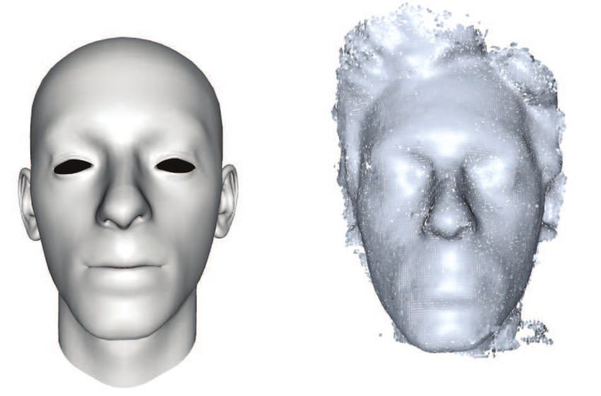
10 Gabriele Fanelli et al.
60 60 11 11
Avg angle error (degrees)
Avg angle error (degrees)
depth depth depth depth
depth+normals depth+normals 10 depth+normals 10 depth+normals
Time (ms)
Time (ms)
40 40 9 9
8 8
20 20 7 7
6 6
0 0 5 5
5 10 15 20 25 5 10 15 20 5 10 15 20 25 5 10 15 20
#Trees (stride 10) Stride (20 trees) #Trees (stride 10) Stride (20 trees)
(a) (b) (a) (b)
Fig. 6 Processing time: a) Regression time as a function of Fig. 8 Mean errors (degrees) for the orientation estimation
the number of trees in the forest when the stride is fixed to task, as a function of the number of trees in the forest (a)
10 pixels. b) Run time for a forest of 20 trees as a function of and of the stride (b).
the stride parameter.
depth depth formation. The plots show also the success rate of the
16 16
Avg nose error (mm)
Avg nose error (mm)
depth+normals depth+normals method of [10], applied to the same data3 ; their algo-
14 14
rithm uses information about the normals to generate
12 12 nose candidates, but not for refining the pose estimation
10 10
on the GPU, where a measure based on the normalized
sum of squared depth differences between reference and
8 8
5 10 15 20
#Trees (stride 10)
25 5 10 15
Stride (20 trees)
20 input range image is used.
(a) (b) Our approach proves better at both the tasks of nose
tip detection and head orientation estimation. We im-
Fig. 7 Mean errors (in millimeters) for the nose localization prove over the state-of-the-art especially at low thresh-
task, as a function of the number of trees in the forest (a) olds, which are also the most relevant. In particular, for
and of the stride (b).
a threshold of 10 mm on the nose localization error, our
improvement is of about 10% (from 63.2% to 73.0%),
using a 4-neighborhood) increases processing time, but, and even better for a threshold of 10 degrees on the an-
for the high-quality scans we are dealing with, the boost gular error: Our system succeded in 94.7%, compared
in accuracy justifies the loss in terms of speed, as can to 76.3% of Breitenstein et al.
be seen in the next plots. Table 1 reports mean and standard deviation of the
errors, compared to the ones of [10]. The first columns
Figure 7(a) shows the average errors in the nose lo-
show mean and standard deviation for the Euclidean
calization task, plotted as a function of the number of
error in the nose tip localization task, the orientation
trees when the stride is fixed to 10, while in Figure 7(b)
estimation task, and for the yaw and pitch estimation
20 trees are loaded and the stride is changed. Similarly,
errors taken singularly. The last two columns give the
the plots in Figures 8(a) and 8(b) present the average
percentages of correctly estimated images for a thresh-
errors in the estimation of the head orientation. When
old on the angular error of 10 degrees, and on the nose
comparing Figures 6, 7, and 8, we can conclude that it is
localization error of 10 millimeters. The average errors
better to increase the stride than reducing the number
were computed from the ETH database, where our sys-
of trees when the processing time needs to be reduced.
tem did not return (i.e., no cluster of votes large enough
Using normals in addition also improves the detection
was found) an estimate in 0.4% of the cases, while the
performance more than increasing the number of trees.
approach of Breitenstein failed 1.6% of the time; only
In particular, using depth and normals with a stride of
faces where both the systems returned an estimate were
10 gives a good trade-off between accuracy and process-
used to compute the average and standard deviation
ing time for our experimental settings.
values.
In Figure 9, the plots show the accuracy of the sys- Figure 10 shows the success rate of the system ap-
tem computed over the whole ETH database, when plied to the ETH database (using 20 trees and a stride
both depth and geometric normals are used as features. of 10) for an angular error threshold of 15 ◦ and a nose
Specifically, the curves in Figure 9(a) and Figure 9(b) error threshold of 20 mm. The heat map shows the
represent the percentage of correctly estimated depth database divided in 15 ◦ × 15 ◦ bins depending on the
images as functions of the success threshold set for the head’s pitch and yaw angles. The color encodes the
nose localization error, respectively for the angular er- amount of images in each bin, according to the side
ror. Using all the available feature channels performs
consistently better than relying only on the depth in- 3
We used the source code provided by the authors.Random forests for real time 3D face analysis 11
100 100
Accuracy % 90 90
Accuracy %
80 80
70 RF depth+normals 70 RF depth+normals
RF depth only RF depth only
[Breitenstein et al. 08] [Breitenstein et al. 08]
60 60
10 12 14 16 18 20 22 24 26 28 30 10 11 12 13 14 15 16 17 18 19 20
Nose error (mm) 20 trees, stride 10 Angle error (degrees) 20 trees, stride 10
(a) (b)
Fig. 9 Accuracy: (a) Percentage of correctly estimated poses as a function of the nose error threshold. (b) Accuracy plotted
against the angle error threshold. The additional information coming from the normals (red curves) consistently boosts the
performance. The black curve represents the accuracy of [10] on the same dataset.
Nose error Direction error Yaw error Pitch error dir. (≤ 10 ◦ ) nose (≤ 10 mm)
Random Forests 9.6 ± 13.4 mm 5.7 ± 8.6 ◦ 4.4 ± 2.7 ◦ 3.2 ± 2.7 ◦ 94.7% 73.0%
Breitenstein 08 10.3 ± 17.5 mm 9.1 ± 12.6 ◦ 7.0 ± 13.4 ◦ 4.8 ± 4.9 ◦ 76.3% 63.2%
Table 1 Comparison of our results with the ones of [10]. Mean and standard deviation are given for the errors on nose
localization, direction estimation, and singularly for yaw and pitch angles. The values in the last two columns are the percentages
of correctly estimated images for a threshold on the angular error of 10 degrees, and on the nose localization error of 10
millimeters. We used a forest with 20 trees, leveraging both depth and normals as features, testing with a stride of 10 pixels.
−45
1 1 .91 .83 1 1 1 1 1 .65
300
−30
.68 .76 .81 .85 .82 .99 1 .99 .88 .97 .99 .95 250
Pitch (degrees)
−15
1 .93 .92 .96 .96 .99 1 .99 .98 1 1 .99 200
0
1 1 .96 .99 1 1 1 1 .99 1 1 .98 150
15
100
1 1 1 1 1 1 1 1 1 .97 .97
30 50
1 1 1 1 1 1 1 1 1 1
45 0
−90−75−60−45−30−15 0 15 30 45 60 75 90
Yaw (degrees)
Fig. 10 Normalized success rates of the estimation, equiv-
alent of Figure 10 in [10]. The database was discretized in
15 ◦ × 15 ◦ areas and the accuracy computed for each range Fig. 11 Correctly estimated poses from the ETH database.
of angles separately. The color encodes the number of images Large rotations, glasses, and facial hair do not pose major
falling in each region, as explained by the side bar. Success is problems in most of the cases. The green cylinder represents
declared when the nose error is below 20 mm and the angular the estimated head rotation, while the red ellipse is centered
error is below 15 degrees. on the estimated 3D nose position and scaled according to
the covariance provided by the forest (scaled by a factor of
10 to ease the visualization).
color bar. The results are 100% or close to 100% for
most of the bins, especially in the central region of the the estimated nose tip location and scaled according
map, which is where most of the images fall. Our re- to the covariance output of the regression forest. The
sults are comparable or superior to the equivalent plot green cylinder stretches from the nose tip along the es-
in [10]. timated head direction. Our system is robust to large
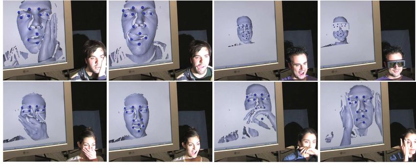
Figure 11 shows some successfully processed frames rotations and partial facial occlusions (note the girl at
from the ETH database. The red ellipse is placed on the bottom right, with most of the face covered by hair,12 Gabriele Fanelli et al.
Fig. 14 Example frames from our real time head pose estimation system, showing how the regression works even in the
presence of partial occlusions. notably of the nose. Facial expressions also can be handled to a certain degree, even though we
trained only on neutral faces.
[10]) would completely fail. Some degree of facial dy-
namics also does not seem to cause problems to the
regression in many cases, even though the synthetic
training dataset contains only neutral faces; only very
large mouth movements like yawning result in a loss of
Fig. 12 Example frames from a sequence acquired with the accuracy.
3D scanner of [66]. Occlusions (even of the nose ) and facial Some example failures are rendered in Figure 13.
expressions can be handled by our system. Note how the red ellipse is usually large, indicating a
high uncertainty of the estimate. These kind of results
are usually caused by a combination of large rotations
and missing parts in the reconstruction, e.g., because
of hair or occlusions; in those circumstances, clusters
of votes can appear in the wrong locations and if the
number of votes in them is high enough, they might be
erroneously selected as the nose tip.
4.2 Head pose estimation - low resolution
4.2.1 Dataset
Fig. 13 Example failure images from the ETH database. The To train and test our head pose estimation system on
large ellipse denotes a high variance for the estimate of the low quality depth images coming from a commercial
nose location.
sensor like the Kinect, synthesizing a database is not an
easy task. First of all, such a consumer depth camera
is built specifically for being used in a living-room en-
which is not reconstructed by the scanner). Additional vironment, i.e., capturing humans with their full body.
results are shown in Figure 12, demonstrating how the This means that heads are always present in the image
proposed algorithm can handle a certain degree of facial together with other body parts, usually the torso and
expression and occlusion, maintaining an acceptable ac- the arms. Because regions of the depth image differ-
curacy of the estimate. ent than the head are not informative about the head
We ran our real time system on a Intel Core 2 Duo pose, we need examples of negative patches, e.g., com-
computer @ 2GHz, equipped with 2GB of RAM, which ing from the body, together with positive patches ex-
was simultaneously used to acquire the range data as tracted from the face region. Lacking the human body
explained in [66]. Figure 14 shows some example frames model and MoCap trajectories employed by [57], we re-
from the video4 . Our method successfully estimates the sorted to record a new database using a Kinect. The
head pose even when the nose is totally occluded and dataset comprises 24 sequences of 20 different subjects
thus most of the other approaches based on 3D (e.g., (14 men and 6 women, 4 people with glasses) recorded
4
www.vision.ee.ethz.ch/~gfanelli/head_pose/head_ while sitting about 1 meter away from the sensor. All
forest.html subjects rotated their heads trying to span all possibleRandom forests for real time 3D face analysis 13
template
integration fitting tracking
scan model personalized template
Fig. 15 Automatic pose labeling: A user turns the head in front of the depth sensor, the scans are integrated into a point
cloud model and a generic template is fit to it. The personalized template is used for accurate rigid tracking.
ranges of yaw and pitch angles, but also some roll is
present in the data.
To label the sequences with the position of the head
and its orientation, we processed the data off-line with
a state-of-the-art template-based head tracker [65]5 , as
illustrated in Figure 15. A generic template was de-
formed to match each person’s identity as follows. First,
a sequence of scans of the users’ neutral face recorded Fig. 16 Example frames from the Biwi Kinect Head Pose
from different viewpoints were registered and fused into Database. Both depth and RGB images are present in the
one 3D point cloud as described by [68]. Then, the dataset, annotated with head poses. In this paper, we only
use the depth images for the head pose estimation algorithm.
3D morphable model of [52] was used, together with
graph-based non-rigid ICP [38], to adapt the generic
face template to the point cloud. Each sequence was
thus tracked with the subject’s template using ICP [4],
obtaining as output for each frame the 3D location of
the head (and thus of the nose tip) and the rotation
angles.
Using such automatic method to acquire the ground
truth for our database allowed us to annotate over 15K
frames in a matter of minutes. Moreover, we found that
the mean translation and rotation errors were around
1 mm and 1 degree respectively. Please note that such Fig. 17 Training patches extracted from the annotated
depth images of the Biwi Kinect Head Pose Database ac-
personalized face model is only needed for labeling the quired with a Microsoft Kinect. The green box represents a
training data: Our head pose estimation system does positive patch, while the red one is an example of a nega-
not assume any initialization phase nor person-specific tive patch. The dark dots on the face represent the model’s
training, and works on a frame-by-frame basis. vertices used to define the patch label: Only if the center of
the patch falls near such vertices, the patch is considered as
The resulting Biwi Kinect Head Pose Database con- positive.
tains head rotations in the range of around ±75 ◦ for
yaw, ±60 ◦ for pitch, and ±50 ◦ for roll. Faces are 90x110
pixels in size on average. Besides the depth data which Pose Database, we labeled them as positive only if the
we used for our algorithm, the corresponding RGB im- Euclidean distance between the 3D point falling at the
ages are also available, as shown in Figure 16. center of the patch and the closest point on the face
model used for annotation was below 10 millimeters.
4.2.2 Experiments In this way, negative patches were extracted not only
from the torso and the arms, but also from the hair.
Training patches must now be distinguished between Figure 17 shows this process.
positives (extracted from the head region) and nega-
In the following experiments, unless explicitly men-
tives (belonging to other body parts). When we ran-
tioned otherwise, all training and testing parameters
domly extracted patches from the Biwi Kinect Head
are kept the same as in the previous evaluation done
5
Commercially available: http://www.faceshift.com on high resolution scans. We only reduce the size of the14 Gabriele Fanelli et al.
100 15 int 100 100
Missed detections %
λ=2
95 λ=5 95 95
Accuracy %
Accuracy %
Accuracy %
10 λ = 10
90 int lin 90 int 90 int
λ=2 λ=2 λ=2
λ=5 5 λ=5 λ=5
85 85 85
λ = 10 λ = 10 λ = 10
lin lin lin
80 0 80 80
300 350 400 450 500 300 350 400 450 500 10 12 14 16 18 20 22 24 26 28 30 10 12 14 16 18 20 22 24 26 28 30
Max variance Max variance Nose error (mm) Angle error (degrees)
(a) (b) (a) (b)
Fig. 18 Accuracy (a) of the tested methods as a function of Fig. 19 Accuracy for the nose tip estimation error (a), re-
the maximum variance parameter, used to prune less infor- spectively the angle error (b) of the tested methods. The
mative leaves in the forest. Success is defined when the nose curves are plotted for different values of the threshold defining
estimation error is below 20mm and the thresholds for the success.
orientation estimation error is set to 15 degrees. The plots in
(b) show the percentage of images were did not return an es-
timate (false negatives), again as a function of the maximum the maxv parameter increases, i.e., as more and more
variance. It can be noted that the evaluated methods perform leaves are allowed to vote. Success means that the de-
rather similarly and the differences are small, except for the
interleaved scenario, which consistently performs worse.
tected nose tip is within 20mm from the ground truth
location, and that the angular error is below 15 ◦ . Fig-
ure 18(b) shows, again as a function of the maximum
patches to 80x80 because the heads are smaller in the leaves’ variance, the percentage of missed detections.
Kinect images than in the 3D scans. Furthermore, we In general, low values of the parameter maxv have a
extract 20 negative patches per training image in addi- negative impact on the performance, as the number
tion to the 20 positive patches. For testing, patches end- of votes left can become too small. However, reduc-
ing in a leaf with p c| P < 1 and tr Σ 1 ≥ maxv are
ing the maximum variance makes only the most cer-
discarded. Given the much lower quality of the depth re- tain votes pass, producing better estimates if there are
construction, using the geometric normals as additional many votes available, e.g., when the face is covering
features does not bring any improvement to the esti- a large part of the image; moreover, reducing maxv
mation, therefore we only use the depth channel in this can also be used to speed up the estimation time. The
section. Because the database does not contain a uni- parameter shows how well the different schemes mini-
form distribution of head poses, but has a sharp peak mize the classification and regression uncertainty. Be-
around the frontal face configuration, as can be noted cause only the leaves with low uncertainties are used
from Figure 21, we bin the space of yaw and pitch an- for voting, trees with a large percentage of leaves with
gles and cap the number of images for each bin. a high uncertainty will yield a high missed detection
In Section 3.2.3, we described different ways to train rate, as shown in Figure 18(b). In this regards, all tested
forests capable of classifying depth patches into head methods appear to behave similarly, except for the in-
or body and at the same time estimating the head pose terleaved scenario, which consistently performs worse,
from the positive patches. In order to compare the dis- indicating that the trees produced using such method
cussed training strategies (interleaved, linear, and ex- had leaves with higher uncertainty. We also note that
ponential ), we divided the database into a testing and the exponential weighting scheme with λ = 5 returns
training set of respectively 2 (persons number 1 and 12) the lowest number of missed detections.
and 18 subjects. The plots in Figures 19(a) and 19(b) show the suc-
Depending on the method used to combine the clas- cess rate as function of a threshold on the nose error,
sification and regression measures, additional parame- respectively on the orientation error. We note again
ters might be needed. In the interleaved setting [29], the lower accuracy achieved by the interleaving scheme,
each measure is chosen with uniform probability, except while the other methods perform similarly.
at the two deepest levels of the trees where the regres- We performed a 4-fold, subject-independent cross-
sion measure is always used. For the linear weighting validation on the Biwi Kinect Head Pose Database, us-
approach (7), we set α and tp as suggested by [49], ing an exponential weighting scheme with λ set to 5. All
namely to 1.0 and 0.8. For the exponential weighting other parameters were kept as described earlier. The re-
function based on the tree depth (8), we used λ equal sults are given in Table 2, where mean and standard de-
to 2, 5, and 10. All comparisons were done with a forest viation of the nose tip localization, face orientation es-
of 20 trees and a stride of 10. timation, yaw, pitch and roll errors are shown together
Results are plotted in Figures 18 and 19. The suc- with the percentage of missed detections and the aver-
cess rate of the algorithm is shown in Figure 18(a), as age time necessary to process an image, depending onYou can also read