Sound quality of side-by-side vehicles: Investigation of multidimensional sensory profiles and loudness equalization in an industrial context
←
→
Page content transcription
If your browser does not render page correctly, please read the page content below
Acta Acustica 2021, 5, 7
Ó A. Benghanem et al., Published by EDP Sciences, 2021
https://doi.org/10.1051/aacus/2020032

                                                                                                                        Available online at:
                                                                                                         https://acta-acustica.edpsciences.org

    SCIENTIFIC ARTICLE

Sound quality of side-by-side vehicles: Investigation of multidimensional
sensory profiles and loudness equalization in an industrial context
Abdelghani Benghanem1,2,*, Olivier Valentin1,2, Philippe-Aubert Gauthier2,3, and Alain Berry1,2
1
  Groupe d’Acoustique de l’Université de Sherbrooke, 2500 Boul. de l’Université, Sherbrooke, J1K 2R1 Québec, Canada
2
  Centre for Interdisciplinary Research in Music, Media, and Technology, McGill University, 527 Sherbrooke St. West,
  Montréal, H3A 1E3 Québec, Canada
3
  École des Arts Visuels et Médiatiques, Université du Québec à Montréal, 405, rue Sainte-Catherine Est, Montréal,
  H2L 2C4 Québec, Canada

            Received 3 January 2020, Accepted 15 December 2020

            Abstract – The sensory perception of products influences the relationship of potential users or buyers with
            these products. Sound quality is part of this sensory experience and is critical for products such as sports or
            utility vehicles as the sound conveys the impression of power or efficiency, among others. Therefore, there is
            a need to provide tools based on scientific methodology to acoustical engineers designing such vehicles. The
            motivation of this work was the need to explore new and faster methods for quicker and simpler sound quality
            evaluation. In this paper, the sound quality of side-by-side utility vehicles is investigated using the rapid sen-
            sory profile measurement method, and then by creating virtual participants using bootstrapping methods.
            Additionally, this study also investigates the effect of loudness equalization of the sound samples used during
            the listening tests. Results from these studies were used to establish the sensory profiles, desire-to-buy values
            and desirable sound profiles regarding the tested vehicles. Equalized loudness tests provide a finer sensory pro-
            file than those obtained using non-equalized sound samples. Furthermore, statistical analysis results confirm
            that adding virtual participants to the original data using a bootstrapping approach helps highlighting key
            information without altering the validity of the results.

            Keywords: Sound quality, Sensory profiles, Loudness equalization, Bootstrap, Sound design

1 Introduction                                                              partment. The vehicle can be used to transport loads in its
                                                                            dump box (tools, parts, furniture, materials such as earth,
    The sounds of consumer products influence the general                    sand, and so on.) and to move trailers. These vehicles are
perception of these products. This is particularly important                also equipped with a cabin that allows the passenger
for vehicle interior sound and therefore for vehicle manufac-               compartment to be closed to improve user comfort in
turers who wish to attach a positive impression to their                    cold or bad weather [2]. Because they are often used for
products and to improve users satisfaction. In this vein,                   heavy works, the sensation of power is important for the
the field of sound quality has been expanding rapidly in                     customers and makers, a sensation that can be communi-
the past decades [1]. Sound quality is even more significant                 cated through sound, hence the present work. For 95% of
for sport or utility vehicles as their sounds should either                 usage time, these vehicles are used at constant speed for
convey sportiveness or an impression of power or efficiency.                 transportation.
In this paper, we are interested in understanding the per-                      This study is part of a larger applied research project
ceived sound quality of side-by-side vehicles (SSV).                        that combines physical and perceptual studies of these vehi-
    The SSVs are four-wheel drive recreational vehicle of                   cles with an industrial partner. The specific context for this
the utility type. They are called side-by-side because they                 work also adds practical constraints, develop and test a
usually have two seats beside each other. Such vehicles                     rapid, less time-consuming, pragmatic, workflow for sound
are used to work on farms or in forests in rugged terrain,                  quality studies in realistic industrial context where quick
among other things. SSVs are designed to carry a driver                     answers are required in order to adapt the acoustical design
and a passenger seated on his right and are equipped                        in a yearly cycle of design and fabrication. Therefore, part
with a dump body, located at the rear of the passenger com-                 of our contribution is based on testing the following
                                                                            research aim in a realistic heavily constrained context.
*Corresponding author: Abdelghani.Benghanem@USherbrooke.ca                  The specific expectations of the industrial partner are
This is an Open Access article distributed under the terms of the Creative Commons Attribution License (https://creativecommons.org/licenses/by/4.0),
              which permits unrestricted use, distribution, and reproduction in any medium, provided the original work is properly cited.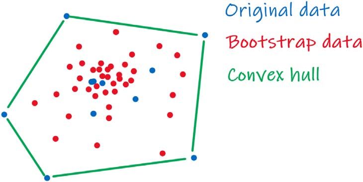
2                                      A. Benghanem et al.: Acta Acustica 2021, 5, 7

threefold and define the research aims: (1) to identify a fas-     technique, participants are asked to evaluate a series of
ter yet rigorous way to achieve sensory profiling of SSVs          sound attributes one after the other. This method has sev-
sound based on consumers’ perceptions, interpretations            eral advantages over the semantic differential as well: (1)
and their expectations, (2) to investigate the effect of loud-    there is no need to construct bipolar scales (avoiding diffi-
ness equalization of the sound samples on sensory profiles,        culties in choosing contrasting adjectives that really belong
and (3) to determine if using virtual participants can            to the same dimension) and (2) different adjectives can be
improve the analysis of the information contained in the          used for describing the same dimension (e.g., loud and soft
original perceptive evaluations conducted on a limited sam-       or near and far), thus providing data for homogeneity and
ple of participants. Such approach would undoubtedly help         reliability analyses [7].
to facilitate the integration of sound quality studies in the         Either way, one of the first steps is to define the attri-
general acoustical engineering workflow at a lower cost,           butes. Lists of perceptual attributes and terms are well
but also within a more agile and flexible paradigm to ensure       defined for sound and audio evaluations but most of the
quick and real impact on the work of acoustical engineers.        time, specific sound products are studied, which therefore
    Subsections hereafter present a relevant state of the art,    requires appropriate attributes [15, 16]. Unfortunately,
as well as some essential knowledge on sound quality,             there is a lack of standardized lists of attributes to accu-
required to undertake the scientific motivations and the           rately describe the sound characteristics perceived by SSV
methodology.                                                      regular consumers [17, 18]. Yet, two methods might be use-
                                                                  ful to overcome this limitation: (1) consensus vocabulary
1.1 Sound quality and sound signature                             development procedures or (2) individual vocabulary devel-
                                                                  opment procedures.
    Blauert and Jekosch [3] define sound quality as follows:
Product sound quality is a descriptor of the adequacy of the      1.2 Rapid sensory profiling
sound attached to a product. It results from judgments
upon the totality of auditory characteristics of the said             Sensory profiling, initially used in the food and wine
sound, the judgments being performed with reference to            industry, focuses on the five senses and their impact on
the set of those desired features of the product which are        the consumer experience [19–22]. Sensory analysis methods
apparent to the users in their actual cognitive, actional         to describe and to quantify the perceptual characteristics of
and emotional situation. In many experiments, researchers         audio stimuli have been actively researched in recent years.
have investigated the acoustic sound quality of the interior      A classical sensory profile includes the following key steps:
noise of vehicles using perceptual evaluations and physical       (a) firstly, the selection, training and supervision of a short
measurements [1, 4–6]. Several perceptual evaluations of          panel of assessors, (b) the generation of attributes that
vehicle sound studies consider a single attribute, the most       describe the similarities and differences between products,
popular is the annoyance. This is so because the experi-          (c) the determination and consensus on the evaluation pro-
menters already have an idea of which sound property is           cedure for each of the selected attributes, (d) the training
related to the sound quality they want. However, it is            for the evaluation and scaling of the selected attributes
known that sound quality is multidimensional and the over-        for stimuli, and (e) finally the quantitative evaluation of
all judgment depends on a limited set of perceptual attri-        stimuli, in a randomized presentation. This conventional
butes [7–9]. In addition, it is clear that each vehicle           method, well defined in the literature, is considered the
category (sport, recreational, utility, etc.) has a specific       most reliable sensory profiling method. From a practical
sound signature.                                                  point of view, it is easy to use and communicate. However,
    The sound signature can be defined as the sensory pro-         the specificity of the automotive industry makes the use of
file of a sound resulting from listening test responses giving     the conventional profiling difficult. There are several issues
judgments about the various perceptual attributes. This           that render it less effective: time consuming, expensive,
can be achieved in numerous ways. The semantic differen-          need of dedicated resources, and the fact that this method
tial (SD) technique [10] still seems to be one of the most fre-   is not adapted to reveal inter-individual differences. For
quently used methods to investigate sounds from a                 example, to apply such an approach, it takes about 6
perceptual point of view in different situations. Typically,      months with a 3-h session per week with experts, which gen-
for SD the concept (here sound perception/sensation) is           erates astronomical costs. Thus, companies cannot afford to
scaled on a set of successive pairs of adjectives, such as        repeat this experience for every product or element, espe-
pleasant–unpleasant, smooth–rough, loud–soft, using a             cially for an annual design cycle and agile revision of acous-
7-point rating scale [7, 11]. Often, Von Bismarck’s semantic      tical engineering on a regular basis. Quick methods for a
differential scales are chosen as a reference [12]. However,      quick turnaround are mandatory to ensure a full penetra-
instead of using pairs of bipolar adjectives (e.g. dull–sharp)    tion of sound quality methods within the industrial sector.
as in the traditional differential semantic paradigm, some        This is a primary motivation for this work, being able to ful-
studies [13] rather use an attribute and its negation (e.g.       fill the industrial sector pragmatical realities [21, 23, 24].
sharp–not sharp) as proposed by Kendall and Carterette            For instance, Bergeron et al. [25] applied the classical sen-
[14].                                                             sory profile technique to obtain a description of internal
    Another method, called multidimensional scaling has           rolling noise of automobiles, using quantitative perceptual
been applied to several sound quality studies. In this            criteria. Despite the overall success of such a method for
A. Benghanem et al.: Acta Acustica 2021, 5, 7 3
studying vehicle sound quality, this approach has a major The methodology employed for the experiment reported
limitation, the long implementation time: the training of herein is inspired from the flash profiling approach. In this
the participants and the consensus vocabulary phase paper, this promising method is adapted to quantify and
require a total of 36 h. rapidly assess both the sound signature and sound quality
Therefore, new sensory characterization methodologies of SSVs. This method is supposed to provide accurate
called rapid sensory profiling methods were developed, for results, similar to the results provided by conventional
the food and the flavour industry, to avoid training sessions, descriptive analysis, with a light implementation.
and as a substitute to the classical method. These method-
ologies are less time consuming, more flexible and can be 1.3 Participatory sound design
used with semi-qualified assessors and even consumers, pro-
viding sensory mapping that is very close to a classical The second objective of this research is tightly inter-
descriptive analysis with highly qualified panels [19, 26]. twined with a sound design perspective. As product sound
Lorho [8], used a descriptive analysis method [24], to com- quality is defined as the adequacy of the sound attached
pare the perceptual characteristics of spatial improvement to a product, it is dependent on user expectations and con-
systems for sound reproduction on headphones. The experi- text. Sound design deals with the engineering of sound and
menter used the individual vocabulary development a central concept is the communication that takes place
approach. This approach proved to be faster compared to when using the product [31]. Sound design aims to create
traditional consensus vocabulary methods, and the attribute or modify the timbre of product sounds to meet specific
test produced reasonable results in terms of perceptual intentions [32].
description and algorithm discrimination. Lokki et al. [9] Indeed, many sound quality studies focus on existing
used a similar approach to obtain perceptual attributes sounds or virtual sounds in the listening tests [33]. One
(and perceptual profiles) for the evaluation and acoustic question related to participatory research and participatory
comparison of concert halls. That study demonstrated that engineering is how the end-user or consumer can be
such a method works well to assess subjective differences with included in the sound design process with a rigorous and sci-
respect to concert halls and seating positions in the same hall. entific method. Consequently, we investigated the idea of
Kaplanis et al. [27] used a rapid sensory analysis, the integrating sound design profiling to classical sound quality
flash profile [23], to examine the perceptual properties of listening tests. On this matter, it is clear from the literature
automotive audio systems. The flash profile method requires that part of sound design changes is related to sound qual-
only three sessions: (a) a first one for the generation of attri- ity outcomes [34, 35]. Nevertheless, the participants (e.g.,
butes, ((b) one for the setting up of lists of attributes, and users, consumers) already have an idea of the sound profile
(c) a last one for the quantitative evaluation of stimuli. Flash they want. This paper reports an attempt for potential con-
profiling allows the perceptual experience to be evaluated sumers to design their own ideal sound profile. For the SSV
using the attributes developed during the individual elicita- manufacturer, this is an important aspect as it will help in
tion phase in a time-efficient manner. However, it has been the further design stage for sound quality and product ame-
shown that the free elicitation method used in the individual lioration. More precisely, it will help in identifying the direc-
vocabulary process is more difficult for untrained partici- tion in which acoustical engineers should work.
pants than for assessors familiar with descriptive analysis
methods. Lorho [8] proposed to use the grid-directory tech- 1.4 Effect of global loudness equalization on sensory
nique in the attribute elicitation process for assessors who profiles
are not familiar with descriptive analysis. For example, for
the generation of verbal descriptors for quality assessment There is a constant debate between academics and
of perceived spatial perception of an audio system, Berg industry, shall listening tests for vehicle sound quality be
and Rumsey opted for the grid-directory technique [28]. based on global loudness-equalized sound samples or not?
Thus, this research highlighted the need for clear definitions Albeit this might seem like an obvious question, for a vehicle
and avoiding ambiguous attributes. manufacturer interested in enhanced sound quality, it is not.
Le Bagousse et al. [29] conducted an exclusively lexical Indeed, the current industrial and legislative context
study (without listening to sound) to reduce the number imposes reduced sound pressure levels (SPL) to vehicle man-
of terms by classifying them into categories. Then, they ufacturers. Therefore, reducing the SPL is always a desirable
integrated these categories to assess the perceived sound avenue in this context. Indeed, levels are still very important
quality for several audio coding algorithms for digital audio factors in daily acoustical engineering in order to respect the
data compression applications. Additional publications noise legislation. The balance between SPL reduction and
related to sensory analysis applied to acoustics can be found timber adjustment for sound quality is therefore a recurring
in the literature: Wankling et al. [26] research interests source of debate among the practicing acoustical engineers.
include the development of subjective descriptors to assess Accordingly, on the one hand, conducting listening tests
the perceived quality of low-frequency audio reproduction with sounds that have not been loudness equalized and
in small rooms. Mattila’s research work [30] is related to leading to a conclusion that a change in loudness/SPL is
the descriptive analysis of sound quality of transmitted desirable would not be helpful. On the other hand, conduct-
speech in the context of mobile communications, using ing listening tests with loudness–equalized sounds somehow
the semantic differentiation method [10]. denatures the tested sounds or products. Based on that dual4 A. Benghanem et al.: Acta Acustica 2021, 5, 7
position, there is a need to investigate the effect of loudness
equalization on sound quality experiments. Few hints along
these lines exist in the current literature [36–38].
Parizet et al. [36] evaluated perceptual prominent fac-
tors on sound perception for noises recorded in a high-speed
train, with sounds at their real levels, and then with sounds
equalized in loudness. The results of this study were that:
(1) the first influencing factor of interior noise perception
is loudness of the signal. The influence of loudness is quite
the same for every listener, and loudness is mainly due to Figure 1. Conceptual illustration of bootstrapped data in two-
dimension space. The boot-strapped points (red) lie within (or
the speed of the train and (2) when the influence of loudness
on) the convex hull (green) of the original data (blue).
is eliminated, the perception is different among listeners.
Most of them (70%) prefer the noise to be in the low fre-
quency range while some other listeners choose opposite pool of actual participants [41–43]. In this trend, we inves-
preference. However, it should be pointed out that in this tigated the application of the bootstrapping methods [41] to
second case, the experimenters failed to develop a predictive sound quality studies. To the authors’ knowledge, this has
model of preference based on existing psychoacoustic not been examined for sound quality studies. The question
descriptors using these data. Susini et al. [37] evaluated then being: does bootstrapping facilitate the interpretation
the influence of loudness on sound recognition based on of the results and does it agree with results obtained from
an explicit memory experiment. The results of this study more established methods?
revealed that recognition scores were significantly different Bootstrapping is a family of methods based on random
when sounds are presented with the same or different SPL sampling with replacement of a given data set to virtually
between the study phase and the test phase; recognition increase the number of observations. In other words, boot-
was significantly better when target sounds are presented strap approaches are likely to generate data similar to the
with the same typical level in the study phase and in the observed data. For instance, in this study, assuming the case
test phase. of N observations (listeners) of A attributes for the sound
Since most studies suggest that loudness affects sound sample i and condition b stored in a data matrix Xb,i 2 RN A ,
quality, studies in sound quality systematically equalize bootstrapping would involve M re-sampling lines of Xb,i
sound samples in global loudness to help test participants with replacement leading to an augmented data matrix
focusing on finer details rather than the obvious overall per- X0 b;i 2 RMA . Several properties of the bootstrapping
ceived loudness [39]. For instance, Kwon et al. [40] proposed method in relation with this work and the implemented pro-
a model of psychoacoustic sportiveness for vehicle interior cedure are worth mentioning. First, bootstrapping will lead
sound excluding the effect of loudness. The model for psy- to mean values equivalent to the mean of the original data.
choacoustic sportiveness was determined as a function of Second, the confidence interval on the statistical estimates
roughness, sharpness, and tonality. However, there are only will be smaller. Third, the bootstrapping re-sampled points
a limited number of studies of vehicle sounds in the litera- in a A-dimension space will lie within the A-dimension
ture that compare the two approaches (i.e. loudness–equal- convex hull [44] of the original data set (see Fig. 1).
ized or not) [38]. Besides these works, the question remains Indeed, the implementation of the bootstrap is of little
open for SSVs. All in all, considering the fact that the differ- value when the statistical inference can be made by classical
ent methods and specific types of sounds condition used in analytical methods, for which the conditions of application
each study affect the results, this needs more investigation. are met. It is therefore not intended to replace conventional
Therefore, an experiment was set up to prove to SSVs statistical inference methods where these are applicable, but
manufacturers that the global sound equalization of sounds rather to provide answers to questions for which conven-
affects the sensory profiles and this can be demonstrated tional methods are inapplicable or unavailable. However,
more precisely with two listening test sessions based on for the principal component analysis based on the variance
the same sound samples and exact same methodology (in- of data, the use of the bootstrap is a valid alternative to
cluding hardware, participants, and conditions). To do so, greatly improve the readability of the data [45].
in the first test, sound samples were presented at their real
loudness levels, and in the second test, the global loudness 1.6 Principal component analysis
of sound samples was equalized.
In sensory profiling, several attributes are studied simul-
1.5 Bootstrap taneously. However, it is difficult to represent simultane-
ously and simply such a large number of quantitative
The fourth objective of this research is related to the size variables in a simple graph, because the data are no longer
of available data and the required time for sound quality represented in a two-dimensional space but in a larger
studies. Testing sounds with actual customers or experts dimensional space whose interpretation is more difficult.
takes time and resources. One of the scientific questions is Moreover, it is important to retain the most meaningful
how the analysis of results can be enhanced using a method uncorrelated attributes. The multivariate statistical analy-
to simulate a pool of virtual participants based on a limited sis tools answers these questions and reveals the hiddenA. Benghanem et al.: Acta Acustica 2021, 5, 7 5
structure of the data. The principle is to project the 12
responses of the participants in the listening tests onto V1, N: 82.1 sone V5, N: 18 sone
the principals components (PC) dimensional space. 10 V2, N: 49.7 sone V6, N: 53.2 sone
Specific loudness N'
In this regard, the chosen statistical tool for this study is V3, N: 62.2 sone V7, N: 118 sone
8 V4, N: 70.5 sone
the Principal Component Analysis (PCA). The main objec-
tive of the PCA is to reduce the dimensionality of a data set
6
consisting of a large number of interdependent variables,
while maintaining as much as possible the variation present 4
in the initial data-set. Besides reducing the number of
dimensions, the PCA enables identifying insignificant or 2
unreliable data, thus de-noising the data. Exhaustive infor-
mation on PCA can be found in [46–48]. 2 4 6 8 10 12 14 16 18 20 22 24
Band no
1.7 Research objectives
Figure 2. Specific loudness N0 as a function of frequencies on
The aim of this work was based on the need to identify the Bark scale and global loudness N (in the legend) of the seven
and adapt rapid sensory methods to the sound quality of vehicles for the left binaural channel for the constant speed
SSV, using the reliable resources already available, and ver- condition.
ify the effectiveness of this method. As the flash profiling
approach seems to be easy to implement in sound quality Next, all sound samples of each driving condition were
context, this method was adapted in an attempt to quickly global-loudness equalized approximately to 29.3 sone for
assess sensory profiles of SSV sounds from a consumers’ the idle condition, 49.9 sone for the constant speed, and
point of view. Since participatory sound design approach 48.9 sone for the acceleration.
seems to be less time-consuming than the regular method, To illustrate the loudness differences, an example of the
this approach was used to facilitate the sound design pro- specific and global loudness for the seven sound samples of
cess. Even if it has been previously investigated in the liter- the constant speed condition is shown in Figure 2. In this
ature, it is of interest to confirm if equalizing the overall case, the sound samples were equalized in global loudness
loudness reduces the correlation between scores of percep- in comparison to the global loudness of the V2 sample
tual attributes in sensory profiles. To avoid multiple time (red line). The global loudness values were calculated
consuming sessions, the rapid sensory method was therefore according to the ISO532B model. The equalization was
chosen to investigate this research question. The equalized applied iteratively by applying a linear gain on the sound
and non-equalized cases are compared with the same condi- to be equalized. This gain adjustment allows the global
tions, participants, hardware and method. Finally, it was loudness (the area under these graphs) to be the same as
also of interest to investigate if bootstrapping can be used for the red line with a threshold of 0.25 sone. This equaliza-
as a solution to overcome the limitation regarding the par- tion is done for both channels (left and right) in a single pro-
ticipants number. Thus, these points respond to the litera- cess with a single gain (same for left and right, in order to
ture review, and are the contributions of this paper. preserve the binaural sound image).
As a result, for each driving condition, two versions of
sound stimuli were produced. Using these stimuli, two sim-
2 Method ilar perceptual test sessions were organized with the same
2.1 Sound samples panel of participants: a first session with sounds played
back at actual sound pressure levels, and a second session
Seven recreational side-by-side vehicles were considered with sounds with the same global loudness.
in this study. The interior sounds of the vehicles were Sound stimuli were presented to participants on SENN-
recorded using a binaural GRAS KEMAR Head and Torso HEISER headphones (chosen among models HD600,
Simulator (model 45BB) equipped with large ears and HD555, HD598, or HD579). Each headphone was fre-
40AD 1/200 GRAS microphones, with a sampling frequency quency-equalized by filtering each sound sample with
of 48 kHz and a 24-bit resolution. appropriate frequency response amplitude-only for the left
To establish the sound signature of each vehicle, we con- and right channels of each headset, using 2048-order zero-
sidered the following three driving conditions: (1) idle (1200 phase finite impulse response filters. This creates the same
rpm), (2) constant speed (30 km/h), and (3) wide open output signals from the headphones as those measured with
throttle (WOT) acceleration (0–60 km/h). These condi- the binaural mannequin. Then, short fade-ins and fade-outs
tions were chosen for different reasons. The idle condition were applied in the beginning and at the end of each sound
reflects the customer’s first impression of the sound signa- sample so that they could be repeated without audible arti-
ture of the parked vehicle. The constant speed condition facts. The total duration of each sample was 5 s. A valida-
was chosen as 95% of the operating time is at velocities tion of sound reconstruction was performed: the binaural
below 30 km/h for these vehicles. The acceleration condi- microphones were installed on the KEMAR mannequin
tion reflects the sensation associated with vehicle (equipped with the same artificial ears specified above) with
sportiveness. the binaural headsets and the spectrum of the sounds6 A. Benghanem et al.: Acta Acustica 2021, 5, 7
recorded on the mannequin was compared with the spec- synonyms were eliminated among the chosen descriptors
trum of the original sounds measured in the interior of and those deemed the most important were selected among
the vehicle cabin in operating condition. the remaining descriptors: Firstly, the panel grouped similar
words together, e.g. Power with Powerful and Vibration
2.2 Participants with Vibrating. Then, all words were quickly examined to
group synonyms and antonyms together, in a simple way
A jury of 20 individuals (17 males, 3 females) between according to the panel’s common understanding. Here are
23 and 54 years of age participated to the study. All partic- a few examples of words grouped together: Regular synonym
ipants were users of recreational products similar to the of Constant, Performing synonym of Powerful, and Weak
studied SSVs and all of them had hearing thresholds below antonym of Powerful. Otherwise, when the group discussion
25 dB HL (hearing level). The participants’ hearing thresh- tended to diverge on a word, it was left as it was, so as not to
olds have been measured using an online hearing test1 influence individuals on their understanding of the words.
before the beginning of the listening tests. This study was For example, bass versus high-pitched. We have to keep in
reviewed and approved by the Comité d’éthique pour la mind that participants are just SSV users and not experts
recherche, the Internal review Board at Université de in sensory analysis. For most of them, this is the first time
Sherbrooke, Québec, Canada. Informed consent was they were participating to such a study. Therefore, they
obtained from all participants before they were enrolled in probably do not have a vocabulary as developed as the
the study. Participants did not received financial compensa- experts or the acousticians. It is important to note that
tion for their participation in the tests. the group discussion was open and inclusive and was man-
aged by three experimenters, one of which coming from mar-
2.3 Step #1: Group discussion and attribute keting with experience in managing focus groups. A total of
identification 128 terms were kept at the end of this task that took approx-
The aim of the group discussion was to define the attri- imately 1 h. The perceptual attributes obtained from the
butes associated with the seven recreational vehicles accord- group discussion are presented in Table 1. This table shows
ing to sound perception. The discussion took place in a large the most recurrent descriptors (occurrence larger than 1)
room in the presence of all participants and members of the generated by the jury panel with the occurrence of each
research team. In this phase, monophonic sounds were pre- word. Note that all the tests were conducted in French.
sented using a Genelec 8040B loudspeaker. All the groups For this article, the attributes have been translated into
discussions were held in French, as the target language English using the Cambridge French–English Dictionary.
for attributes was also French. This experience was struc- Since one participant miss-understood the instructions
tured in two tasks. and made analogies with food terms, some the terms in
the footnotes are not related to sound.
2.3.1 Generation of attributes Two individual voting sessions using anonymous online
survey were then conducted. In the first vote, each partici-
The first task aimed at generating the perceptual attri- pant had to select a list of 10 attributes from the list defined
butes. A preliminary training and familiarization session previously, which they considered relevant. These 20 attri-
was included because some of the participants were not butes are assumed to be commonly used and understood by
familiar with sensory profiling. Sounds were played ran- the majority of subjects. Table 2 indicates the results of the
domly and participants freely proposed terms describing first vote session.
the various sounds. The duration of this training was about In the second vote, each participant had to select the
30 min. most important six attributes from the 10 attributes
Then, participants were asked to freely describe the retained after the first vote. Table 3 indicates the results
sound samples using verbal descriptors by entering them of the second vote session. The six attributes selected by
in an online form. The sound samples were randomly pre- the jury panel at the end of the two voting sessions are
sented (the original sounds and the sounds equalized in glo- shown in gray. At the end, the jury agreed in a consensus
bal loudness, have been mixed to form the random playlist on this short list of six sensory attributes for the quantita-
of sounds), several times with breaks, until each participant tive evaluation of SSV sounds. The attributes of this selec-
was able to generate about 10 attributes, which took about tion were then defined as the perceptual dimensions to be
45 min to complete. At the end of this phase, a total of 255 evaluated in the listening tests.
terms were collected. Then, all the descriptors generated by The two voting sessions and final consensus on six attri-
all the participants were compiled, sorted in decreasing butes took 30 min. Flash profiling is normally based on the
order of occurrence, and then shown to the panel on a large use of free choice profiling that allows participants to use
screen in front of the room. their own list of attributes. In order to facilitate the later
analysis of the results, this step was slightly modified to
2.3.2 Selection of attributes generate a common list of perceptual attributes, compared
to the standard flash profile method. The two individual
The second task aimed at selecting the most relevant
voting sessions with a brief group discussion, will make it
descriptors. Based on a group discussion, antonyms and
possible to have well-defined and common attributes for
1
https://hearingtest.online/ the entire jury panel.A. Benghanem et al.: Acta Acustica 2021, 5, 7 7
Table 1. The most recurrent French attributes (31 words). The Table 2. First vote session results. The six attributes selected in
six attributes selected in the final list are formatted in bold. the final list are formatted in bold.
Attributes English translation Occurrence Attributes English translation Votes
Puissant Powerful 20 Puissant Powerful 18
Strident Strident 14 Vibrant Vibrating 16
Doux Soft 13 Métallique Metallic 15
Sourd Deaf 9 Agressif Aggressive 14
Métallique Metallic 9 Doux Soft 13
Vibrant Vibrating 7 Mécanique Mechanical 13
Agressif Aggressive 6 Bruyant Noisy 13
Grave Bass 6 Constant Constant 12
Sillement Hissing 5 Bourdonnant Buzzing 12
Étouffé Muffled 5 Strident Strident 11
Sec Dry, curt, sharp 5 Sourd Deaf 11
Bruyant Noisy 5 Étouffé Muffled 11
Aigu High-pitched 3 Grave Bass 9
Constant Constant 3 Sifflement Whistling 8
Fade Tasteless 3 Sillement Hissing 7
Frottement Friction 3 Lourd Heavy 5
Lourd Heavy 3 Fade Tasteless 4
Sifflement Whistling 3 Sec Dry, curt, sharp 4
Mécanique Mechanical 3 Frottement Friction 3
Bourdonnant Buzzing 2 Aigu High-pitched 1
Essoufflé Breathless, puffed 2
Étourdissant Deafening 2
Feutré Felted 2 Table 3. Second vote session results. The six attributes selected
Grognement Growl 2 in the final list are formatted in bold.
Ralenti Idle 2
Onctueux Creamy, smooth 2 Attributes English translation Votes
Rapide Rapid 2 Puissant Powerful 16
Régulier Regular 2 Aggressif Aggressive 14
Résonant Resonant, echoing 2 Métallique Metallic 12
Saccadé Jerky 2 Bruyant Noisy 12
Stimulant Stimulating 2 Doux Soft 11
Descriptors occurred once (in French): Acide, Adoucissant, Vibrant Vibrating 11
Aiguiser, Aspiré, Balayeuse, Bouillonnant, Brulé, Caoutchou- Bourdonnant Buzzing 8
teux, Caverneux, Chargé, Chatouille, Claire, Commun, Com- Constant Constan 8
presseur, Confortable, Courroie, Crémeux, Crissement, Sourd Deaf 8
Croissant, Croustillant, Dépassement, Destructif, Différentiel, Étouffé Muffled 7
Élégant, Éloigner, Énergique, Ennuyeux, Envahissant, Équilibré, Mécanique Mechanical 5
Excitant, Expiration, Fatiguant, Filtré, Fondant, Fréquence,
Froid, Gouteux, Granulaire, Gronde, Grunty, Gutturale,
Huileux, Impatient, Industriel, Inégale, Insécurisant, Inspiration, loudness (Test NOEQ) and (b) with sounds equalized in
Insupportable, Intense, Irritant, Juteux, Laveuse, Lointain, global loudness (Test EQ). Participants had a 1-h break
Louvoiement, Mélanger, Mixte, Mou, Muffler, Neutre, Oscillant,
between the two tests. Each test was structured in three
Pâteux, Pétillant, Petit, Plaisant, Prêt, Progressif, Rafale,
Rampé, Râpé, Rassurant, Rauque, Réconfortant, Redondant,
experiments with an average duration of 45 min each.
Retenu, Riche, Robuste, Ronronnement, Rugueux, Rythmé,
Sablonneux, Salé, Sirène, Solide, Soufflant, Sportif, Stable, Subtil, 2.4.1 Experiment 1 – Sensory profile
Texturé, Tonnerre, Traction, Trafic, Aspirateur, Vaillant, Vent,
Ventilation, Vrombissant, Wouwouwou.
In this first experiment, the objective was to determine
the sensory profile for the sounds of the seven vehicles. Thus,
listening tests were conducted to evaluate perceptual attri-
For comparison purposes, only 3 h were needed to define butes using continuous intensity scales. The listening tests
the perceptual attributes whereas the classical method as were set up in a quiet meeting room. During the test, the
described in [25] requires twelve sessions of 3 h (36 h in participant was seated in front of a laptop screen with a
total). graphical user interface (GUI) used to play the sounds and
to give ratings, by adjusting a slider from 0 to 100, for each
2.4 Step #2: Listening tests perceptual attribute. Each participant was asked to rate
the seven sound samples for the three driving conditions
In this step, each participant performed two similar and for each of the six perceptual dimensions in Table 3.
listening tests: (a) with sounds not equalized in global An example of the user interface for this experiment is8 A. Benghanem et al.: Acta Acustica 2021, 5, 7
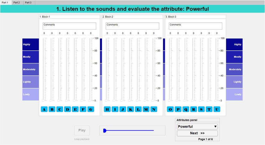
Figure 3. GUI for sound signature assessment (translated from French), presented in full-screen mode to the participants for clarity.
provided in Figure 3. Each block corresponds to a driving assigned by the individual subject for the sound (V1) in
condition. The bold letters (A–G, H–N, and O–U) are the experiment 1. Each participant gave a desired score (from
sound samples of the seven vehicles presented in random 20 to 120 points) for each perceptual attribute and for
order in each block and for each attribute. The GUI allows each of the three driving conditions (acceleration, idle and
the possibility to play the sounds back as many times constant speed). The scale was extended below 0 and
required. beyond 100 to ensure that if an attribute already received
100 (or 0) in experiment 1, it was possible to go beyond
2.4.2 Experiment 2 – Evaluation of global preference (or below).
The objective of the second experiment was to rate the 2.5 Data analysis
vehicles according to a global preference criterion. This
experiment consisted in evaluating the desire-to-purchase Before creating the sound profiles from the listening
(Envie d’achat in French) of the products by a sound rating tests, a statistical analysis was performed to demonstrate
test. In this experiment, the sounds were the same as those the statistical significance of the responses [49].
assessed in experiment 1. The participants were asked to Firstly, we performed the Shapiro–Wilk test [50] to
rate the sounds of the seven tested vehicles, according to determine if the null hypothesis of composite normality is
the desire-to-purchase, for each of the three conditions. a reasonable assumption regarding the population distribu-
The GUI used for this experiment is similar to that shown tion of each sample. The returned value of H = 0 indicates
in Figure 3 except for the evaluated attribute (desire-to- that Shapiro–Wilk test fails to reject the null hypothesis at
purchase). the 5% significance level. Thus, as the collected data did not
follow a normal distribution, Friedman’s test [51] was used
2.4.3 Experiment 3 – Participatory design of a target rather than classical ANOVA.
sound signature In this study, we considered three criteria (or three
dimensions) on which Friedman’s test was performed. In
The aim of the third experiment was to determine what each case, Friedman’s ANOVA table indicates the probabil-
users want as the preferred or target sound signature of a ity of falsely of the null hypothesis of the group on observa-
chosen reference vehicle. tions. The significance level was set to a = 0.05. The three
In this experiment, each participant was instructed to statistical criteria are as follows:
focus on the attributes previously assessed in experiment
1 and was asked to design the “best” sensory profile for 1. The group of seven vehicles: the nullity hypothesis
the reference vehicle (V1), according to their preferences. would be that the sounds of the vehicles presented
The initial ratings for each attribute in this test were those have no effect on the participants’ responses.A. Benghanem et al.: Acta Acustica 2021, 5, 7 9
Table 4. Friedman’s ANOVA test results. 2. The group of the three driving conditions: the nullity
hypothesis would be that the driving conditions pre-
Criteria p-value NOEQ p-value EQ sented have no effect on the participants’ responses.
60
Vehicles 1.78 10 3.50 107 3. The group of the six attributes evaluated: the nullity
Conditions 9.08 1031 3.46 106 hypothesis would be that the attributes presented
Attributes 1.93 107 1.40 103 have no effect on the participants’ responses.
3 Results and interpretation
100 100 3.1 ANOVA and box-plots
Scores (%)
Scores (%)
The p-values of the ANOVA are given in Table 4. For
50 50 each criteria, the p-value is smaller than the significance
level (a). This means that vehicle sounds, driving condi-
tions, and attributes have a statistically significant effect
0 0 on the response of participants.
V1 V2 V3 V4 V5 V6 V7 V1 V2 V3 V4 V5 V6 V7
Sounds Sounds To facilitate the reading, only the results for constant
speed condition are reported in this paper, as this condition
represents 95% of the operating time of these SSV.
100 100 As a representative example, Figure 4 illustrates the
responses of the participants in the listening tests, as box-
Scores (%)
Scores (%)
plots form, for the constant speed condition and sounds
50 50 not equalized in global loudness. In each box-plot diagram,
the scores in % are represented for each sound sample.
The box-plots for all participants show some outliers
0 0
V1 V2 V3 V4 V5 V6 V7 V1 V2 V3 V4 V5 V6 V7 and some wide interquartile intervals. This is probably
Sounds Sounds due to a lack of consensus in consumer responses. Also, from
Figure 4, comparisons can be made between the sound pro-
files of the seven vehicles. For the constant speed condition,
100 100
the sound of V5 is evaluated the least aggressive, the least
noisy, the softest, the least metallic, the least powerful and
Scores (%)
Scores (%)
the least vibrating. Moreover, the sound of V7 is evaluated
50 50
the most aggressive, the noisiest, the less soft, the most
metallic, the most powerful and the most vibrating.
0 0
Figure 4g presents the box-plot diagram of the evalua-
V1 V2 V3 V4 V5 V6 V7 V1 V2 V3 V4 V5 V6 V7 tion of the vehicle sounds according to desire-to-buy (the
Sounds Sounds second experiment of the listening test) for the constant
speed condition. For this condition, Figure 4g shows that
100
V2 is the preferred vehicle sound in terms of desire-to-buy
(63%).
Scores (%)
50 3.2 Sensory profiles
In this section, the current and desired sound profiles of
0
the tested vehicles are presented and compared. The sound
V1 V2 V3 V4 V5 V6 V7 signature or sound profile of each vehicle is illustrated
Sounds according to the six attributes as a radar plot. The median
values of the participants’ responses for each attribute were
used to design these sound profiles.
Figure 4. Box-plot of attributes rating (a–f) and desire-to-buy The results are displayed for original sounds without
rating (g) for constant speed condition. Test NOEQ. The x-axis global loudness equalization (Test NOEQ) and for the
represents the seven sound samples evaluated and the y-axis sounds with global loudness equalization (Test EQ).
represents the ratings in % of the participants for each attribute. Figure 5 presents the current sound profiles of the seven
The median is represented by a black dot surrounded by a
vehicles tested at constant speed.
colored circle. The 25th and 75th percentiles are presented by a
thick solid line. The thin lines added at the ends extend to the Figure 5 shows that the sensory profiles are different for
extreme values (maximum and minimum) and the outliers are the different vehicles. This suggests that the assessors were
marked as circles. The confidence interval of the median values is able to discriminate between the stimuli. Also, Figure 5
represented by triangles. (a) Powerful, (b) Aggressive, (c) shows that the sensory profiles for original sounds (solid
Metallic, (d) Noisy, (e) soft, (f) Vibrating and (g) Desire-to-buy. lines) are different to those for the sounds with global10 A. Benghanem et al.: Acta Acustica 2021, 5, 7
S 100 N S 100 N
80 80 S 100 N S 100 N
60 60 80 80
40 40 60 60
20 20 40 40
M 0 A M 0 A 20 20
M 0 A M 0 A
P V P V
P V P V
S 100 N S 100 N
80 80
60 60 Figure 6. Sensory profiles “desired” for V1 for constant-speed
40 40 condition. Solid lines: Test NOEQ. Dotted lines: Test EQ. A:
20 20
M 0 A M 0 A Aggressive, N: Noisy, S: Soft, M: Metallic, P: Powerful, V:
Vibrating. (a) V1 and (b) V1 desired.
P V P V assessors. Firstly, Figure 6 shows that the sensory profiles
desired by assessors for the reference vehicle (V1) were very
similar for EQ and NOEQ results. This is a very interesting
S 100 N S 100 N results that support the idea that a desired sound style or
80 80
60 60 signature might not so much be defined by the loudness.
40 40 For instance, as an illustrative example, a well-branded
20 20
M 0 A M 0 A car sound would sound as desirable and recognizable while
listening to a YouTube video or seeing one live in the far
distance, i.e., the recognizable signature should not be
P V P V
depend on level or perceived loudness.
Secondly, results from Figure 6b give valuable clues on
how to improve the sound signature of V1, by comparison
S 100 N with Figure 6a: the participants want a softer, less metallic,
80 more powerful and less vibrating sound profile of V1.
60
40
20 3.4 Effect of global loudness equalization on sensory
M 0 A
profiles
This section studies the effect of global loudness equal-
P V ization on sensory profiling using two listening test sessions
with and without global loudness equalization. To do so,
correlation analyses were performed to evaluate the rela-
tionship between the subjective assessment of perceptual
Figure 5. Sensory profiles for constant-speed condition. Solid
attributes and the global loudness of the sound samples.
lines: Test NOEQ. Dotted Lines: Test EQ. A: Aggressive, N:
Noisy, S: Soft, M: Metallic, P: Powerful, V: Vibrating. (a) V1, The results of these correlation analyses are presented in
(b) V2, (c) V3, (d) V4, (e) V5, (f) V6 and (g) V7. Figures 7–9 for the two listening tests. Figure 7 illustrates
the correlations between the six perceptual attributes scores
and the global loudness of each of the seven sounds. Figure 8
loudness equalization (dotted lines) except for V3 and V4 presents scatter plots of the attributes scores. Figure 9 pre-
that have close profiles. The NOEQ profiles show large vari- sents the correlations between the desire-to-buy scores and
ations of the Noisy and Soft attributes among vehicles the global loudness of each of the seven sounds.
(consider V5, V6, V7). This is expected since Noisy and Soft Table 5 presents the matrix of correlation coefficients
are likely to have a large correlation with global loudness. In (R) and the matrix of p-values (P) for testing the hypothe-
contrast, the EQ profiles show more balanced scores of all sis that there is no relationship between the observed phe-
six attributes. This suggests that the global loudness equal- nomena (null hypothesis). If an off-diagonal element of P
ization of the sound stimuli has an effect on subjective is smaller than the significance level (default is 0.05), then
assessments of perceptual attributes and thus on sensory the corresponding correlation in R is considered significant.
profiles. Figure 7a shows that for the listening tests with sound
stimuli not equalized in global loudness, all perceptual attri-
3.3 Participatory sound design butes scores were correlated with global loudness: the attri-
butes Aggressive, Noisy, Metallic, Powerful and Vibrating
Figure 6 presents the sound profile for the reference increase with global loudness (positive dependence) while
vehicle (V1) and the desired sound profile by the panel of the attribute Soft decreases with global loudness (negativeA. Benghanem et al.: Acta Acustica 2021, 5, 7 11
quantify differences in perceptual attributes scores for dif-
Loudness
100
ferent vehicles with the exception of the attributes Noisy
50
and, to some extent, Soft, which show small score disper-
0
20 60 20 60 20 60 20 60 20 60 20 60 sion. This is expected since these perceptual attributes are
Aggressive Noisy Soft Metallic Powerful Vibrating directly correlated to global loudness. It can therefore be
assumed that global loudness equalization forces the listen-
ers to do a finer analysis of the perceptual attributes. The
Loudness
100 score dispersion for the Aggressive, Metallic, Powerful,
50 Vibrating attributes is somewhat smaller for the EQ test
0 as compared to the NOEQ test, which shows that vehicle
20 60 20 60 20 60 20 60 20 60 20 60 sounds are more difficult to discriminate for EQ sounds
Aggressive Noisy Soft Metallic Powerful Vibrating with respect to those attributes. Also, the ranking of vehi-
cles with respect to those Aggressive, Metallic, Powerful,
Vibrating attributes is quite different for the EQ and
Figure 7. Scatter plots of the median scores of perceptual NOEQ tests, which shows that global loudness masks the
attributes (in %) and global loudness of sounds (in sone) for evaluation of less dominant attributes.
constant-speed condition. Legend: V1, V2, V3, V4, V5, The scatter plots in Figure 8a, show that the perceptual
V6, V7. (a) Test NOEQ and (b) Test EQ.
attributes are strongly correlated with each other in NOEQ
tests, which is expectable since the perceptual attributes
dependence). These observations are confirmed by large scores are also strongly correlated with global loudness.
correlation coefficients between global loudness and attri- Each attribute has a positive correlation with all other
butes scores: 0.96 for Aggressive, 0.98 for Noisy, 0.96 for attributes except for the attribute Soft which has a negative
Soft, 0.86 for Metallic, 0.95 for Powerful, and 0.95 for correlation with all attributes. This observation was con-
Vibrating. These values were computed using the Pearson firmed by the correlation coefficients computed between
product-moment correlation coefficient. This suggests that the perceptual attributes using the Pearson product-
global loudness dominates the sensory profiles, all percep- moment correlation coefficient. Additionally, the results in
tual attributes being proportional, or inversely propor- Figure 8b show that there is less or no correlation between
tional, to global loudness of the sounds. In contrast, perceptual attributes when the sound samples have been
Figure 7b shows that for the tests with sound stimuli equal- equalized in global loudness, with some exceptions. For
ized in global loudness, listeners were able to perceive and instance, significant correlations can be found when
Table 5. Matrix of correlation coefficients (R) and p-values (P).
Aggressive Noisy Soft Metallic Powerful Vibrating
(a) Test NOEQ
Aggressive R 1
P 1
Noisy R 0.987 1
P 0.000 1
Soft R 0.949 0.971 1
P 0.001 0.000 1
Metallic R 0.905 0.897 0.915 1
P 0.005 0.006 0.004 1
Powerful R 0.993 0.979 0.926 0.867 1
P 0.000 0.000 0.003 0.011 1
Vibrating R 0.971 0.983 0.970 0.894 0.956 1
P 0.000 0.000 0.000 0.007 0.001 1
(b) Test EQ
Aggressive R 1
P 1
Noisy R 0.800 1
P 0.031 1
Soft R 0.304 0.360 1
P 0.508 0.427 1
Metallic R 0.381 0.302 0.662 1
P 0.399 0.510 0.105 1
Powerful R 0.542 0.573 0.302 0.736 1
P 0.209 0.179 0.510 0.059 1
Vibrating R 0.687 0.477 0.005 0.493 0.842 1
P 0.088 0.279 0.992 0.261 0.017 112 A. Benghanem et al.: Acta Acustica 2021, 5, 7
80
60 Aggressive
40 100 100
Loudness
Loudness
20
80
60 Noisy 50 50
40
20
80 0 0
60 Soft
40 20 40 60 80 20 40 60 80
20
Desire-to-buy Desire-to-buy
80
60 Metallic
40
20
80 Figure 9. Scatter plots of the desire-to-buy attribute for
60 Powerful
40 constant speed. Legend: V1, V2, V3, V4, V5, V6,
20
V7. (a) Test NOEQ and (b) Test EQ.
80
60 Vibrating
40
20 These results confirm the strong dependence of the sub-
20 60 20 60 20 60 20 60 20 60 20 60 jective evaluation of the sound samples on their global loud-
ness level and suggest that global loudness equalization
reduces the correlation between perceptual attributes scores
80 of sensory profiles for the tested vehicles. In addition, based
60 Aggressive on the dispersion of the perceptual attributes scores, it can
40
20 be assumed that global loudness equalization forces listeners
80
60
to more finely differentiate the perceptual attributes. It
40 Noisy
20
should then allow for a more detailed sensory profile differ-
80
entiation. These outcomes are solidified by PCA results in
60
40 Soft Section 3.6.
20
80
60
3.5 Bootstrapping for creating virtual participants
40 Metallic
20 The above results have been obtained on a limited num-
80 ber of participants (16 for NOEQ and 19 for EQ). From the
60 Powerful
40 20 subjects who participated in the study, one had to leave
20
80 for personal reasons and three others did not answer the full
60 Vibrating test, so their answers were not considered.
40
20 The nature of sensory profiling methodology makes it
20 60 20 60 20 60 20 60 20 60 20 60 complicated, time-consuming, and costly to collect data
on larger groups.
In this paper, we rely on a simple bootstrapping proce-
Figure 8. Scatter plots of perceptual attributes for constant- dure. First, for each condition b and each sound sample i,
speed condition. The scatter plots correspond to the median one starts with the original sensory profile matrix
scores (% for each attribute) for each of the seven sounds. The Xb,i 2 R166 in the NOEQ case (Xb,i 2 R196 in the EQ
variable names displayed along the diagonal of the matrix are
case). Second, Xb,i is line-resampled uniformly at random
also the column names for labeling the x and y axes. For
instance, the top left graph is a comparison between Aggressive
sampling
0
with replacement to obtain a new data matrix
and Noisy, and so on. Legend: V1, V2, V3, V4, V5, V6, Xb;i 2 R166 for the lth resampling of Xb,i. Note that in
V7. (a) Test NOEQ and (b) Test EQ. our case the resampled data includes the N = 16 original
participants in NOEQ case (or N = 19 original participants
in EQ case). From this new data matrix X0 b;i we compute
comparing Aggressive and Noisy (0.8), or Powerful and the mean along each column leading to a new virtual partic-
0
Vibrating (0.84): this suggests that in EQ tests, partici- ipant that gives a sensory profile sl 2 R16 (which is a
pants did not make a large difference between these pairs response of the new virtual participant for sound sample i).
of perceptual attributes, in these specific cases. Indeed, This is repeated L times for the index l leading to a new pool
the strong correlation between Powerful and Vibrating in of L virtual participants. In the end, for a given condition
this study is mainly due to one stimulus (V5) which is con- and a given sound sample, the resulting sensory profile
sidered the most Powerful and most Vibrating distantly bootstrapped matrix is given by Y 2 RL6 . This new sen-
from the other 6 stimuli. This is probably due to the partic- sory profile matrix is then used in the subsequent stages
ular timbre of this sound. of analysis.
Finally, Figure 9a show that the desire-to-buy is Figure 10 illustrates the bi-plot of assessors’ evaluations
strongly correlated to the global loudness level: the desire- for two distributed perceptual attributes, for the original
to-buy scores decreases with the global loudness (negative data and bootstrapped data. The number of bootstrap
dependence). samples chosen for this analysis is L = 1000 samples. AfterYou can also read