Global atmospheric CO2 inverse models converging on neutral tropical land exchange, but disagreeing on fossil fuel and atmospheric growth rate ...
←
→
Page content transcription
If your browser does not render page correctly, please read the page content below
Biogeosciences, 16, 117–134, 2019
https://doi.org/10.5194/bg-16-117-2019
© Author(s) 2019. This work is distributed under
the Creative Commons Attribution 4.0 License.

Global atmospheric CO2 inverse models converging on neutral
tropical land exchange, but disagreeing on fossil fuel and
atmospheric growth rate
Benjamin Gaubert1 , Britton B. Stephens2 , Sourish Basu3,4 , Frédéric Chevallier5 , Feng Deng6 , Eric A. Kort7 ,
Prabir K. Patra8 , Wouter Peters9 , Christian Rödenbeck10 , Tazu Saeki11 , David Schimel12 , Ingrid Van der
Laan-Luijkx9 , Steven Wofsy13 , and Yi Yin14
1 Atmospheric   Chemistry Observations & Modeling Laboratory (ACOM), National Center for Atmospheric Research,
Boulder, CO, USA
2 Earth Observing Laboratory (EOL), National Center for Atmospheric Research, Boulder, CO, USA
3 Earth System Research Laboratory, National Oceanic and Atmospheric Administration, Boulder, CO, USA
4 Cooperative Institute for Research in Environmental Sciences, University of Colorado, Boulder, CO, USA
5 Laboratoire des Sciences du Climat et de l’Environnement, Institut Pierre-Simon Laplace, CEA-CNRS-UVSQ,

Gif sur Yvette, 91191 CEDEX, France
6 Department of Physics, University of Toronto, Toronto, Canada
7 Climate and Space Sciences and Engineering, University of Michigan, Ann Arbor, MI, USA
8 RGGC/IACE/ACMPT, Japan Agency for Marine-Earth Science and Technology (JAMSTEC), Yokohama 236 0001, Japan
9 Meteorology and Air Quality, Wageningen University, Wageningen, the Netherlands
10 Max Planck Institute for Biogeochemistry, 07745 Jena, Germany
11 Center for Global Environmental Research, National Institute for Environmental Studies, Tsukuba, Japan
12 Jet Propulsion Laboratory, California Institute of Technology, Pasadena, CA, USA
13 School of Engineering and Applied Science and Department of Earth and Planetary Sciences, Harvard University,

Cambridge, MA, USA
14 Division of Geological and Planetary Sciences, California Institute of Technology, Pasadena, CA, USA

Correspondence: Benjamin Gaubert (gaubert@ucar.edu)

Received: 20 August 2018 – Discussion started: 30 August 2018
Revised: 11 December 2018 – Accepted: 14 December 2018 – Published: 16 January 2019

Abstract. We have compared a suite of recent global CO2          REgional Carbon Cycle Assessment and Processes (REC-
atmospheric inversion results to independent airborne obser-     CAP) projects, with model spread reduced by 80 % since
vations and to each other, to assess their dependence on dif-    TransCom 3 and 70 % since RECCAP. Most modeled CO2
ferences in northern extratropical (NET) vertical transport      fields agree reasonably well with the HIPPO observations,
and to identify some of the drivers of model spread. We          specifically for the annual mean vertical gradients in the
evaluate posterior CO2 concentration profiles against obser-     Northern Hemisphere. Northern Hemisphere vertical mixing
vations from the High-Performance Instrumented Airborne          no longer appears to be a dominant driver of northern versus
Platform for Environmental Research (HIAPER) Pole-to-            tropical (T) annual flux differences. Our newer suite of mod-
Pole Observations (HIPPO) aircraft campaigns over the mid-       els still gives northern extratropical land uptake that is mod-
Pacific in 2009–2011. Although the models differ in inverse      est relative to previous estimates (Gurney et al., 2002; Peylin
approaches, assimilated observations, prior fluxes, and trans-   et al., 2013) and near-neutral tropical land uptake for 2009–
port models, their broad latitudinal separation of land fluxes   2011. Given estimates of emissions from deforestation, this
has converged significantly since the Atmospheric Carbon         implies a continued uptake in intact tropical forests that is
Cycle Inversion Intercomparison (TransCom 3) and the             strong relative to historical estimates (Gurney et al., 2002;

Published by Copernicus Publications on behalf of the European Geosciences Union.
118                    B. Gaubert et al.: Drivers of remaining differences between converging global CO2 inverse models

Peylin et al., 2013). The results from these models for other       the 11 inverse models used different inversion techniques,
time periods (2004–2014, 2001–2004, 1992–1996) and re-              atmospheric models, and observational datasets. When the
evaluation of the TransCom 3 Level 2 and RECCAP results             fluxes were analyzed for the years 2001 to 2004, Peylin et al.
confirm that tropical land carbon fluxes including deforesta-       (2013) found an overall improved consistency between inver-
tion have been near neutral for several decades. However,           sions on a large scale and over specific regions compared to
models still have large disagreements on ocean–land par-            T3L2 when the network of atmospheric sites was less dense.
titioning. The fossil fuel (FF) and the atmospheric growth          RECCAP inversions showed a general agreement on the to-
rate terms have been thought to be the best-known terms in          tal natural land carbon flux long-term mean and its interan-
the global carbon budget, but we show that they currently           nual variability over 1991–2010. The total ocean plus land
limit our ability to assess regional-scale terrestrial fluxes and   sink estimates were more robust over the NET than for the
ocean–land partitioning from the model ensemble.                    tropics and in the southern extratropics (SET). The remain-
                                                                    ing spread led to a disagreement on the NET–T–SET land
                                                                    partitioning, with some models simulating a stronger tropi-
                                                                    cal source compensated for by larger NET and SET sinks.
1   Introduction                                                    Peylin et al. (2013) also noted that the group of models that
                                                                    assimilated observations at their corresponding times rather
Current appraisals of the global atmospheric carbon budget          than using monthly means had more consistent, weaker trop-
are informed by surface fluxes computed by inverse trans-           ical sources, and weaker northern sink land fluxes.
port models (e.g., Newsam and Enting, 1988; Tans et al.,               Several additional inverse modeling intercomparison stud-
1990; Rayner et al., 1999; Gurney et al., 2002, 2003, 2004;         ies have more recently involved satellite, surface, and joint
Peylin et al., 2013). Net carbon flux to the atmosphere             surface–satellite inversion (e.g., Chevallier et al., 2014;
is derived from temporal and spatial CO2 gradients given            Houweling et al., 2015). In these studies, the inversion sys-
by atmospheric observations and prior estimates of compo-           tems used space-borne retrievals of column-average dry air-
nent fluxes and their uncertainties. This assessment of atmo-       mole fraction of CO2 (XCO2 ) from the Orbiting Carbon Ob-
spheric sources and sinks relies on (1) atmospheric tracer          servatory 2 (OCO-2) satellite since July 2014 (Eldering et al.,
transport models that link fluxes to atmospheric CO2 fields,        2017) and from the Greenhouse Gases Observing Satellite
(2) prior emissions and sinks (e.g., from process model flux        (GOSAT; Kuze et al., 2009) instrument since January 2009.
estimates), (3) the spatial and temporal representativeness         Those inverse exercises, however, are still sensitive to satel-
and coverage of the observational network, and (4) error            lite retrieval algorithms and the inversions’ prior assump-
statistics associated with each information piece. Since the        tions. In particular, the results are sensitive to systematic er-
problem is underdetermined, it is essential to quantify the         rors from transport and satellite retrievals (Houweling et al.,
uncertainty and biases of posterior fluxes and CO2 con-             2010; Chevallier, 2015).
centrations with independent observations and cross-model              Schimel et al. (2015) investigated the NET versus T+SET
comparisons. The most prominent community-wide inverse              land flux partitioning as indicated by atmospheric inversions,
result intercomparison that included comparisons of pos-            biosphere process model simulations, and forest inventory
terior concentrations to independent observations was the           estimates, and they estimated a large land uptake over the
TransCom 3 study (Gurney et al., 2002, 2004), which stud-           tropics by intact forests due to a significant CO2 fertilization
ied fluxes for the 1992–1996 period. This comparison could          effect. This study argued for the importance of comparing
focus on the impact of transport model differences by op-           posterior CO2 fields to observations, which was not done in
timizing the fluxes using a common method over the same             RECCAP, in order to fully understand and predict terrestrial
regions (11 land and 11 ocean). One particular feature of           land sinks, as well as their variation due to CO2 and climate
the seasonally resolved (Level 2) TransCom 3 inversions             feedbacks. A follow-up inversion intercomparison focused
(hereafter denoted as T3L2) was the direct dependence of            on East Asia and found that large flux adjustments were pos-
flux estimates on vertical gradients of CO2 (Stephens et al.,       sible even though models simulated the observed gradient in
2007), leading to a different partitioning between north-           vertical profiles measured by aircraft well, because the uncer-
ern extratropical (NET) versus tropical (T) land sinks.             tainties from model transport and fossil fuel (FF) prior emis-
A more recent community-wide CO2 inverse model inter-               sions were compensated for by the flux adjustments (Thomp-
comparison was carried out as part of the REgional Carbon           son et al., 2016).
Cycle Assessment and Processes project (RECCAP, http://                The          HIAPER            Pole-to-Pole          Observa-
www.globalcarbonproject.org/reccap/ last access: 7 January          tions       (HIPPO)         campaign         (Wofsy,       2011,
2019; Canadell et al., 2011). The atmospheric inversion com-        https://doi.org/10.3334/CDIAC/HIPPO_010)                 spanned
ponent of RECCAP was a comprehensive intercomparison                large latitudinal, vertical, and temporal coverage (2009
that analyzed long-term mean, long-term trend, interannual          to 2011) and provides a useful atmospheric trace gas
variations, and mean seasonal variations of CO2 fluxes using        dataset for investigating the consistency of inverse fluxes
common post-processing (Peylin et al., 2013). In RECCAP,            and posterior concentration results. Graven et al. (2013)

Biogeosciences, 16, 117–134, 2019                                                         www.biogeosciences.net/16/117/2019/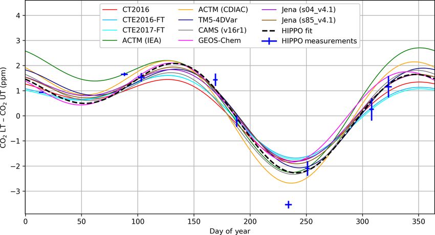
B. Gaubert et al.: Drivers of remaining differences between converging global CO2 inverse models                             119

found an increase in the CO2 seasonal amplitude by up to           transport models, wind fields, analysis procedures, and sub-
50 % at mid- to high latitudes of the Northern Hemisphere          set of assimilated observations. The atmospheric chemistry-
and at altitudes ranging between 3 and 6 km between the            transport model (ACTM) system performed two inversions
HIPPO period and the 1950s. Deng et al. (2015) compared            with different prescribed fossil fuel emissions (Saeki and
posterior CO2 and O3 fields from GEOS-Chem to the                  Patra, 2017), one based on totals from the Carbon Diox-
HIPPO observations to diagnose the impact of the upper             ide Information Analysis Center (CDIAC; Boden et al.,
troposphere and lower stratosphere (UTLS) definition on            2016) and another based on the International Energy Agency
retrieved fluxes. These results indicate a significant impact of   (IEA/OECD, 2016), which allows us to assess sensitivity
transport errors on retrieved fluxes. Frankenberg et al. (2016)    to the FF prior only. This is also the case for the two Car-
evaluated the CarbonTracker CT2013B and Monitoring                 bonTracker Europe versions, CTE2016-FT (Fast Track) and
Atmospheric Composition and Climate (MACC) v13r1                   CTE2017-FT, where only the subset of observations and the
atmospheric inverse models, as well as satellite retrievals        FF prior are different (van der Laan-Luijkx et al., 2017).
from GOSAT, TES (Tropospheric Emission Spectrometer),                 It is worth noting that some inverse models are con-
and AIRS (Atmospheric Infrared Sounder) in comparison to           structed in a similar framework. Some share the same trans-
HIPPO measurements. They found that, despite an overall            port model, such as TM5 that is used in four inversions, and
agreement between inversions and HIPPO measurements,               some use the same meteorological fields. Five inverse sys-
systematic model transport errors remain important.                tems nudge their forecast field to the ERA-Interim reanaly-
   After years of continuous model development, the goal of        sis (Dee et al., 2011). The two longest flux estimates, from
this study is to investigate whether global inverse models         CAMS (v16r1) and Jena (s85_v4.1), are used to reproduce
are still highly dependent on Northern Hemisphere vertical         the comparison with observations as in Stephens et al. (2007)
transport errors and on prior flux estimates and their uncer-      over the T3L2 period (1992 to 1996). The Jena s85_v4.1 and
tainties used in the inversions.                                   s04_v4.1 inversions differ in their calculation periods and
   Our two main approaches to answer this question are de-         station sets used: Jena s85_v4.1 starts in 1985 using only
scribed as follows.                                                23 stations that cover this entire period, while s04_v4.1 uses
                                                                   many more sites (59) and starts in 2004. This also allows us
    – First, we compare modeled CO2 after flux optimization        to separate the impact of the number of sites assimilated over
      to independent aircraft in situ CO2 observations from        the most recent period.
      the HIPPO campaign (2009–2011).
                                                                   2.2   The Global Carbon Budget 2016
    – Second, we compare the observationally constrained
      fluxes across models and to budget estimates provided        The Global Carbon Project (GCP) gathers observational
      by the Global Carbon budget 2016 (hereafter denoted          and model-based flux estimates from multiple organiza-
      GCP2016; Le Quéré et al., 2016), both for latitudinal        tions and research groups around the world to yearly re-
      bands and on a global scale.                                 port a global budget of atmospheric CO2 (Le Quéré et al.,
                                                                   2016). GCP2016 is the most recent version with flux esti-
Measurements and inversion systems are described in Sect. 2.
                                                                   mates forced to balance globally. The most recent version
In Sect. 3.1, we present the results of the comparison of mod-
                                                                   (GCP2017; Le Quéré et al., 2018) separated an explicit un-
eled posterior CO2 vertical gradients with HIPPO measure-
                                                                   known ocean or land flux term, which prevents simple com-
ments. In Sect. 3.2, we analyze the differences in the merid-
                                                                   parisons of the type presented here. Specifically, the land–
ional distribution of land sinks and global carbon estimates
                                                                   ocean partitioning in GCP2016 is based on multiple obser-
for the years 2009 to 2011 from inverse modeling of atmo-
                                                                   vational constraints on the ocean flux for the 1990s, extrapo-
spheric in situ observations together and with GCP2016. In
                                                                   lated forward with a suite of seven global ocean models. As
Sect. 3.3, we compare the inverse model and GCP2016 es-
                                                                   pointed out in Le Quéré et al. (2018), there are considerable
timates at the global scale, including prescribed fossil and
                                                                   uncertainties in this extrapolation, with the estimated ocean–
retrieved atmospheric growth rate terms. Conclusions and a
                                                                   land partitioning for later decades dependent on the models.
summary of the findings are given in Sect. 4.
                                                                   The GCP2016 atmospheric growth rate is derived from atmo-
                                                                   spheric CO2 measurements at marine boundary layer (MBL)
2     Methods                                                      sites made by the US National Oceanic and Atmospheric
                                                                   Administration (NOAA) Earth System Research Labora-
2.1    Participating models                                        tory (ESRL; Masarie and Tans, 1995; Dlugokencky and
                                                                   Tans, 2018). CO2 emissions from land-use change (ELUC)
The list of participating inverse models is shown in Table 1       are the net sum of all anthropogenic activities: deforesta-
and more details are available in the Supplement. These in-        tion, afforestation, logging, and shifting cultivation. Total
clude 10 different inverse modeling systems or system vari-        emissions are estimated, following the bookkeeping method
ants. The inversion systems differ in many aspects such as         (Houghton, 2003; Houghton et al., 2012), with comple-

www.biogeosciences.net/16/117/2019/                                                         Biogeosciences, 16, 117–134, 2019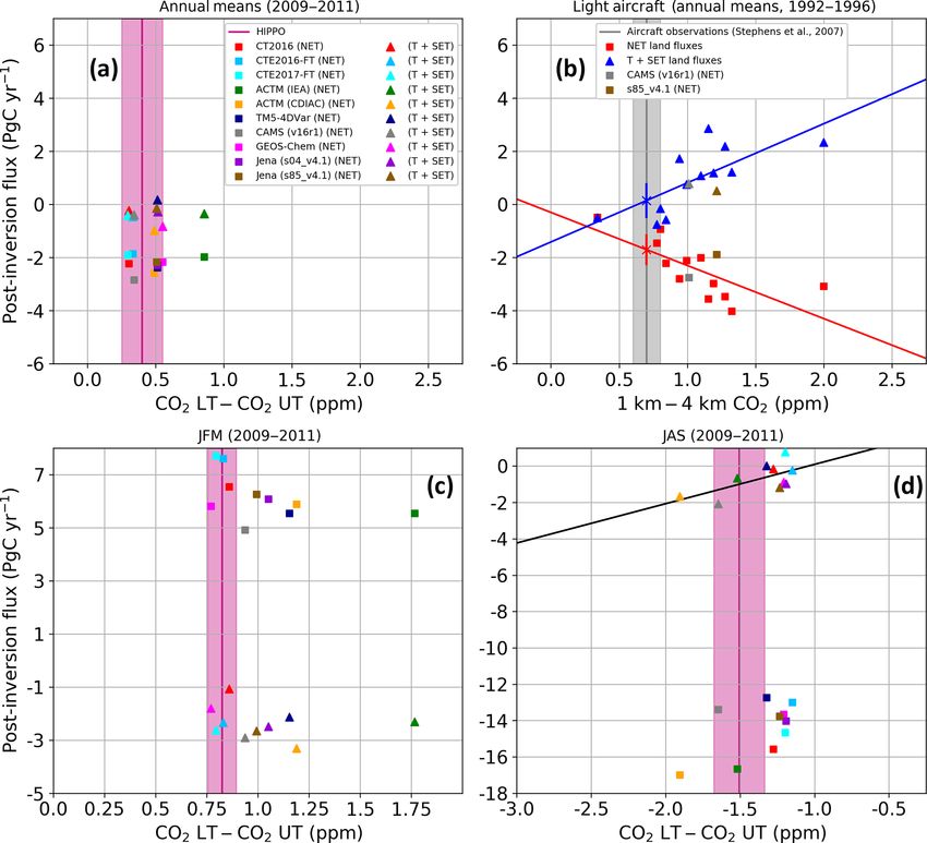
120                               B. Gaubert et al.: Drivers of remaining differences between converging global CO2 inverse models

Table 1. List of the inverse modeling systems used in this study and general characteristics.

      Acronym                References                                    Grid                 Fossil fuel                 Transport          Number of          Meteorological          Available
                                                                           spacing              priors                      model           vertical layers       fields                  period
      CAMS (v16r1)           Chevallier et al. (2005, 2010)a               3.75◦                CDIAC/GCP2016               LMDZ                           39     ERA-Interim             1979 to 2016
                                                                           ×1.875◦
      Jena (s04_v4.1)        Rödenbeck et al. (2003)                       4◦ × 5◦              CDIAC                       TM3                            19     NCEP                    2004 to 2016
                             Rödenbeck (2005)
      Jena (s85_v4.1)        –                                             4◦ × 5◦              CDIAC                       TM3                            19     NCEP                    2004 to 2016
      CTE2016-FT             van der Laan-Luijkx et al. (2017)             1◦ × 1◦              CDIAC                       TM5                            25     ERA-Interim             2001 to 2015
      CTE2017-FT             –                                             1◦ × 1◦              CDIAC                       TM5                            25     ERA-Interim             2000 to 2016
      CT2016                 Peters et al. (2007)b                         1◦ × 1◦              ODIAC v2016                 TM5                            25     NCEP                    2001 to 2015
                                                                                                and “Miller”
      ACTM-IEA               Saeki and Patra (2017)                        Inversion            IEA                         ACTM                           32     NCEP2                   2003 to 2011
                             Patra et al. (2011)                           (2.8◦ × 2.8◦ )                                                                         (for inversion)
      ACTM-CDIAC             –                                             and forward          CDIAC                       ACTM                           32     JRA25                   2003 to 2011
                                                                           (1.1◦ × 1.1◦ )                                                                         for forward
      TM5-4DVar              Basu et al. (2013)                            3◦ × 2◦              EDGAR                       TM5                            25     ERA-Interim             2007 to 2012
                                                                                                +CDIAC
      GEOS-Chem              Deng et al. (2014)                            4◦ × 5◦              CDIAC, ICOADS               GEOS                           47     GEOS5                   2009 to 2011
                                                                                                and 3-D aviation
   a With updates documented at https://atmosphere.copernicus.eu/ (last access: 7 January 2019). b With updates documented at https://carbontracker.noaa.gov (last access: 7 January 2019).

mentary interannual variability calculated from satellite data                                              clude observations over North America conducted between
when available (van der Werf et al., 2010; Giglio et al.,                                                   Colorado and Alaska (Fig. S1 in the Supplement). HIPPO
2013). The average ELUC for the year 2009 to 2011 included                                                  flew three different in situ CO2 instruments and two whole
here is estimated to be 0.85 PgC yr−1 with an uncertainty of                                                air samplers with laboratory CO2 measurements. We use the
0.5 PgC yr−1 . These emissions are added to the GCP2016                                                     recommended CO2.X variable which comes primarily from
land sink for comparison to atmospheric inversion estimates.                                                the Harvard quantum cascade laser spectrometer (QCLS),
   Finally, the land sink is estimated in GCP2016 as a resid-                                               gap filled during calibration sequences, and compare to the
ual from all other components of the carbon budget. The                                                     other systems to constrain potential systematic biases (see
GCP2016 method treats the riverine flux of carbon from land                                                 Supplement). We calculate the NET vertical gradient as the
to ocean to atmosphere as separate components of the total                                                  difference between the average from 1000 to 800 hPa for the
air–land and air–sea fluxes and subtracts an estimate of this                                               lower troposphere (LT) and the average from 800 to 400 hPa
flux (0.45 PgC yr−1 ; Jacobson et al., 2007) from the pCO2-                                                 for the upper troposphere (UT), spanning the latitude range
based sea-to-air flux estimates to match estimates of the an-                                               from 20 to 90◦ N. To do this, we first detrend the observa-
thropogenic ocean sink alone. Because the land sink is a                                                    tions and model sampled along the flight-track output by
residual, this increase in the magnitude of the ocean sink re-                                              subtracting a deseasonalized and smoothed long-term trend
sults in a corresponding reduction by 0.45 PgC yr−1 in the                                                  record from the fit of the Mauna Loa Observatory in situ
magnitude of the land sink in GCP2016. To compare to at-                                                    measurement time series to provide a common reference for
mospheric inverse flux estimates, which represent the total                                                 both observations and models, and we bin the observations
air–sea and air–land fluxes, we have adjusted the GCP2016                                                   by 100 hPa in pressure and 5◦ in latitude bins. We then fit
ocean and land flux estimates by this same 0.45 PgC yr−1 ,                                                  each bin with a curve using two harmonics and constant
decreasing the ocean sink and increasing the land sink.                                                     offset, and we average the resulting fits across boxes and
   Note that we do not show GCP2016 estimates here as a                                                     pressure levels, with latitude weighting (see Supplement).
truth metric against which to evaluate the models, but rather                                               Figure 1 shows the resulting daily fit of the annual cycle
as one estimate of an internally consistent global budget that                                              for the HIPPO observations and model simulations of the
provides a useful reference for exploring axes of variability                                               NET vertical gradient. Qualitatively, it shows that most mod-
in our models and comparing to other community estimates.                                                   els reproduce the CO2 cycle well, with positive gradients in
                                                                                                            winter over a broad peak and negative gradients in summer
2.3     HIPPO observations and fitting procedures                                                           over a narrower trough. The three CarbonTracker inversions
                                                                                                            (CT2016, CTE2016-FT, and CTE2017-FT) have somewhat
The HIPPO project (Wofsy, 2011) used the NSF/NCAR                                                           lower seasonal gradient amplitude, while the two ACTM in-
Gulfstream V aircraft (GV) to conduct 5-month-long cam-                                                     versions (ACTM-IEA and ACTM-CDIAC) show larger am-
paigns in different seasons over 3 years (2009–2011; see                                                    plitude. More quantitative details are given in Sect. 3.1. To
Supplement) that consisted of vertical profiling along North–                                               illustrate the temporal coverage of the observations, we plot
South-Pacific transects between 87◦ N and 67◦ S. The five                                                   the measurements of the nine HIPPO transects in Fig. 1 as
campaigns included nine transects of the NET Pacific. We ex-

Biogeosciences, 16, 117–134, 2019                                                                                                               www.biogeosciences.net/16/117/2019/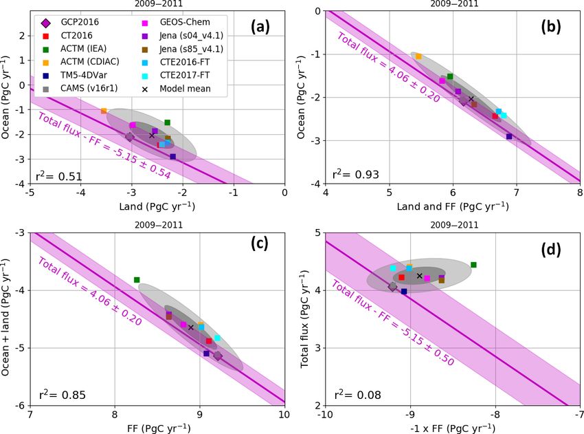
B. Gaubert et al.: Drivers of remaining differences between converging global CO2 inverse models                                         121

Figure 1. Reconstructed annual cycle in northern extratropical vertical CO2 gradients, obtained from fits using two harmonics of the HIPPO
data and correspondingly sampled model outputs, averaged over 20 to 90◦ N (1000 to 800 hPa minus 800 to 400 hPa). The CO2 average
curtain observations for each of nine atmospheric transects have been added on the graph to illustrate the data uncertainties and temporal
coverage, the y-axis error bar is derived from the range of disagreement among the three in situ instruments on board (QCLS, OMS, and
AO2; see Supplement), and the line average is derived from the CO2.X merged dataset. The horizontal whiskers represent the time span of
the flights contributing to each average. The observed line shown here is not a direct fit to the observation points, but rather comes from an
average of fits to individual 100 hPa by 5◦ latitude bins as described in the text.

simple differences of the latitude-weighted average concen-              S6). Also, because the models are driven by reanalysis winds,
trations within the LT and UT boxes for each transect, while             they should capture the position of synoptic systems and as-
an example of a fit to an individual bin is shown in Fig. S1.            sociated transport. However, the wind fields and model trans-
   The QCLS instrument has a 1σ precision of 20 ppb (San-                port may be biased, which could result in different vertical
toni et al., 2014), and for all five CO2 systems on the GV the           gradients for reasons unrelated to the fluxes of interest. We
instrumental precision is negligible for the large-scale aver-           have estimated synoptic variability in the vertical gradient
age metrics we present here. More relevant sources of uncer-             metric and find a worst-case potential model synoptic sam-
tainty are associated with the potential for altitude-dependent          pling bias of ±0.06 ppm for the annual mean, ±0.14 ppm for
biases that might result from inlet or cabin-pressure effects,           JFM, and ±0.15 ppm for JAS (1σ ; see Supplement).
as well as misrepresentation of synoptic transport in the mod-
els. We estimate (i) uncertainty in the annual-mean NET ver-
tical gradient metric by comparison of the five independent
instruments and whole air samplers to be ± 0.15 ppm (see                 3     Results
Supplement) and (ii) uncertainty on the individual HIPPO
transect values to range from 0.02 to 0.48 ppm as shown by               3.1    Fluxes and posterior CO2 comparisons with
the vertical bars in Fig. 1. These values are derived from the                  HIPPO
maximum absolute differences between the sensors, which
we conservatively treat as best-guess 1σ uncertainty esti-               Each individual inversion system adjusts fluxes to fit the con-
mates. These uncertainty estimates correspond to the vertical            centration fields with its given transport scheme and a pri-
gradient as observed by the HIPPO flight tracks and calcu-               ori source and sink information. Biases can appear in the re-
lated with the fitting procedure used here. Because we use               trieved posterior CO2 resulting from errors in the estimated
model output along the flight tracks and treat model output              fluxes or from specific biases in transport to the location of
and observations identically in our calculations, we do not              the independent data (here in particular vertical transport to
include an estimate of potential spatial sampling bias, but we           the upper atmosphere). We first evaluate if the spread of re-
do use model output to assess the spatial representativeness             trieved land fluxes over different zonal bands is correlated
of our calculated metrics with respect to full 150◦ W transect           with NET vertical CO2 gradients and if the modeled gradi-
and full zonal means in Sect. 4 of the Supplement (Figs. S5,             ents match observations, as was previously done for the T3L2
                                                                         models by Stephens et al. (2007).

www.biogeosciences.net/16/117/2019/                                                                  Biogeosciences, 16, 117–134, 2019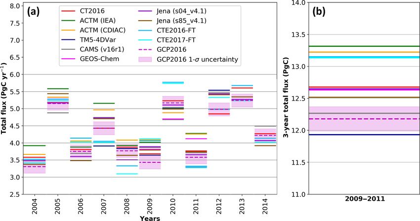
122                   B. Gaubert et al.: Drivers of remaining differences between converging global CO2 inverse models

    Figure 2a presents the results for the HIPPO and model         to a significant improvement in meteorological analyses and
vertical gradients and model fluxes, broken into NET and           forecasts (e.g., Healy, 2008).
T+SET regions for the years 2009–2011. The mean and                   One concern is the spatial representativeness of the HIPPO
relative spread of 10 simulations for the posterior annual         measurements which were made over the Pacific Ocean
mean NET land flux is −2.24 PgC yr−1 ±0.29 PgC yr−1                while the light-aircraft observations used by Stephens et al.
(13 %, 1σ ). Aside from the ACTM-IEA simulation, all mod-          (2007) were mostly measuring profiles over land. We discuss
els are within the uncertainty range of 0.15 ppm or 50 %           this issue in the Supplement and show that across models
of the measured vertical gradient. This contrasts to the           HIPPO vertical gradients are significantly representative of
TransCom 3 Level 2 simulations which had an annual mean            the zonal mean for the 3-year mean and every year individu-
of −2.42 PgC yr−1 ± 1.05 (43 %) PgC yr−1 for NET land              ally (Fig. S5). Seasonally (Fig. S6), it appears that the vertical
flux and disagreed with the observed vertical gradient by          gradients are representative of the parallel 150W for winter
∼ 0.5 ppm on average and as much as 1.3 ppm (186 %).               (JFM), spring (AMJ), and fall (OND) seasons, representa-
As listed in Table 1, the inversions have significant differ-      tive of the zonal mean for winter (JFM) and fall (OND), and
ences in transport model, resolution, and driving meteorol-        representative of the zonal average over land only in boreal
ogy and are converging despite these differences. In addition,     summer (JAS). We did find a significant correlation between
there are no apparent relationships between vertical gradi-        vertical gradients defined by the HIPPO flight tracks and land
ents and NET nor T+SET land fluxes. The standard devi-             zonal means during summer (JAS), when vertical gradients
ation across 10 simulations on the difference between NET          are weak.
land and T+SET is 0.4 PgC yr−1 while it was 2.1 PgC yr−1 in           Figure 2c and d show the vertical gradients and fluxes for
T3L2 (Gurney et al., 2004; Gurney and Denning, 2013) and           2009–2011 winter (JFM) and summer (JAS). The agreement
1.28 PgC yr−1 in RECCAP (Peylin et al., 2013), representing        between the models and HIPPO observations is not as strong
a steady and dramatic convergence of model estimates over          as for annual means. The vertical gradient in the NET winter
the past 15 years. We reproduce the Stephens et al. (2007)         is reasonably well reproduced by nine models with differ-
annual mean figure in Fig. 2b, with the exception of show-         ences lower than 0.36 ppm. The ACTM-IEA inversion is an
ing T+SET instead of T, to highlight those differences. It is      outlier and overestimates by 0.94 ppm the winter season av-
important to note that these results correspond to a different     erage vertical gradient. For ACTM, the global annual IEA
period and different models, with a smaller network of as-         emissions are less than CDIAC (Fig. 4c and d), which re-
similated in situ network measurements and assimilation of         sults in a weaker northern extratropical sink (Figs. 2s and 3a)
monthly mean rather than discrete measurements. We took            that corresponds with a more positive LT–UT northern extra-
advantage of the two models that span the 1992–1996 pe-            tropical gradient (Figs. 2a and S2) and a more positive N–S
riod, CAMS (v16r1) and Jena (s85_v4.1), to further inves-          gradient (Fig. S2), comparing just the two ACTM versions.
tigate differences from the T3L2 period. Those two models          Differences across inversion systems in Fig. S2 also depend
are quite close to the 2009–2011 vertical gradient observa-        on the transport and inversion scheme and the resulting spa-
tions (Fig. 2a), but they both overestimate the 1992–1996          tial distribution of sources and sinks.
vertical gradients (Fig. 2b). Notably, they fall along the lines      There are generally larger differences between observed
fit to the T3L2 models in Fig. 2b, which could be a coinci-        and modeled vertical gradients in Northern Hemisphere sum-
dence, but might also suggest that despite agreeing with the       mer (JAS), with only two models (ACTM-IEA and CAMS)
other models on the latitudinal flux distribution for 2009–        within observation error bars, but the whole range of val-
2011 these models overestimate tropical sources and north-         ues is only 0.75 ppm. In this case a linear relationship (r 2 =
ern sinks during 1992–1996. This would require that these          0.4) is found between the modeled vertical gradient and the
models be more dependent on vertical mixing biases in the          retrieved T+SET fluxes, but not for the NET flux. There
earlier period. The different number of assimilated sites is       is a significant relationship between HIPPO and the land-
one potential factor that might explain different biases in re-    only zonal average vertical gradient and both are corre-
trieved fluxes for these two periods, but this is not seen for     lated with the T+SET fluxes (Fig. S7), but with a slope of
the comparison of the two versions of the Jena model as-           2.16 ppm yr PgC1 for HIPPO while it is 0.93 ppm yr PgC1
similating different numbers of sites during 2009–2011. It is      over land where the vertical gradients are bigger. This sug-
worth noting that reanalyses of meteorological observations        gests that transport errors may be more critical in the summer
have noticeably improved thanks to a better representation         season or that other factors compensate to obscure the rela-
of unresolved processes in global models, improved data as-        tionship for these relatively coarse time averages in other sea-
similation methods, and the increasing availability of satel-      sons and for the annual means. While additional insights into
lite data, which makes the reanalyses perform better in the        model behavior could be gained from more detailed compar-
2000s than for the 1990s and earlier (e.g., Gelaro et al., 2017;   isons to individual models or in more controlled inversion en-
Bauer et al., 2015). As an example, the assimilation of new        sembles, the varied nature of these inversion systems makes
observations from the constellation of COSMIC global posi-         detailed analyses more challenging and beyond the scope of
tioning system radio occultation (GPSRO) satellites has led        our current study.

Biogeosciences, 16, 117–134, 2019                                                         www.biogeosciences.net/16/117/2019/
B. Gaubert et al.: Drivers of remaining differences between converging global CO2 inverse models 123
For the annual means and winter there are no statistical re- and s04_v4.1 for 2009–2011 is rather small (Fig. 3a), less
lationships between the vertical gradients and the retrieved than 0.15 PgC yr−1 .
fluxes. This suggests that Northern Hemisphere vertical mix- According to GCP2016, the total land sink in 2009–2011
ing errors do not play a major role in biasing the flux estima- was around twice as large (around 3 PgC yr−1 ) compared to
tion across these models. However, the retrieved fluxes can that for 1992–1996 (around 1.7 PgC yr−1 ) and 2001–2004
still be biased because of the transport errors. (around 1.3 PgC yr−1 ). This is due to the combined effect of
One potential limitation in our analysis could be the use of natural interannual variability as well as a long-term trend
similar meteorological fields from the ECMWF base analy- (Ballantyne et al., 2012). The retrieved total land fluxes for
sis and forecast cycle, which is the case for 5 out of 10 sim- all study periods appear to be close to the corresponding GCP
ulations. A careful comparison of model transport suggests estimates with most models falling within the GCP2016 1σ
that nudging to a particular reanalysis product does not imply uncertainty range. For the 2001–2004 period, the newer sim-
identical tracer transport between the models (e.g., Prather ulations move fluxes parallel to the GCP line in the direction
et al., 2008; Locatelli et al., 2015; Orbe et al., 2017). The of a weaker tropical source and a weaker NET sink relative
transport errors arise from resolved advection and heav- to the original RECCAP estimates. For the 1992–1996 pe-
ily parameterized transport schemes such as convection and riod, one of the two newer simulations shifts fluxes in that
boundary layer mixing (Locatelli et al., 2015; Orbe et al., same direction, but not as far as suggested by Stephens et al.
2017; Krol et al., 2018). Qualitatively, we cannot distinguish (2007).
the CO2 vertical gradient from models using ERA-Interim However, we have revisited the Stephens et al. (2007) es-
winds from the five other models. timates, by considering the intercept of the regression lines
with the aircraft observations rather than the mean of the
3.2 The latitudinal distribution of retrieved land fluxes three models nearest the annual mean observations and eval-
uating the error using the standard error of the linear regres-
In this section, we present the retrieved land flux partitioning sions. The selection of three models by Stephens et al. (2007)
between the NET and the T+SET, as shown in Fig. 3 and Ta- was somewhat arbitrary as they did not directly overlap the
ble 2. Because the total sink is the sum of T+SET and NET, observations and did not agree as well as other models sea-
these lines have a slope of −1 and any deviation perpendic- sonally. This new approach relying on the correlated signal
ular to the lines indicates disagreement on the total land sink from all models leads to a NET flux of −1.7±0.59 PgC yr−1
from the GCP2016 estimate. As noted in the previous sec- and a T+SET flux of 0.15 ± 0.66 PgC yr−1 , a similar shift in
tion, inverse modeling results for the HIPPO period (2009– NET fluxes but only two-thirds of the shift in T+SET fluxes
2011) are remarkably close to one another (Fig. 3a). These using the Stephens et al. (2007) subset of models, as shown
results converge on a NET land sink value slightly larger in Fig. 3b.
than 2 PgC yr−1 (−2.24 ± 0.29 PgC yr−1 ) and a T+SET land For the RECCAP period, we used their Group 1 sim-
sink of−0.38 ± 0.31 PgC yr−1 . In Fig. 3, multi-model means ulations (JENA, LSCE, MACC-II, CT2011_oi, CTE2013)
are represented by blue diamonds and associated error bars identified in Peylin et al. (2013), four of which assimi-
are estimated by the standard deviation across models. The lated the observations at the sample time as opposed to us-
2009–2011 period is marked by a large tropical land sink be- ing monthly means and all of which solved for fluxes at
cause of the strong La Niña event of 2011 (Bastos et al., the resolution of the transport model or for small ecore-
2013; Poulter et al., 2014). For these 3 years, the models gions over land. The T+SET flux estimate averaged over the
clearly indicate a negative flux over the tropics and SET land. RECCAP Group 1 models is 0.34 ± 0.27 PgC yr−1 . This is
There are also increasing lines of evidence that the rate of nearly identical to the average of the new models from this
deforestation and climate stress over tropics have been mod- study (0.34 ± 0.27 PgC yr−1 ; using CTE2016-FT, CTE2017-
erated in recent decades (e.g., 2000s), compared to the 1990s FT, CT2016, CAMS v16r1, and Jena s85_v4.1). Both es-
(Kondo et al., 2018), with a reduced change in tropical for- timate slightly positive T+SET fluxes that are only half of
est cover because the decrease in the South American defor- the RECCAP all-model average (0.93 ± 0.90 PgC yr−1 ). Our
estation has been compensated for by an increased Southeast NET land sink estimates using newer models are less than the
Asian deforestation (Hansen et al., 2013). previous estimates in the original T3L2 and RECCAP stud-
In order to place these recent flux estimates in the con- ies for the 1992–1996 and 2001–2004 periods. Conversely,
text of previous studies, we show the flux estimates by the our new estimates suggest a change in the T+SET flux to-
new models that also estimate fluxes for the earlier peri- wards greater uptake and/or less emission for these periods;
ods; two models have available outputs for the T3L2 pe- we found a decrease in the T+SET land flux by 0.71 PgC yr−1
riod (1992–1996) and four for the RECCAP period (2001– from 0.56 ± 0.32 PgC yr−1 for the 1994–2004 period com-
2004), as shown in Fig. 3b and c. For Jena, one inversion pared to −0.15 ± 0.43 PgC yr−1 for the 2004–2014 period
(s85_v4.1) starts in 1985 and is constrained by only 23 at- (Fig. S9). Then, to obtain a flux estimate less sensitive to
mospheric sites while the other (s04_v4.1) starts in 2004 and year-to-year variability we calculate the fluxes for the full
uses 59 sites. Interestingly, the difference between s85_v4.1 11-year 2004–2014 period (Fig. 3d), for which we have five
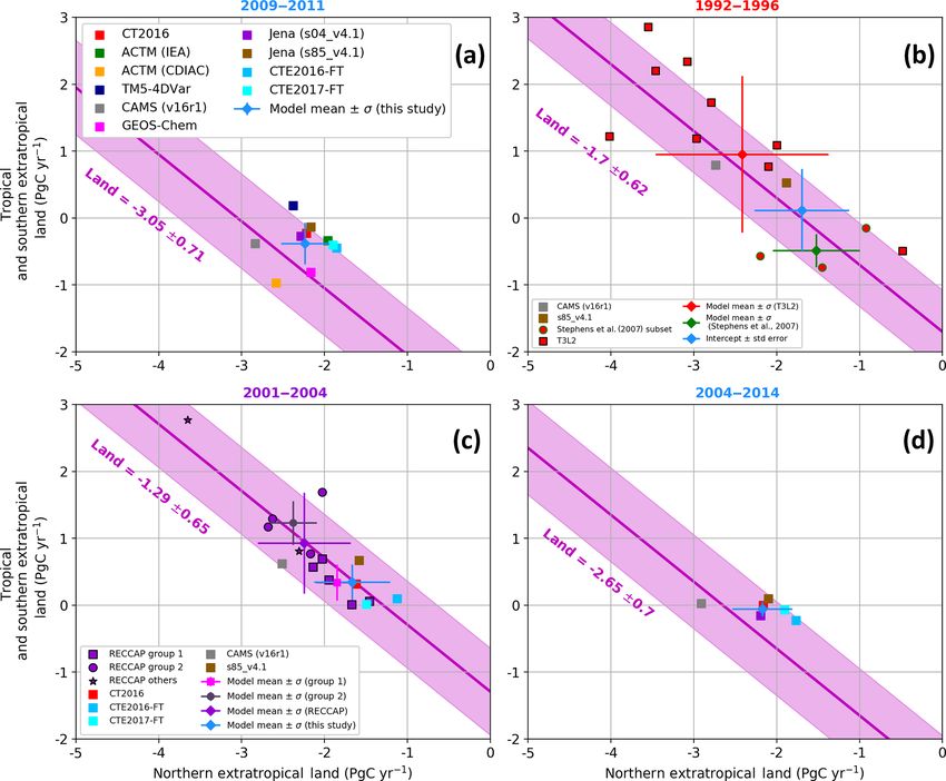
www.biogeosciences.net/16/117/2019/ Biogeosciences, 16, 117–134, 2019124 B. Gaubert et al.: Drivers of remaining differences between converging global CO2 inverse models Figure 2. Retrieved fluxes versus NET vertical gradients. (a) Annual mean NET land and T+SET land fluxes versus posterior NET vertical gradients (lower minus upper troposphere) from model output along HIPPO flight tracks and HIPPO observations (pink line) for the period 2009–2011. The shaded area represents an estimate of measurement uncertainty of ±0.15 ppm for the annual mean, as estimated in the Sect. S2 in the Supplement. Inverse model posterior concentration gradients and fluxes are shown as points (squares represent NET; triangles represent T+SET). The vertical axis represents the integrated annual mean land fluxes (PgC yr−1 ). (b) Same as (a) but for 1992–1996 and showing TransCom 3 Level 2 models and our two current models that span this time period, showing dependence of posterior fluxes on transport and a large range of transport biases. Annual mean NET (red squares) and T+SET (blue triangles) land carbon fluxes for 1992– 1996 estimated by the 12 T3L2 models plotted as a function of the models’ post-inversion predicted mean vertical CO2 gradients at 10 light-aircraft profiling sites (adapted from Stephens et al., 2007) with fluxes partitioned by TransCom region. The Jena (s85_v4.1) and the CAMS (v16r1) simulations have also been sampled at the same light-aircraft locations but their fluxes are partitioned at 20◦ N and 20◦ S. The crosses show our new best estimate of the fluxes estimated by the regression of all T3L2 models. The error bars on these points are estimated using the standard error of the regressions. (c) Same as panel (a) for January–February–March (JFM), and (d) same as panel (a) for July–August–September (JAS). For the seasonal plots, the width of the pink bar is 0.07 ppm for JFM and 0.17 for JAS. In panel (d), the black line represents the regression line, shown because the relationship is statistically significant at a 95 % confidence interval. model estimates. For this longer period, the model spread is 3.3 Variation in retrieved global carbon budgets largely reduced, in particular for the NET land fluxes, and again we find near-neutral T+SET land fluxes. Taking all four The global carbon budget partitioning for 2009–2011 is of the estimation periods together (Table 2) all of our central shown for our suite of models and for GCP2016 (river ad- estimates for T+SET are within 0.4 PgC yr−1 of zero. The justed) in Fig. 4 with the model mean and GCP2016 reported tropical land fluxes are −0.2 ± 0.3 PgC yr−1 for 2009–2011 in Table . In every panel of Fig. 4, the light-pink error band and 0.0 ± 0.12 PgC yr−1 for 2004–2014. This implies a con- shows the constraint imposed by fixing the values to those of sistent uptake of carbon by intact tropical forests over several GCP2016, and the associated equation is shown on the graph. decades. The pink diamond represents the GCP2016 estimate while Biogeosciences, 16, 117–134, 2019 www.biogeosciences.net/16/117/2019/
B. Gaubert et al.: Drivers of remaining differences between converging global CO2 inverse models                                         125

Figure 3. Tropical and southern extratropical (T+SET) versus northern extratropical (NET) land fluxes for the periods (a) 2009–2011,
(b) 1992–1996, (c) 2001–2004, and (d) 2004–2014. The new models used in this study are represented by squares and the average of the
available or selected simulations is shown in blue with 1 standard deviation error bars. The pink line and shaded area represents the GCP2016
(river adjusted) estimates of the total land sink for the given period. (a) Results for the HIPPO period 2009–2011; (b) results for the T3L2
period 1992–1996. The TransCom 3 Level 2 outputs (Gurney et al., 2004) are shown in red, with the vertical gradient selected models from
Stephens et al. (2007) as circles outlined in green and the rest as red squares outlined in black. The intercept of the regression line with
the observed vertical gradient (Fig. 2) is used to define our best flux estimate with error bars estimated by the standard error of the linear
regression. (c) Results for the RECCAP period 2001–2004. Also, from Peylin et al. (2013), model means and standard deviations are shown
in pink for the subgroup 1 (Jena, LSCEa, MACC-II, CTE2013, CT2011_oi) and in gray for the subgroup 2 (MATCH, CCAM, TrC, NICAM).
Panel (d) shows the results from our new set of models for the period 2004–2014.

the cross and the gray shaded area show the model mean and               the GCP2016 estimates in Fig. 4, the two are independent,
1 standard deviation in darker and 2 standard deviations in              except for the FF and for the atmospheric data that serve to
lighter gray. For the models, the total flux is calculated as            estimate the total flux in GCP2016. By mass balance, the to-
the subtraction of the ocean and land sink from the FF emis-             tal annual flux must equal the total growth rate integrated
sions. Note that by mass conservation the total flux equals              over the entire atmosphere, and this is what we refer to as the
the whole-atmosphere growth rate (WAGR), but that WAGR                   total flux.
may differ from the MBL atmosphere growth rate (AGR) de-                    The integrated ocean versus land fluxes are presented
fined by surface stations, because of sampling biases or in-             in Fig. 4a. The equation for the range of ocean and land
terannual variability in tropospheric mixing or stratosphere–            fluxes that would match FF and the total flux estimates
troposphere exchange. GCP uses the MBL AGR (Dlugo-                       from GCP2016 is also shown in Fig. 4a. The models and
kencky and Tans, 2018) as an estimate of total flux and as-              GCP2016 agree well on the ocean flux with a mean of
signs uncertainty of ±0.19 PgC yr−1 (Le Quéré et al., 2016)              −2.04 ± 0.51 PgC yr−1 over the 3 years of 2009–2011. The
for recent decades, with speculation that the relative uncer-            multi-model mean of the land flux is −2.61 ± 0.42 PgC yr−1 .
tainty should decrease when averaging multiple years. Note               The GCP2016 land flux is −3.04 ± 0.5 PgC yr−1 and thus
that, even though the CAMS results systematically align with             overestimates the model mean. The cloud of model ocean

www.biogeosciences.net/16/117/2019/                                                                  Biogeosciences, 16, 117–134, 2019
126                      B. Gaubert et al.: Drivers of remaining differences between converging global CO2 inverse models

Table 2. Previous and our new best estimates (in bold) of the latitudinal partitioning of land fluxes over four time periods. All values are in
PgC yr−1 . Values are indicated by the model mean ± 1 standard deviation or 1σ error uncertainties. Regarding the T3L2 period (Gurney
et al., 2004), our new estimate for the 1992–1996 period comes from the intercept of the fit lines with the observations in Fig. 2b, and the
uncertainties on these values come from the standard error on these metrics from the fits. Regarding the RECCAP period (Peylin et al., 2013),
our new estimate for the 2001–2004 period is the average of the five new models from this study.

                        Time period     Source                    Number of models           NET land       T+SET land
                        1992–1996       T3L2                                       12    −2.42 ± 1.05      0.95 ± 1.17
                                        Stephens et al. (2007)                      3    −1.52 ± 0.53     −0.49 ± 0.25
                                        T3L2 (intercept)                           12    −1.70 ± 0.59      0.15 ± 0.66
                        2001–2004
                                        RECCAP all models                          11    −2.25 ± 0.58       0.93 ± 0.90
                                        RECCAP Group 1                              5    −1.85 ± 0.25       0.34 ± 0.27
                                        This study                                  5    −1.67 ± 0.46       0.34 ± 0.27
                        2009–2011
                                        This study                                 10    −2.24 ± 0.29     −0.38 ± 0.31
                        2004–2014
                                        This study                                  6    −2.17 ± 0.36     −0.05 ± 0.11

Figure 4. Synthesis of globally integrated fluxes for the 2009–2011 period, in PgC yr−1 . Each inversion is represented by a square and the
model mean by a × symbol. The GCP2016 estimates are a pink diamond, which is sometimes hard to see because it is superimposed in each
panel by the gray CAMS point. We have adjusted the GCP2016 ocean and land flux estimates by the riverine flux of carbon from land to
ocean to atmosphere (0.45 PgC yr−1 ; Jacobson et al., 2007; Le Quéré et al., 2018), decreasing the ocean sink and increasing the land sink.
The magenta line and light-pink shaded area show the corresponding mass balance estimates from GCP2016. In each panel the line and
equation shown represent the sum of the x and y variables, and thus the line has a slope of −1, and any deviation perpendicular to the line
indicates disagreement on the sum. Here we use the total flux which by mass balance is the whole-atmosphere growth rate (see text), and
for panels (a) and (d), the total flux – FF line also equals O + L, while for panels (b) and (c), the total flux line equals O + L + FF. Ellipses
denote the variability around the model means of 1σ (darker gray) and 2σ (lighter gray). (a) Ocean versus land; (b) ocean versus land + FF;
(c) ocean + land versus FF; (d) total flux versus −1× FF.

Biogeosciences, 16, 117–134, 2019                                                                  www.biogeosciences.net/16/117/2019/
B. Gaubert et al.: Drivers of remaining differences between converging global CO2 inverse models 127
Table 3. Global Carbon budget for 2009 to 2011, estimated by the certainty prescribed to them or, more specifically, the range
Global Carbon Project 2016 (first row, with river adjustment) and of FF estimates used by leading inversions exceeds the un-
by the suite of models from this study (second row); all values are certainty that GCP2016 places on the CDIAC estimates.
in PgC yr−1 . Values are indicated by the model mean ±1σ error This implies that uncertainties in FF emissions do not ade-
uncertainties, provided by GCP2016 or by the model standard devi- quately consider potential regional biases (Peylin et al., 2011;
ation.
Thompson et al., 2016; Saeki and Patra, 2017). The large
FF Land Ocean Total flux spread of model results along the mass balance line in 4C
GCP2016 9.21 ± 0.46 −3.04 ± 0.50 −2.05 ± 0.50 4.06 ± 0.20
highlights the need (i) to reduce uncertainty in estimates of
Multi-model 8.9 ± 0.29 −2.61 ± 0.42 −2.04 ± 0.51 4.25 ± 0.14 FF emissions and (ii) to develop modeling systems that re-
lax rigid FF prior constraints and observational systems that
can support optimizing FF emission estimates. For the period
1980–2015, the total flux estimates from GCP2016 are esti-
versus land flux estimates are rather scattered around the mated by the MBL AGR of Dlugokencky and Tans (2018).
model mean with a correlation coefficient of only 0.51. Only background sites that are located in the MBL are used
To better understand the reasons for these discrepancies, in this calculation. Ballantyne et al. (2012) calculated a sam-
and specifically to investigate how much of the land spread pling error of 0.38 PgC yr−1 (2σ ) among the 40 sites and a
in Fig. 4a is a result of differences in fossil fuel priors, we GCP2017 estimate uncertainty of ±0.19 PgC yr−1 (1σ ) for
plotted the ocean flux versus the sum of land and FF emis- the period 1980–2015 with respect to the total flux. We show
sions in Fig. 4b. This figure shows a tight correlation across the model-retrieved WAGR (equal to total flux) for each in-
models for these two parameters (r 2 = 0.93). Given that prior dividual year in Fig. 5 along with the GCP2016 estimate
uncertainties specified in the inversions for ocean fluxes are and error bars. The total spread in the total flux from the
typically smaller than those for land and fossil emissions are inverse models over the 3 years of 2009–2011 equates to
fixed, this implies, for a given ocean and FF flux combina- 1.38 PgC as shown in Fig. 5b. This is well outside of the
tion, the models are adjusting the land fluxes while matching uncertainty range estimated for the extrapolation of MBL
CO2 observations. While combining land and fossil fluxes measurements, implying several inversions are not rigidly
together reduces the random scatter, it does not reduce the constrained to match observed MBL AGR, even over peri-
range of the continental fluxes, illustrating the fact that mod- ods of 3 years. Because CO2 is variably mixed in different
els do not simply compensate for biases in fossil priors years and by different models in the troposphere and between
with land fluxes, but rather that ocean fluxes are affected the troposphere and the stratosphere, some inconsistency be-
too (Saeki and Patra, 2017). Conversely, we plot the sum of tween the MBL-defined AGR and the total flux of CO2 in
ocean and land fluxes against FF emissions in Fig. 4c. This the models might be expected. However, using CT2017 as
figure shows that the ocean + land total sink is largely con- a test case, the annual difference between the model total
trolled by the prescribed FF emissions. In general, the mod- surface flux and the observed MBL growth rate over 2000–
els use smaller fossil fuel sources than reported in GCP2016. 2016 has a standard deviation of 0.29 PgC yr−1 and for 3-
Figure 4d compares the opposite of FF emissions versus the year averages within this period a standard deviation of only
total flux, again defined by subtraction of the land and ocean 0.10 PgC yr−1 , which is much smaller than the discrepancies
fluxes from FF. The spread in models is not parallel to the shown in Fig. 5. Buchwitz et al. (2018) made a similar AGR
line defined by the GCP2016 budget closure. We hypothe- comparison using CAMS output of total column and surface
size that models that overestimate fossil emissions prioritize data and also found good agreement with differences of only
matching the spatial distribution of CO2 and thus estimate ±0.2 PgC yr−1 (1σ ) on an annual basis. Another potential
overcompensating sinks. The spatial patterns of the different challenge to inversions having a consistent total flux during
FF priors must also play a role, as well as the strength of the this time may be due to large interannual variability in nat-
atmospheric constraint on annual timescales imposed by the ural fluxes, with rapid changes resulting from different cli-
inversion systems. matic conditions from the moderate El Niño of 2009 to the
Taking the two extreme models the ACTM-CDIAC and strong La Niña of 2011 (Bastos et al., 2013; Poulter et al.,
TM5-4DVar estimates provide very different distributions of 2014). This period has also been marked by rapid changes
fluxes. ACTM-CDIAC suggests stronger land sinks, both in emissions, related to lower emissions in 2009 during the
over the NET and the T+SET regions, and a lower ocean financial crisis and a rapid increase in 2010 (Peters et al.,
sink while TM5-4DVar suggests the opposite. This leads to 2011). However, Fig. 5 does not indicate that the model to-
a range of around 2 PgC yr−1 on the model ocean sink. Be- tal flux estimates for the years 2009–2011 are more divergent
cause of an intentionally different FF source, but with the than other years. Further work investigating these differences
same inversion system, the ACTM-CDIAC and ACTM-IEA is needed but is beyond the scope of this study. In particular,
retrieved land fluxes differ by slightly less than 1 PgC yr−1 the length of the assimilation window may have an impact. It
and ocean fluxes differ by 0.5 PgC yr−1 . Overall, this anal- may also be possible to force the inverse systems to agree, at
ysis suggests that errors in FF priors are larger than the un-
www.biogeosciences.net/16/117/2019/ Biogeosciences, 16, 117–134, 2019128 B. Gaubert et al.: Drivers of remaining differences between converging global CO2 inverse models
least within the MBL, with the observationally defined AGR, 4. For the 1992–1996 period, we define an update to the
and this may help to reduce model spread elsewhere. Stephens et al. (2007) result, using the intercept of the
model output linear regression with the observed an-
nual mean vertical gradient of 0.7 ppm, leading to a
4 Summary and future work NET land uptake of −1.7±0.57 PgC yr−1 and a T+SET
flux of 0.12±0.62 PgC yr−1 for 1992–1996. Our results
Atmospheric transport has long been a major contributor to for the more recent decadal period, the 11 years from
top-down atmospheric inverse model flux uncertainty. We ap- 2004 to 2014, indicate a somewhat larger NET sink of
plied the technique of Stephens et al. (2007) to a suite of 2.21 ± 0.34 PgC yr−1 and a neutral tropical land flux of
state-of-the-art inversion systems assimilating primarily sur- 0.04 ± 0.13 PgC yr−1 , in line with a trend of a larger
face observations to take advantage of the unique HIPPO land sink (Sarmiento et al., 2010; Keenan et al., 2016)
global airborne dataset for independent validation in assess- if shared across both latitudinal bands.
ing fluxes. We also compared the models to each other and
5. We present our best estimates of the latitudinal land
to the GCP2016 carbon budget synthesis. The major findings
flux partitioning for the four periods 1992–1996, 2001–
of these comparisons can be summarized as follows:
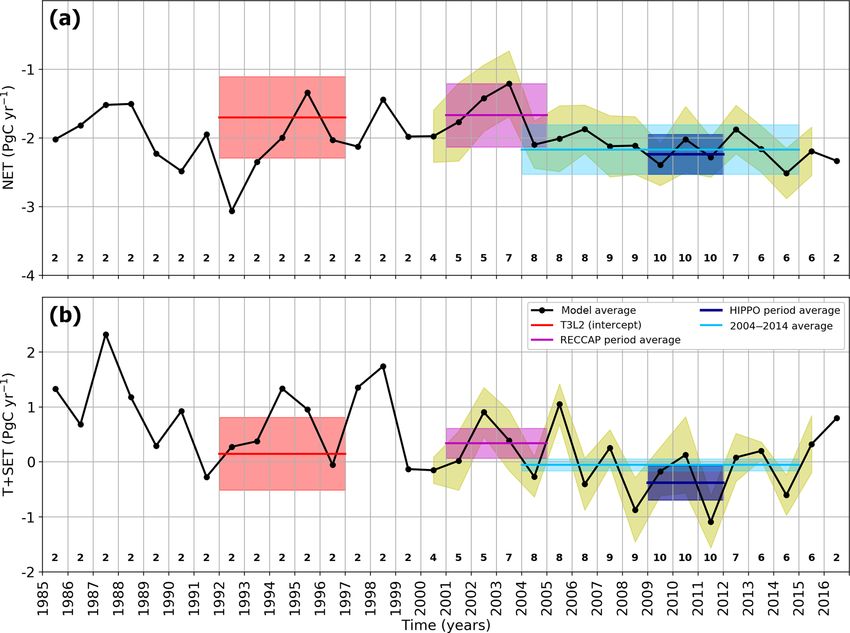
2004, 2009–2011, and 2004–2014 in Table 2. We
1. Model estimates of the latitudinal distribution of present in Fig. 6 the time series of the NET and T+SET
land fluxes are remarkably consistent across mod- land fluxes from 1979 to 2016, using all simulations
els and this represents a convergence over the past available in this study. This figure shows a decrease in
15 years of inverse model development. The stan- the T+SET land flux by 0.71 PgC yr−1 , from +0.56 to
dard deviation across our 10 simulations of the differ- −0.15 PgC yr−1 between the decades 1994–2004 and
ence between northern extratropical land and tropical 2004–2014, respectively. The land-use change flux es-
land fluxes is 0.4 PgC yr−1 for the period 2009–2011 timated by GCP2017 was nearly identical for these two
and 0.43 PgC yr−1 for the period 2004–2014 across time periods (+1.31 and +1.29 PgC yr−1 , respectively),
five models. These are considerable reductions from and assuming these numbers primarily reflect tropical
2.1 PgC yr−1 for 12 simulations in T3L2 (differing only land-use change emissions this implies an increase in
in transport modeling) for the period 1992–1996 and the intact tropical forest sink on decadal timescales.
1.28 PgC yr−1 for 11 simulations in the RECCAP study Our re-evaluations of the T3L2 and RECCAP study re-
for the period 2001–2004. sults (Table 2) confirm that the sum of the tropics and
southern extratropics have been near neutral for several
2. Our suite of 10 inversions gives a NET land uptake decades, despite large-scale tropical deforestation, and
of −2.22 ± 0.27 PgC yr−1 (1σ ) and a net T+SET up- in accordance with the recent literature on the tropical
take of −0.37 ± 0.31 PgC yr−1 for 2009–2011 (−0.2 ± land carbon budget (Hansen et al., 2013; Keenan et al.,
0.3 PgC yr−1 for the tropics only). For 2004–2014, 2016; Mitchard, 2018).
a subset of six models gives NET land uptake of 6. At the global scale, we find in agreement with earlier
−2.17 ± 0.36 PgC yr−1 , T+SET uptake of −0.06 ± studies that our model results are strongly dependent on
0.11 PgC yr−1 , and T of 0.0 ± 0.12 PgC yr−1 , thus al- the prescribed FF emissions. While the total of global
lowing for deforestation implying a strong uptake in in- land and ocean uptake adjusts to match differences in
tact tropical forests, in line with forest inventories (Pan FF emissions, this compensation is not perfect.
et al., 2011).
7. Our suite of 10 simulations also retrieve surprisingly
3. The group of RECCAP models that primarily assim- different 3-year whole atmospheric growth rates, as de-
ilated discrete rather than monthly mean observations fined by the total fluxes. The model range is 1.38 PgC
agrees with estimates from our subset of five newer over 3 years, compared to an estimated uncertainty of
models regarding the lack of strong net emissions from ±0.10 PgC in CT2017 matching between MBL CO2
tropical land. This is not too surprising because most concentration trends and total flux over 3 years and a
of our models, with the exception of LSCEa, are the 0.2 PgC yr−1 uncertainty assigned by GCP2017. The
updated versions of the same models in the RECCAP yearly ranges of up to 1 PgC yr−1 in the model total
Group 1 (Peylin et al., 2013). Those five models esti- flux estimates imply 0.5 ppm disagreements in whole-
mated a net NET land sink of −1.85 ± 0.25 PgC yr−1 atmosphere CO2 concentrations, and the 1.4 PgC yr−1
and our subset of four models covering the REC- range for the 3-year period implies disagreements of
CAP period estimate of −1.71 ± 0.5 PgC yr−1 . Regard- 0.7 ppm in the whole-atmosphere CO2 concentration
ing T+SET, the newer model estimate is a source of change over that time period.
0.34 ± 0.27 PgC yr−1 , while it is 0.34 ± 0.27 PgC yr−1 Across seven state-of-the-art systems running 10 inver-
in RECCAP’s Group 1. sions, there does not appear to be a correlation between pos-
Biogeosciences, 16, 117–134, 2019 www.biogeosciences.net/16/117/2019/You can also read