HARMONISING PLANT FUNCTIONAL TYPE DISTRIBUTIONS FOR EVALUATING EARTH SYSTEM MODELS - MPG.PURE
←
→
Page content transcription
If your browser does not render page correctly, please read the page content below
Clim. Past, 15, 335–366, 2019
https://doi.org/10.5194/cp-15-335-2019
© Author(s) 2019. This work is distributed under
the Creative Commons Attribution 4.0 License.

Harmonising plant functional type distributions for
evaluating Earth system models
Anne Dallmeyer1 , Martin Claussen1,2 , and Victor Brovkin1
1 MaxPlanck Institute for Meteorology, Bundesstrasse 53, 20146 Hamburg, Germany
2 MeteorologicalInstitute, Centrum für Erdsystemforschung und Nachhaltigkeit (CEN), Universität Hamburg,
Bundesstrasse 55, 20146 Hamburg, Germany

Correspondence: Anne Dallmeyer (anne.dallmeyer@mpimet.mpg.de)

Received: 28 March 2018 – Discussion started: 6 April 2018
Revised: 4 December 2018 – Accepted: 24 January 2019 – Published: 18 February 2019

Abstract. Dynamic vegetation models simulate global veg-         However, as the new method considers the PFT distributions
etation in terms of fractional coverage of a few plant func-     actually calculated by the Earth system models, it allows for
tional types (PFTs). Although these models often share the       a direct comparison and evaluation of simulated vegetation
same concept, they differ with respect to the number and kind    distributions which the classical method cannot do. Thereby,
of PFTs, complicating the comparability of simulated vege-       the new method provides a powerful tool for the evaluation
tation distributions. Pollen-based vegetation reconstructions    of Earth system models in general.
are initially only available in the form of time series of in-
dividual taxa that are not distinguished in the models. Thus,
to evaluate simulated vegetation distributions, the modelling    1   Introduction
results and pollen-based vegetation reconstructions have to
be converted into a comparable format. The classical ap-         Within dynamic global vegetation models (DGVMs), the nat-
proach is the method of biomisation, but hitherto PFT-based      ural vegetation distribution is usually represented in the form
biomisation methods were only available for individual mod-      of plant functional types (PFTs); i.e. plants are grouped with
els. We introduce and evaluate a simple, universally appli-      regard to their physiology and physiognomy (Prentice et al.,
cable technique to harmonise PFT distributions by assign-        2007). These PFTs differ with respect to phenology, albedo,
ing them into nine mega-biomes, using only assumptions on        morphological and photosynthetic parameters and are usu-
the minimum PFT cover fractions and few bioclimatic con-         ally constrained by an individual bioclimatic range of tol-
straints (based on the 2 m temperature). These constraints       erance defined by temperature thresholds. These thresholds
mainly follow the limitation rules used in the classical biome   represent the cold resistance, chilling and heat requirements
models (here BIOME4). We test the method for six state-          of the plants and determine the area where the PFTs can be
of-the-art dynamic vegetation models that are included in        established.
Earth system models based on pre-industrial, mid-Holocene           In most DGVMs, a “mosaic” approach is used; i.e. each
and Last Glacial Maximum simulations. The method works           grid box of the land surface is split into separate parts for
well, independent of the spatial resolution or the complex-      a non-vegetated and a vegetated fraction that is further tiled
ity of the models. Large biome belts (such as tropical for-      in mosaics, taking subgrid-scale heterogeneity into account.
est) are generally better represented than regionally confined   Thus, several PFTs can cover the same grid cell and compete
biomes (warm–temperate forest, savanna). The comparison          for space via their net primary productivity (e.g. Sitch et al.,
with biome distributions inferred via the classical biomisa-     2003; Krinner et al., 2005; Reick et al., 2013). Non-vegetated
tion approach of forcing biome models (here BIOME1) with         area (seasonally bare soil or permanently bare ground) is pro-
the simulated climate states shows that the PFT-based biomi-     duced where plant productivity is too low.
sation is even able to keep up with the classical method.

Published by Copernicus Publications on behalf of the European Geosciences Union.
336                                                           A. Dallmeyer et al.: Harmonising plant functional type distributions

   Although the main principles for the calculation of PFT            both simulated by LPJ. With this method, reconstructed ma-
distributions are similar among most DGVMs, they vary re-             jor biome shifts could be reproduced. Roche et al. (2007)
garding the number and kind of PFTs used to represent the             used the dominant PFT and the bioclimate limits defined in
global vegetation. Natural (non-anthropogenic) PFTs range             the biome model BIOME1 (Prentice et al., 1992) to biomise
from 2 in, e.g. VECODE (for definition of the acronyms of             PFT cover fractions for the Last Glacial Maximum (LGM)
the DGVMs, see Table 1), to 10 in, e.g. LPJ and ORCHIDEE              simulated by VECODE. As VECODE distinguishes as main
(Table 1). Even within the same model, PFT variety can dif-           PFTs only trees and herbaceous plants, not all biome types
fer between individual simulations, e.g. due to the inclusion         defined in BIOME1 could be considered (e.g. no shrubs).
of land-use types. These differences among the simulations            The computed biome map shows reasonable agreement with
and models prohibit the intermodel comparability of simu-             LGM land cover reconstructions. A similar approach was
lated global vegetation distributions and the comparability           chosen by Handiani et al. (2012, 2013) for calculating biome
with pollen-based biome reconstructions.                              distributions during Heinrich event 1, based on PFT sim-
   Pollen records are originally displayed in the form of             ulations of TRIFFID and CLM-DGVM. As these models
pollen percentages or pollen accumulation rates, what cannot          strongly deviate in their PFT classification, they applied dif-
be directly compared to plant functional type distributions, as       ferent methods for biomisation. For TRIFFID, they first cal-
pollen records do not reflect the actual plant abundances. For        culated the dominant PFT in each grid cell following the
a systematic comparison of simulated plant functional type            method by Crucifix et al. (2005) and afterwards used tem-
distributions and reconstructions, both need to be converted          perature limitation defined in BIOME4 (Kaplan et al., 2003)
in a compatible format. In the last two decades, taxa to PFT          to assign the dominant PFTs to mega-biomes. For CLM-
assignment methods and the method of “biomisation” for                DGVM, potential dominant PFTs were estimated by adopt-
pollen-based reconstructions have been developed (e.g. Pren-          ing the scheme of Schurgers et al. (2006) and biomes were
tice et al., 1996; Ni et al., 2010; Harrison et al., 2010), so that   differentiated with the help of temperature limitations that
pollen assemblages can be grouped into biomes (e.g. tropical          follow the environmental constraints defined in CCSM3 (i.e.
forest, temperate steppe, desert). Pollen-based biome synthe-         the fully coupled model used in their study, including the
ses have been provided (Prentice et al., 1998, 2000; Bigelow          land and vegetation model CLM-DGVM).
et al., 2003; Ni et al., 2010; Harrison, 2017; Tian et al., 2017)        Recently, Prentice et al. (2011) introduced another ap-
that have extensively been used to evaluate simulated biome           proach of biomising plant functional type distributions sim-
distributions obtained from diagnostic biome models such as           ulated by dynamic vegetation models. In their method, sim-
BIOME1 or BIOME4 (e.g. Prentice et al., 1992; Haxeltine               ulated foliage projective cover (FPC) is used to distinguish
and Prentice, 1996; Kaplan et al., 2003). These biome mod-            between desert, grassland/dry shrubland and forest biomes,
els can be forced by observed or simulated climate fields and         which are further divided into forest and savanna-like biomes
calculate biome distributions in equilibrium to this input cli-       through the vegetation height. The assignment to, e.g. bo-
mate. Using this classical method of biomisation, fundamen-           real, temperate or tropical forest/savanna (or parkland) is
tal palaeo-vegetation analysis can be undertaken (e.g. Jolly          controlled by the tree-PFT composition. Climate limits are
et al., 1998; Harrison et al., 2003, 2016; Wohlfahrt et al.,          only used to distinguish the tundra biome. This method has
2008; Dallmeyer et al., 2017) without requiring an explicit           successfully been used in several palaeo-vegetation studies
calculated vegetation distribution by the Earth system models         (Kageyama et al., 2013; Calvo and Prentice, 2015) using dif-
(ESMs). On the other hand, this also means that existing sim-         ferent versions of the LPJ and ORCHIDEE models.
ulated plant functional type distributions calculated by the             All of these methods have in common that they have been
DGVMs being dynamically coupled in these models are ne-               designed for individual models and hence need specific out-
glected, since only the simulated climate pattern is taken into       put not necessarily provided by all models. Therefore, these
account. The biomisation via diagnostic biome models did              methods cannot directly be adopted for all existing dynamic
not include any information on the original PFT distribution          vegetation models. A consistent intermodel comparison of
simulated by the Earth system models. As the DGVMs are                the simulated vegetation distribution and an evaluation of the
generally more complex than the biome models and include              models against reconstructions on biome level is so far not
more relevant processes, valuable information included in the         possible.
PFT distribution gets lost in the classical biomisation by the           To harmonise (palaeo)-vegetation distributions simulated
biome models. A more appropriate method of biomisation                by dynamic vegetation models and thereby facilitate the eval-
would be to directly use the PFT distributions calculated by          uation of Earth system models (ESMs) and the comparison
the DGVMs.                                                            of model results and biome reconstructions, we developed a
   Several model studies have taken up this problem by in-            biomisation technique that is based on the PFT distributions
troducing methods for biomising PFT distributions simulated           simulated by DGVMs, few input variables and simple differ-
by DGVMs. Schurgers et al. (2006) derive biome maps for               entiation rules. These include bioclimatic constraints using
the Eemian and mid-Holocene from the relative fractional              near-surface air temperature and assumptions on maximum
coverage of the individual PFTs and the soil temperature,             required PFT coverage. The aim of developing this method

Clim. Past, 15, 335–366, 2019                                                                    www.clim-past.net/15/335/2019/
A. Dallmeyer et al.: Harmonising plant functional type distributions                                                                 337

Table 1. The PFTs used in the different state-of-the-art dynamic global vegetation models. These are the Jena Scheme for Biosphere Atmo-
sphere Coupling in Hamburg (JSBACH), the Lund–Potsdam–Jena model (LPJ), the Organising Carbon and Hydrology In Dynamic Ecosys-
tems model (ORCHIDEE), the Community Land Model’s dynamic global vegetation model (CLM-DGVM), the Top-down Representation
of Interactive Foliage and Flora Including Dynamics (TRIFFID) model and the Vegetation Continuous Description model (VECODE).

  PFT class       JSBACH                     LPJ              ORCHIDEE          CLM-DGVM         TRIFFID                   VECODE
  Tropical        tropical                   tropical         tropical          tropical         broadleaf trees and         trees
  trees           broadleaf                  broadleaf        broadleaf         broadleaf        needleleaf trees
                  evergreen                  evergreen        evergreen         evergreen
                  tropical                   tropical         tropical          tropical
                  broadleaf                  broadleaf        broadleaf         broadleaf
                  raingreen                  raingreen        raingreen         raingreen
  Extratropical   extratropical              temperate        temperate         temperate
  trees           evergreen                  needleleaf       needleleaf        needleleaf
                                             evergreen        evergreen         evergreen
                                             temperate        temperate         temperate
                                             broadleaf        broadleaf         broadleaf
                                             evergreen        evergreen         evergreen
                                             boreal           boreal            boreal
                                             needleleaf       needleleaf        needleleaf
                                             evergreen        evergreen         evergreen
                  extratropical              temperate        temperate         temperate
                  deciduous                  broadleaf        broadleaf         broadleaf
                                             deciduous        deciduous         deciduous
                                             boreal           boreal            boreal
                                             needleleaf       needleleaf        deciduous
                                             deciduous        deciduous
                                             boreal           boreal
                                             broadleaf        broadleaf
                                             deciduous        deciduous
  Shrubs          raingreen                                                                      shrubs
                  shrubs
                  cold
                  deciduous
                  shrubs
  Grass           C3 grass                   C3 grass         C3 grass          Arctic grass     C3 grass                 herbaceous
                                                                                C3 grass
                  C4 grass                   C4 grass         C4 grass          C4 grass         C4 grass

was not to construct a better biomisation method than the             2     Methods
classical method via diagnostic biome models but to develop
a more direct method that can convert PFT distributions into          2.1    Biomisation
biomes so that the additional information included due to the
coupling of the DGVM will not get lost.                               The PFT cover fractions simulated by the individual dynamic
   We test this method on pre-industrial, mid-Holocene and            vegetation models are converted into nine different mega-
Last Glacial Maximum vegetation simulations performed in              biomes (Fig. 1), using few bioclimatic limits and assump-
nearly all state-of-the-art dynamic vegetation models. The            tions on the maximum required coverage of certain PFTs.
skill of this biomisation approach is quantified via (standard)       The aggregation into the mega-biomes is in line with the def-
metrics, by comparing the converted biome maps with esti-             initions of the BIOME6000 project (cf. Harrison, 2017) that
mates of modern potential biome distributions (Ramankutty             are also commonly used for grouping pollen-based biome re-
and Foley, 1999) and pollen-based biome reconstructions               constructions. Bioclimatic limits and the differentiation rules
(Biome6000 database, Harrison, 2017).                                 basically follow the biome assignment of the BIOME4 model
                                                                      (Kaplan et al., 2003). As input data, only climatological

www.clim-past.net/15/335/2019/                                                                       Clim. Past, 15, 335–366, 2019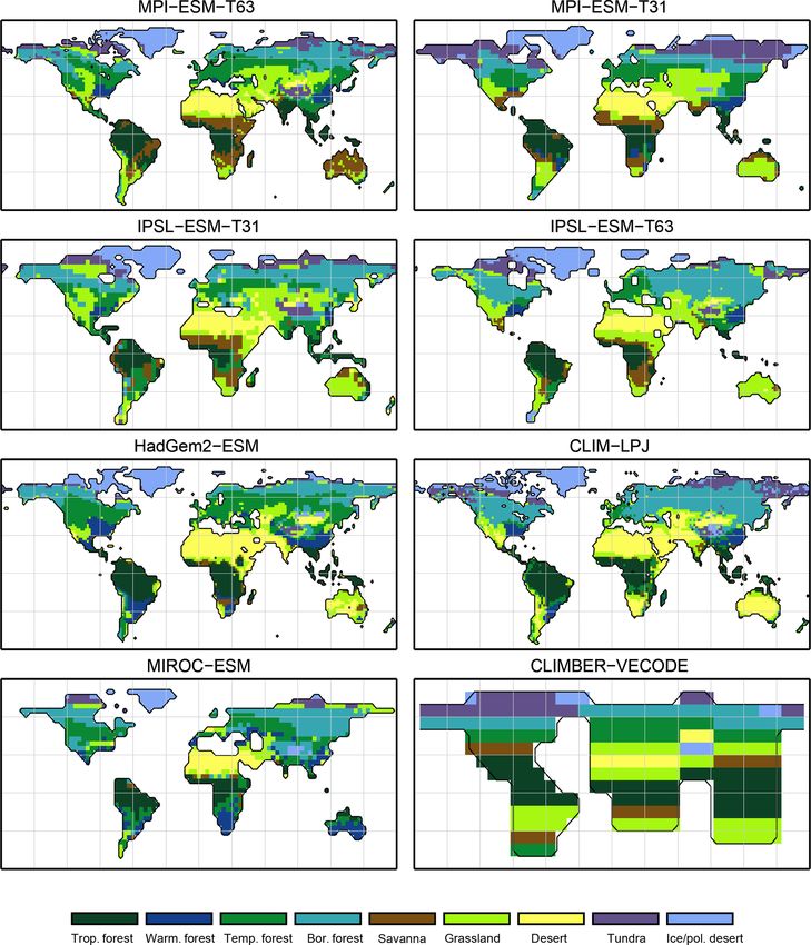
338 A. Dallmeyer et al.: Harmonising plant functional type distributions
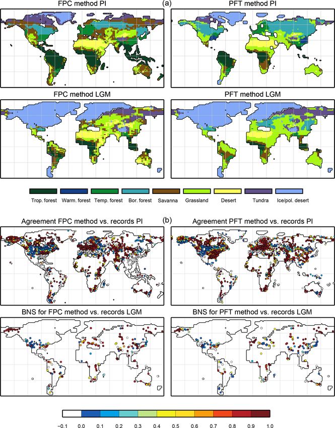
Figure 1. Scheme of the biomisation method. The PFT fractions simulated by the individual DGVMs are assigned to the PFT groups “desert”
(i.e. 1 minus total vegetation), “grass” (containing all grass PFT types) “woody PFT” (containing all trees and shrub types) and “trees”
(containing all tree types). The “trees” and “woody PFTs” are further differentiated into “tropical trees”, “temperate trees”, “temperate
woody PFTs” and “boreal woody PFTs” via bioclimatic limitations (Table 2). For DGVMs explicitly distinguishing tropical, temperate
or boreal tree types, the original classification of the DGVM is used. Afterwards, the PFT groups are assigned to nine mega-biomes by
assumptions on the minimum coverage of certain PFT groups needed in a grid cell and additional bioclimatic limitations (Table 2).
mean growing degree days (GDD0 and GDD5), monthly For the biomisation, the forests are considered first; i.e. re-
mean 2 m air temperature and multi-year mean PFT cover gions in which trees or woody PFTs are dominant or cover an
fractions (e.g. averaged over 100 years) are required. The area more than 25 % are assigned to tropical, temperate and
limitation to few climatic rules and few variables needed en- boreal forests according to the PFT groups. From the tem-
ables the application of the method to all state-of-the-art dy- perate forest, warm regions (i.e. GDD5 > 3000 ◦ C) revealing
namic vegetation models. a dominant temperate tree fraction are subtracted and as-
In detail, the PFTs calculated by the respective dynamic signed to the biome “warm–temperate forest”. The remaining
vegetation models are aggregated into the groups “trees”, area is then tested for fulfilling the constraints for the non-
“woody PFTs” (i.e. shrubs and all tree PFTs), “grass” and forest biomes. First, the savanna and dry woodland region
“desert”, which is calculated as 1 minus the total vegeta- is identified by bioclimatic limitations (GDD5 > 1200 and
tion. If the model includes land-use types, the affected ar- Tc > 10 ◦ C) and a woody PFT coverage of at least 25 %. The
eas are redistributed to the other PFTs by simply scaling up remaining vegetated area is assigned to the biome “grass-
the other PFT fractions proportionally to their ratio of the to- land and dry shrublands”, if GDD0 exceeds 800 ◦ C, or to
tal natural vegetation. Based on these groups, regions domi- the biome “tundra”, if GDD0 is below 800 ◦ C (cf. BIOME4;
nated by trees and regions in which the cover fraction of the Kaplan et al., 2003). The non-vegetated area, i.e. regions in
woody PFTs exceeds 25 % (with the additional constraint of which the total vegetation cover is less than 20 %, is either
the total vegetation cover exceeding 50 %) are identified, as assigned to warm or to cold desert, depending on whether
these are necessary conditions for the assignment of the land the annual mean temperature is above or below 2 ◦ C. For
cover to forest biomes. Afterwards, the groups “trees” and the biome “tundra”, only 10 % vegetation cover is needed. A
“woody PFTs” are split into boreal (GDD5 ≤ 900 ◦ C), tem- flow chart summarising the details of the PFT-based biomi-
perate (GDD5 > 900 ◦ C) and tropical trees or woody PFTs sation is shown for the VECODE model in Appendix A.
(Tc > 15.5 ◦ C) via temperature limits (cf. Table 2). If any of We are aware of the simplicity of this approach, calculat-
these tree PFTs are simulated directly in the vegetation model ing the tundra and the grassland and dry shrubland biomes
(e.g. in LPJ or ORCHIDEE), the original distributions are as a residual of the non-forested area, not directly depending
taken and the PFT group is assigned to the dominant tree on the simulated grass PFT fraction. We decided to attribute
type, i.e. the tree type that covers the largest fraction of the the main priority to the forested biomes as this is also the
grid cell. These PFT groups (i.e. boreal woody PFTs, temper- strategy commonly used in DGVMs and biome models.
ate trees and woody PFTs, tropical trees, grass and desert) are To assess the performance of the biomisation based on
the first consistent vegetation classification shared by all in- simulated PFTs, we additionally biomise the simulated cli-
put simulations, so that model-to-model comparison is also mate fields corresponding to the PFT distributions in each
possible on this PFT level. model. This is the conventionally used procedure to biomise
general circulation model (GCM) or ESM output (further re-
Clim. Past, 15, 335–366, 2019 www.clim-past.net/15/335/2019/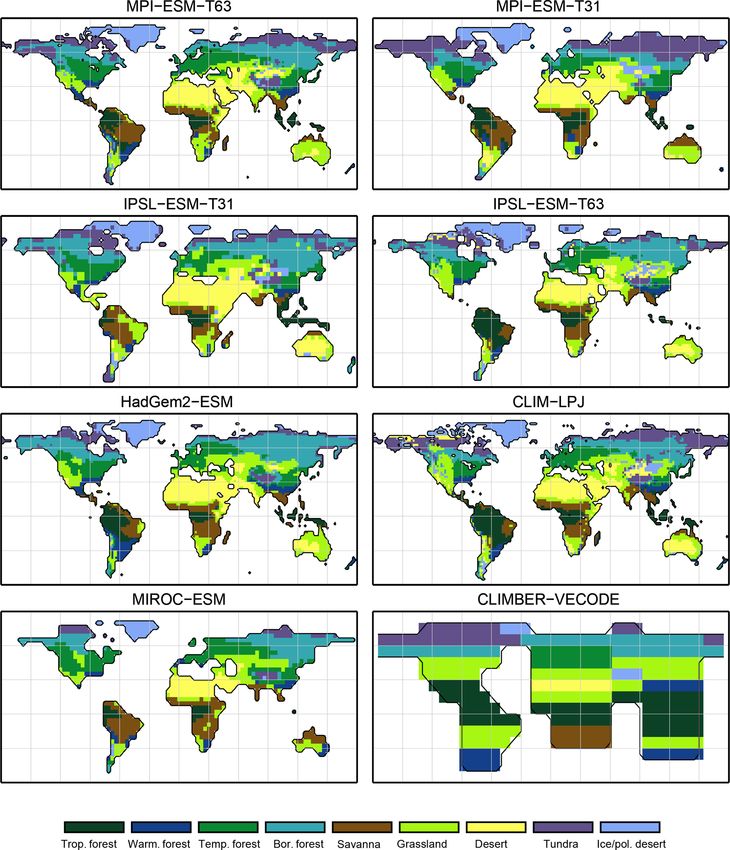
A. Dallmeyer et al.: Harmonising plant functional type distributions                                                                    339

Table 2. Bioclimatic limits and assumptions on minimum PFT coverage needed for the assignment of PFTs into the PFT groups and into the
nine mega-biomes. The separation of boreal, temperate and tropical tree PFTs is based on the same bioclimatic limits as the respective forest
mega-biomes. Only temperature-based limitations are used, i.e. the growing degree days on a basis of 5 ◦ C (GDD5) or on a basis of 0 ◦ C
(GDD0), the monthly mean temperature of the coldest month (Tc) and the annual mean temperature (Tann ). Bioclimatic limits are mainly
taken from the BIOME4 model (Kaplan et al., 2003, marked with ∗ ). The limit for tropical forest is taken from BIOME1 (Prentice et al.,
1992) but is also commonly used in DGVMs (e.g. JSBACH). The limit for the differentiation of deserts has been empirically determined in
this study and is close to the value chosen by Handiani et al. (2013) and within the range of the Köppen–Geiger climate classification for
polar climate and the Holdridge alpine life zone classification. The Tc limit for warm savannas is taken from JSBACH (C4 grass criteria)
to exclude temperate savannas. The assumptions on minimum coverage have been partly taken, partly empirically adapted from Handiani
et al. (2013). A flow chart displaying the biomisation procedure is shown in Appendix A for the VECODE model, the DGVM used in the
CLIMate-BiosphERe 2 (CLIMBER-2) model.

                 Mega-biome                            Minimum coverage needed               Bioclimatic limitations
                 Tropical forest                       Tropical trees dominant               Tc > 15.5 ◦ C
                 Warm–temperate forest                 Temperate trees dominant              GDD5 > 3000 ◦ C∗
                 Temperate forest                      Temperate woody PFTs dominant         900 ◦ C < GDD5 ≤ 3000 ◦ C∗
                 Boreal forest                         Boreal woody PFTs dominant            GDD5 ≤ 900 ◦ C∗
                 (Warm) savanna and dry woodland       Woody PFT coverage > 0.25             GDD5 > 1200 ◦ C∗ , Tc > 10 ◦ C
                 Grassland and dry shrubland           Total vegetation cover > 0.2          GDD0 ≥ 800 ◦ C∗
                 Tundra                                Total vegetation cover > 0.1          GDD0 < 800 ◦ C∗
                 (Warm) desert                         Total vegetation cover < 0.2          Tann > 2 ◦ C
                 Polar desert/ice                      Total vegetation cover < 0.2          Tann < 2 ◦ C

ferred to as the classical approach or climate-based method).            with fixed vegetation distribution, but this has essentially no
For this purpose, we use the biome model BIOME1 (Pren-                   effect on the biomisation procedure. Therefore, we include
tice et al., 1992) that calculates the biome distribution in             these simulations in our analysis. Nevertheless, the PFT-
equilibrium to the input climate. As forcing, BIOME1 needs               based biome distributions for these simulations are expected
the monthly mean climatological precipitation, near-surface              to fit better to the references than the other simulations that
temperature and cloudiness, which were taken from each                   ran with interactive vegetation.
simulation considered in this study, respectively. This clas-               We emphasise that this study is thought of as an introduc-
sical biomisation approach can only handle climate data as               tion and detailed evaluation of a new biomisation method. It
input; the simulated PFT distributions from the ESMs used in             is not seen as evaluation of the different vegetation models
the here-introduced PFT-based method are ignored. The orig-              with respect to the skill of simulating biome or vegetation
inal biomes have been grouped into the same mega-biome                   distributions. For this purpose, the different vegetation mod-
classification that is used for the PFT-based approach.                  els would have to be forced by the same climate state. Such
                                                                         an ensemble including all DGVMs (used here) does not ex-
2.2   Simulations                                                        ist. Therefore, we had to take individual simulations that all
                                                                         deviate with respect to the prescribed or simulated climate in
Simulations from nearly all state-of-the-art global dynamic              the coupled models. These differences in the climatic field
vegetation models that are included in Earth system mod-                 among the models and between the models and observations
els have been selected for biomisation. Six different models             (general climate biases) lead – per se – to differences in the
could be considered (i.e. JSBACH, TRIFFID, ORCHIDEE,                     simulated vegetation distributions and biases to the reference
SEIB, LPJ and VECODE). Overall, eight simulations for                    vegetation distribution.
the pre-industrial climate (PI) and vegetation, four for mid-
Holocene (6 ka) conditions and five for Last Glacial Max-
                                                                         2.3   Preparing the reference datasets
imum (LGM) conditions have been used (Table 3). Most
of these simulations were performed within CMIP5/PMIP3                   As reference, we use the estimated global potential natural
under strict simulation and output protocols enabling direct             vegetation map by Ramankutty and Foley (1999, referred to
comparison between the models (Braconnot et al., 2011;                   as RF99 in the following), which is a combination of mod-
Taylor et al., 2012). These include the models MPI-ESM-P,                ern satellite-based vegetation observations (i.e. the DISCover
IPSL-CM5A-LR, MIROC-ESM and HadGem2-ESM. Fur-                            land cover dataset) and the vegetation compilation prepared
ther details on the models and simulations are described in              by Haxeltine and Prentice (1996) that has been taken for re-
Appendix B.                                                              gions dominated by land use at present day. The RF99 dataset
   For the pre-industrial time slice, two out of eight simula-           is available at 5 min resolution and distinguishes 15 different
tions (MPI-ESM-T63 and IPSL-ESM-T31) were performed                      biome types that are similar to the mega-biome classification

www.clim-past.net/15/335/2019/                                                                           Clim. Past, 15, 335–366, 2019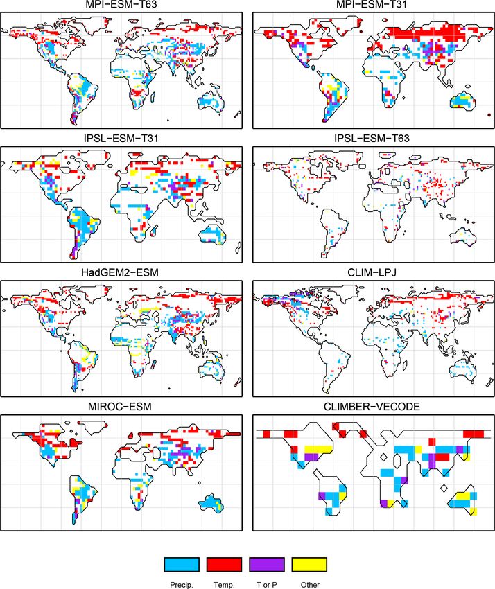
340                                                             A. Dallmeyer et al.: Harmonising plant functional type distributions

Table 3. Overview of the simulations used for testing the biomisation method. Listed are the model acronym, the model name, the name
of the included DGVM, the simulations used in this study, the spatial resolution used in the simulations, the number of PFTs (natural plus
anthropogenic) and the simulation reference. Simulations marked with the ∗ symbol include land use. Simulations marked with the # symbol
ran with prescribed vegetation.

 Model acronym       Model (DGVM)             Period      Resolution          PFT    Reference
 MPI-ESM-T63         MPI-ESM-P                PI∗ #       T63                8+4     cmip5.output1.MPI-M.MPI-ESM-P.piControl.mon.
                     (JSBACH)                                                        land.Lmon.r1i1p1.v20120315
                                              6 ka                                   cmip5.output1.MPI-M.MPI-ESM-P.midHolocene.
                                                                                     mon.land.Lmon.r1i1p2.v20120713
                                              LGM                                    cmip5.output1.MPI-M.MPI-ESM-P.lgm.mon.land.
                                                                                     Lmon.r1i1p2.v20120713
 MPI-ESM-T31         MPI-ESM-P                PI, LGM     T31                    8   Klockmann et al. (2016)
                     (JSBACH)                                                        (piCTL, LGMref)
 IPSL-ESM-T31        IPSL-CM5A-LR             PI∗ #       1.875◦ × 3.75◦    10 + 2   pmip3.output.IPSL.IPSL-CM5ALR.piControl.
                     (ORCHIDEE)                                                      monClim.land.Lclim.r1i1p1.v20140428
 IPSL-ESM-T63        CRUNCEP or               PI, LGM     2◦ × 2◦              10    Zhu (2016),
                     IPSL-CM5A-LR                                                    Zhu et al. (2018)
                     (ORCHIDEE-MICT)
 HadGEM2-ESM         HadGEM2-ES               PI∗         1.875◦ × 1.25◦     6+2     cmip5.output1.MOHC.HadGEM2-ES.piControl.
                     (TRIFFID)                                                       mon.land.Lmon.r1i1p1.v20111007
                                              6 ka                                   cmip5.output1.MOHC.HadGEM2-ES.midHolocene.
                                                                                     mon.land.Lmon.r1i1p1.v20120222
 CLIM-LPJ            CRU/CLIMBER-2            PI, 6 ka    0.5◦ × 0.5◦            9   Similar to Kleinen et al. (2010)
                     (LPJ)
 MIROC-ESM           MIROC-ESM                PI∗         T42                8+2     cmip5.output1.MIROC.MIROC-ESM.piControl.
                     (SEIB)                                                          mon.land.Lmon.r1i1p1.v20120710
                                                                                     Watanabe et al. (2011)
                                              6 ka                                   cmip5.output1.MIROC.MIROC-ESM.midHolocene.
                                                                                     mon.land.Lmon.r1i1p1.v20120710
                                              LGM                                    cmip5.output1.MIROC.MIROC-ESM.lgm.mon.
                                                                                     land.Lmon.r1i1p1.v20120710
 CLIMBER             CLIMBER-2                PI, LGM     10◦ × 10◦              2   Thomas Kleinen (personal communication, 2017)
                     (VECODE)

used here. Thus, most biomes could directly be assigned to              ues in the models. These differences in, e.g. atmospheric CO2
the mega-biome types (Table C1 in Appendix C). The prepa-               concentration between the reference datasets and the simula-
ration of the RF99 reference dataset is explained in more de-           tions may lead to small discrepancies in the model. In addi-
tail in Appendix C.                                                     tion, the references may be disturbed by anthropogenic influ-
   As further reference data, we use pollen-based biome                 ences.
reconstructions that are available for the modern, mid-                    Climatological monthly mean data of the years 1901–
Holocene and Last Glacial Maximum time slices within the                1930 from the University of East Anglia Climate Research
Biome6000 database (Harrison, 2017). The biome recon-                   Unit Time Series 4.00 (CRU TS4, University of East Anglia,
structions have been grouped into the mega-biomes accord-               2017) have been taken as the pre-industrial reference climate.
ing to the suggestions made by the Biome6000 project.                   This is the earliest period available. The CRU TS4 refer-
   Both vegetation datasets are derived for the modern time             ence climate has additionally been used as forcing for the
slice not exactly corresponding to the pre-industrial period            BIOME1 model to provide a best guess for the pre-industrial
(around 1850 AD) simulated in the models. While the ice                 biome map. We assume that neither the biomisation of simu-
sheet, the topography and the orbital conditions used for the           lated climate states (i.e. the classical method) nor the biomi-
pre-industrial control simulations are prescribed from mod-             sation of simulated PFTs can agree better with any refer-
ern conditions, greenhouse gases are set to pre-industrial val-         ence than this biome distribution, derived with a highly tuned

Clim. Past, 15, 335–366, 2019                                                                         www.clim-past.net/15/335/2019/
A. Dallmeyer et al.: Harmonising plant functional type distributions                                                                  341

biome model and the best global climate observation avail-                but may contain a large extra-regional component, depend-
able. Therefore, we use the level of agreement between the                ing, e.g. on the configuration (mainly the size) of the lake
CRU TS4 biome map and the RF99 or the Biome6000 recon-                    (Jacobsen and Bradshaw, 1981). A single grid-cell-to-point
structions as target value for our new biomisation method.                comparison is thus only partly meaningful; more advisable is
The reference biome distributions and the CRU TS4-based                   the inclusion of the surrounding grid cells of the sites. There-
biome map are displayed in Fig. 2.                                        fore, we looked for a metric taking agreement in the neigh-
                                                                          bourhood into account (such as the fuzzy kappa statistic) that
2.4     Metrics                                                           could easily be adapted to site to gridded-data comparison.
                                                                          We decided to use the fractional skill score (FSS; Roberts
2.4.1    Kappa statistic                                                  and Lean, 2008). While this method was initially developed
The kappa statistic (Cohen, 1960) is a widely used quantita-              and applied for expressing the performance of precipitation
tive map-comparison technique that has often been applied                 forecasts (e.g. Gilleland et al., 2009; Mittermaier et al., 2013;
for assessing the performance of vegetation simulations (e.g.             Wolff et al., 2014), it has recently been successfully used for
Monserud and Leemans, 1992; Prentice et al., 1992; Diffen-                different hydrological patterns (Koch et al., 2017). We fur-
baugh et al., 2003; Tang et al., 2009). The kappa statistic not           ther adapted the FSS method to biome distributions. For each
only includes the actual observed similarity (p0 ) of two cate-           mega-biome type, the reference (ref) and simulation (sim)
gorical maps but also considers the expected agreement (pe ),             are truncated into a binary map; i.e. we construct 18 maps
i.e. the agreement by chance. For each pair of compared grid              (9 for the reference, 9 for the simulation), in which the grid
cells (or a pair of grid cell and site) taken from the reference          cell being covered by the respective mega-biomes is filled
and the simulated biome distributions, a confusion matrix is              with the value “1” and all other grid cells are assigned to the
prepared containing all combinations of referenced and sim-               value “0”. Based on these maps, the mean fractional cover-
ulated biomes. Based on this error matrix, the agreement for              age of the respective mega-biome within the neighbourhood
each individual mega-biome is given by the following (Eq. 1,              Nij (three grid cells in each direction for T31, six for T63,
taken from Tang et al., 2009):                                            one for a 10◦ grid) of each cell is calculated for the reference
                                                                          and the simulation. Afterwards, the mean square error (MSE)
              pii − pi,r pc,i                                             between the simulation and the reference fractions for each
κi =                               ,                             (1)
         pi,r + pc,i /2 − pi,r pc,i                                       individual mega-biome is calculated and normalised by the
                                                                          MSE representing the worst-case agreement (MSEw), i.e. the
where pii is the individual entry for biome i on the main                 MSE reflecting no similarity between the reference and the
diagonal of the confusion matrix and pi,r and pc,i are the                simulation. The fractional skill score is then given by Eq. (3):
row total and the column total of each biome i, respectively.
The overall agreement is derived by Eq. (2):                                          MSE
                                                                          FSS = 1 −        ,                                           (3)
   p0 − pe                                                                            MSEw
κ=         ,                                                       (2)
   1 − pe                                                                                                  Nj
                                                                                                       Ni P
                                                                                                   1  P
            n
            P                    n
                                 P                                        where           MSE =    N           refij − simij         and
with p0 =         pii and pe =         pi,r pc,i . κ ranges from 0 (not                               i=1 j =1
                                                                                       "                              #
            i=1                  i=1                                                        Nj
                                                                                         Ni P            Ni PNj
                                                                          MSEw = N1            ref2ij +         sim2ij ; N is the number
                                                                                         P               P
better than agreement by chance) to 1 (perfect agreement).
We additionally use the thresholds suggested by Landis and                              i=1 j =1        i=1 j =1
Koch (1977), classifying a κ below 0.4 into poor agreement,               of all neighbourhoods.
values between 0.4 and 0.75 in fair to good agreement and                    Following Robert and Lean (2008), we define the lowest
values exceeding 0.75 into very good to excellent agreement.              skill by the FSSran of a random biome distribution with the
                                                                          same fractional coverage as the observed one over the do-
                                                                          main (f0 ). Likewise, the target skill is given by the FSS that
2.4.2    Fractional skill score (FSS)
                                                                          is reached for a uniform distribution of the observed biome
The standard kappa statistic underestimates the similarity of             fraction everywhere in the domain (FSSuni = 0.5+f0 /2). As
maps sharing a similar biome distribution but being slightly              FSSran and FSSuni deviate between the individual biomes, we
offset from each other (Foody, 2002; Tang et al., 2009). This             compare the relative FSS (rFSS) given by FSS-FSSuni .
problem is usually overcome by using the fuzzy kappa statis-                 The total rFSS is calculated as mean of all individual
tic allowing for fuzziness in category and fuzziness in lo-               mega-biome scores. The total and individual rFSS can range
cation (Hagen, 2003, 2009), but the fuzzy kappa statistic is              from approximately −0.5 (as good as a random distribution)
only applicable to assess the similarity of categorical maps              to approximately 0.5 (perfect agreement), depending on the
and cannot be used for single point to gridded-data compar-               extent of the individual biomes. The skill to reach is zero for
ison. Biome reconstructions only exist for single sites and               all biomes. For simplicity, we also use just FSS as an abbre-
usually indicate not only the local or the regional vegetation            viation for the relative FSS.

www.clim-past.net/15/335/2019/                                                                          Clim. Past, 15, 335–366, 2019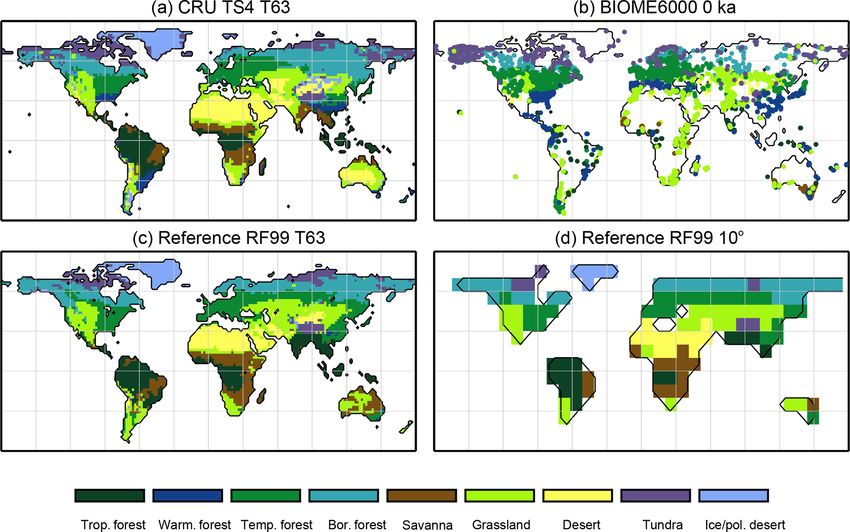
342                                                                 A. Dallmeyer et al.: Harmonising plant functional type distributions

Figure 2. Reference biome distributions for the pre-industrial time slice, i.e. (a) the biome distribution inferred by BIOME1 that has been
forced by the CRU TS4 dataset (1901–1930), interpolated to a Gaussian T63 grid; (b) the pollen-based pre-industrial biome reconstructions
provided by the Biome6000 database (Harrison, 2017); (c, d) the modern potential natural vegetation map derived by Ramankutty and Fo-
ley (1999, RF99) remapped on a T63 gaussian grid (c) and a 10◦ grid (d). The biomes are tropical forest (trop.forest), warm–temperate forest
(warm.forest), temperate forest (temp.forest), boreal forest (bor.forest), savanna and dry woodland (savanna), grassland and dry shrubland
(grassland), warm desert (desert), tundra (tundra) and polar desert and ice (ice/pol.desert).

2.4.3    Best neighbour score                                               hood. It is equal to 1 if the grid box locating the site indi-
                                                                            cates the same biome as reconstructed and it is equal to 0 if
Neither the FSS nor the fuzzy kappa statistic is in its original            all grid cells in the neighbourhood disagree with the record.
format applicable for the comparison of site data vs. gridded               The BNS is the mean of all individual neighbourhood scores.
data. For quantifying the similarity of simulated biome dis-                For instance, a BNS of approximately 0.82 or 0.46 means
tributions and pollen-based biome reconstructions, we there-                that the best neighbour grid cell is among the grid cell “cir-
fore implement a new metric following both methods called                   cle” next to the site-locating grid cell in T63 or T31, respec-
the best neighbour score (BNS), accounting for agreement                    tively. Accordingly, a BNS of 0.04 indicates a distance be-
in the neighbourhood of the record site and therewith being                 tween the best neighbour and the site-locating grid cell of
more tolerant of the position of the site. Within this metric,              7.5◦ on a Gaussian grid. In contrast to the fuzzy kappa statis-
not only the grid box locating the record sites is used for                 tic, the BNS neither takes agreement by chance into account
comparison with the records but also the surrounding grid                   nor considers potential spatiotemporal autocorrelation.
boxes (three grid boxes in each direction for T31, six for T63,                At this point it should be noted that we have selected
one for a 10◦ grid). Similar to the fuzzy kappa statistic, the              the metrics in accordance with the research question of this
similarity in the neighbouring grid cells is expressed by a                 study. For other purposes, such as estimating changes in
distance decay function. We here choose a Gaussian func-                    biome distribution between present and future climate states,
tion (Eq. 4), giving grid cells directly at the site proportional           other metrics may be more appropriate, such as the Delta-V
larger influence than grid boxes far away.                                  method, which also weights changes in vegetation attributes

        −1 distance
                      2                     q                              (Sykes et al., 1999). The metrics used in our study do not dif-
        2 ·
w=e            3
                           with distance =       d long2 + d lat2   (4)     ferentiate how far the biomes deviate in their properties; e.g.
                                                                            differences between tropical forest and tundra are equated as
The best neighbour is defined as the nearest grid box within                being qualitatively the same as differences between temper-
the neighbourhood agreeing with the reconstructed biome                     ate and boreal forest.
type. The agreement for each record is then given by the dis-
tance weight (w) of the best neighbour in each neighbour-

Clim. Past, 15, 335–366, 2019                                                                          www.clim-past.net/15/335/2019/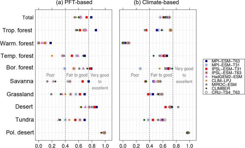
A. Dallmeyer et al.: Harmonising plant functional type distributions 343
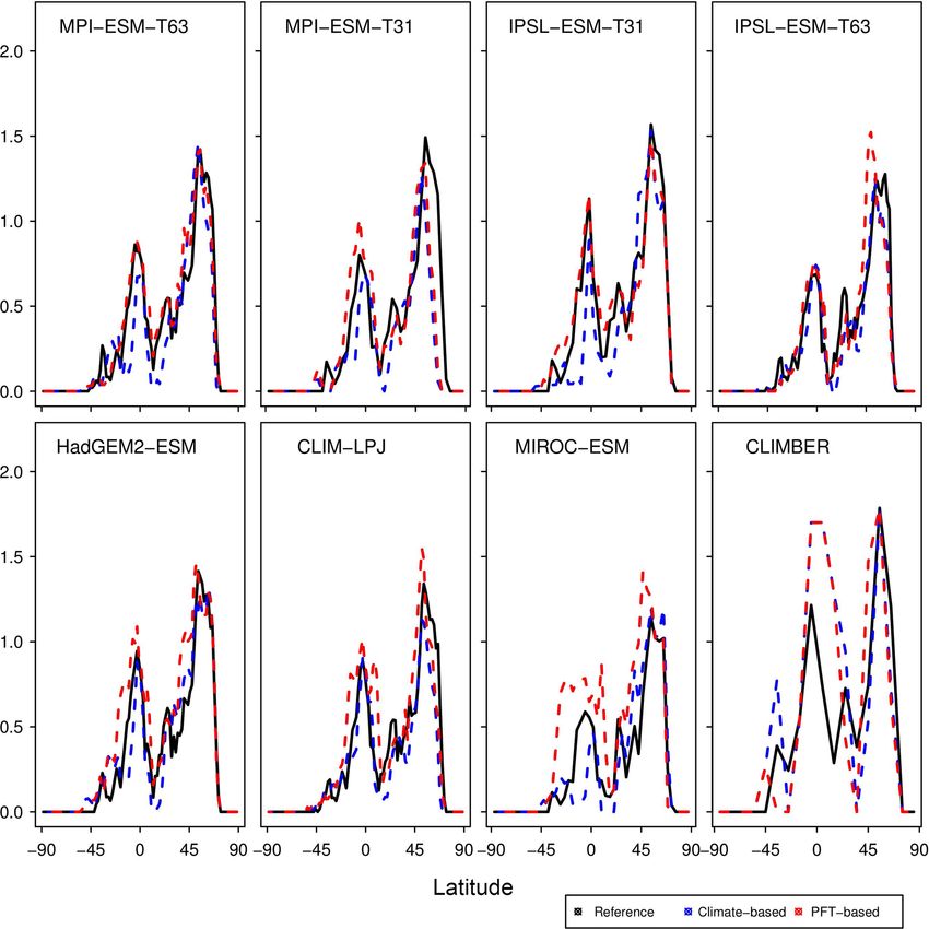
Figure 3. Simulated pre-industrial mega-biome distributions according to the new biomisation method (PFT-based method). The PFT frac-
tions simulated by the individual models have been converted into mega-biomes through climate limitation rules and assumptions on the
maximum coverage of certain PFTs needed in the grid cells.
3 Results etation models. The biomisation based on the PFT coverage
generally assigns more grid cells to forest or woody biomes
3.1 Comparison of the PFT-based and climate-based (e.g. savanna instead of grassland or desert) than the classi-
biome distributions for the pre-industrial time slice cal method. This is most noticeable in South America, where
the area covered by tropical forests is strongly increased in
For the pre-industrial time slice, the PFT coverage of eight the PFT-based biome distribution (Table D1), being more
different Earth system model simulations has been converted in line with observations. Likewise, the savanna and/or for-
into mega-biome distributions (Fig. 3). Additionally, the un- est biomes are more spread out on the African continent for
derlying pre-industrial climate states are used as forcing for nearly all biomisations with the exception of the CLIMate-
the BIOME1 model (i.e. the classical way of biomisation) to BiosphERe 2 (CLIMBER-2) model and IPSL-ESM-T63.
calculate the mega-biome distributions in equilibrium with The Asian forest regions are slightly larger in most PFT-
the simulated climate states (Fig. 4). Overall, the PFT-based based biome distributions compared to the climate-based
biome maps look similar to the climate-based ones. All ma- ones. This impression is reinforced by the fact that for CLIM-
jor biome belts can be reproduced using the new method, LPJ and IPSL-ESM-T63 the PFT method suggests a pro-
independent of the resolution or the complexity of the veg-
www.clim-past.net/15/335/2019/ Clim. Past, 15, 335–366, 2019
344                                                          A. Dallmeyer et al.: Harmonising plant functional type distributions

Figure 4. Simulated pre-industrial biome distributions according to the classical biomisation approach, i.e. biomising the climate states
simulated by the individual models. The climate field were used to force the biome model BIOME1 (Prentice et al., 1992). Afterwards, the
original BIOME1 biomes were aggregated into the nine mega-biomes used in this study.

nounced boreal forest belt in northern Asia, not only reducing         biomisation methods, biases related to the imperfect vege-
the size of the grassland but also that of the temperate forest        tation models or biases in the simulated climate. While the
area.                                                                  effect of shortcomings in the vegetation models cannot be
   For North America, the PFT-based approach yields less               disentangled, the caveats of the PFT-based method and the
forest for MPI-ESM-T63 and IPSL-ESM-T31 than shown by                  effect of climate biases on the PFT-to-biome conversion are
the climate-based biomisation. As a consequence, the North             further discussed in Sect. 4.
American prairie fits better to observations for the PFT-based
biome distributions. In Alaska and north-western Canada,               3.2   Quantitative comparison of the PFT-based biome
parts of the tundra regions suggested by BIOME1 tend to                      distributions with reference biome maps
be replaced by boreal forest when using the new approach,
which is generally more consistent with the observed vegeta-           To quantify the skill of the new method to represent the
tion.                                                                  global biome distribution, we compare the resulting biome
   The differences between the PFT-based and climate-based             maps with the modern potential natural vegetation cover esti-
biome distributions can be caused by deficiencies in the               mated by Ramankutty and Foley (1999, RF99 in the follow-
                                                                       ing) and the pre-industrial biome reconstructions provided

Clim. Past, 15, 335–366, 2019                                                                       www.clim-past.net/15/335/2019/
A. Dallmeyer et al.: Harmonising plant functional type distributions 345 Figure 5. Metrics quantifying the total agreement of the simulated pre-industrial biome maps based on the PFT cover fractions (PFT method) or based on the climate state (classical approach using BIOME1) with the reference datasets, i.e. modern potential natural vegetation (RF) and pre-industrial pollen-based biome reconstructions (rec.). Shown are the kappa values (a), the relative fractional skill score (FSS, b) and the best neighbour score (BNS, c) for all models and also for the biomisation based on the CRU TS4 observational climate data in original resolution (CRU TS4) and interpolated to a T63 grid (CRU TS4_T63). by the Biome6000 project (Harrison, 2017). As target for the ESM-T31, HadGEM2-ESM and CLIMBER biomisations, skill, the level of agreement between the BIOME1 derived the PFT-based method even produces biome distributions biome distribution of the observed climate (CRU TS4, 1901– that fit better to the biome reconstructions than the climate- 1930; cf. Fig. 2) and the reference datasets is taken, i.e. κ of based biome maps. 0.68 and FSS of 0.13 (Fig. 5) with respect to RF99 and a κ of Despite the overall agreement between the PFT-based 0.46 and BNS of 0.73 with respect to the biome reconstruc- biome distributions and the references, a closer look at the tions. representation of individual mega-biomes in the converted The PFT-based biome distributions agree well with the ref- maps indicates large differences among the models as well erences, independent of the model. The kappa statistic shows as among the individual mega-biomes (Fig. 6). While trop- an overall agreement to RF99 between 0.54 (for MIROC- ical forests and deserts compare best with RF99, the biome ESM) and 0.79 (for MPI-ESM-T63) revealing a good to very “warm–temperate forest” is not reproduced, independent of good agreement (Fig. 5). Likewise, all models reach in total the underlying model simulation. the level of good skill in the FSS metric (0.01–0.27). This The skill for simulating the other biomes is very different agreement is in line with or even better than the match be- for the diverse models. κ spreads from poor for one model tween RF99 and the climate-based biomisation and that be- to very good for other models. Correcting the PFT distribu- tween RF99 and the CRU TS4 biomisation that is taken as tion in land-use areas by redistributing the area fraction to the the target skill (Fig. 5). However, the spread between the in- other tiles has no impact on the performance of the method. dividual models is larger for the PFT-based method than for The biome maps based on simulations applying land use do the classical approach. not compare worse with RF99 than the maps of other sim- As expected, the kappa statistic indicates that the PFT- ulations. Likewise, the complexity of the vegetation model based biome maps compare worse with the reconstructions and the number of distinguished PFTs have no significant ef- than with RF99, underestimating the similarity to the point fect on the representation of the biome distribution, indicat- reconstructions. κ ranges from 0.2 (poor) to 0.49 (fair), ing that the climate limits used in the biomisation procedure which is in line with the target skill and the metrics for the are appropriate for the assignment of the PFTs to the dis- climate-based biome maps. The BNS, additionally consid- tinct PFT groups. The differentiation of the PFT types (e.g. ering accordance in the neighbouring grid cells of the record the different forest types) in vegetation models is often based sites, reveals a good to very good agreement of the PFT-based on similar climate limits, regardless of whether the model biome distributions and the records (between 0.40 and 0.74), is a complex dynamic vegetation model or a simple biome not much lower than the target skill and in accordance with model. With the exception of the PFT-based biomisation for the climate-based biomisations. For the MPI-ESM, IPSL- CLIMBER, in which the coarse grid is clearly disadvanta- www.clim-past.net/15/335/2019/ Clim. Past, 15, 335–366, 2019
346                                                          A. Dallmeyer et al.: Harmonising plant functional type distributions

Figure 6. Kappa metric quantifying the agreement of the simulated pre-industrial individual mega-biomes with the reference dataset (i.e.
modern potential natural vegetation) for the PFT-based method (a) and the classical method using BIOME1 forced with the simulated
background climate states (b).

geous for capturing the reconstructed desert belts and the            3.3   PFT-based biome distributions for the mid-Holocene
rather regionally confined biomes (savanna, warm–temperate                  and Last Glacial Maximum time slice
forest), the spatial resolution of the models is not the primary
                                                                      The sensitivity of the PFT-based method to changes in the
factor for the spread in the metrics. The PFT-based method
                                                                      vegetation cover is assessed by evaluating palaeo-biome dis-
performs equally well for simulations using T63 as for sim-
                                                                      tributions. For the mid-Holocene time slice, four differ-
ulations using T31 (in total); only the regionally distributed
                                                                      ent simulations have been analysed. The main vegetation
warm–temperate forest is better represented in finer resolu-
                                                                      changes described by biome reconstructions are the northern
tions.
                                                                      shift of the Northern Hemisphere forest belts, in particular
   In general, the skill in representing the individual mega-
                                                                      a northward displacement of the taiga–tundra boundary, and
biomes is similar for the PFT- and climate-based meth-
                                                                      the decrease of the desert areas compared to pre-industrial
ods. Both approaches have the same strengths and weak-
                                                                      time slice. According to the BIOME6000 records, grassy
nesses, but the spread between the models is larger for
                                                                      vegetation reached at least up to 26◦ N at 6 ka, far into the
the PFT-based biomisations. In comparison to the climate-
                                                                      modern central Sahara (Fig. 7). For none of the models is this
based method, the tropical, the warm–temperate and the bo-
                                                                      biome shift reproduced, neither in the PFT-based (Fig. 7) nor
real forest biomes tend to be slightly better represented by
                                                                      in the climate-based biome distributions (not shown). The
the PFT-based method. In contrast, the temperate forest, sa-
                                                                      mean Sahara desert border shifts northward by one to two
vanna and grassland distribution – averaged over all mod-
                                                                      grid cells in the biomisations (i.e. approximately 1.875 to
els – fit better to RF99 when using the climate-based ap-
                                                                      3.75◦ , Table 4). This shift collocates with substantial reduc-
proach, although for individual simulations, κ derived for the
                                                                      tions in the desert fractions simulated by the individual ESMs
PFT biomisation exceeds the climate-based one. The savanna
                                                                      (Fig. 8). Only in MPI-ESM-T63 is vegetation increased in the
and grassland biomes are particularly misrepresented in the
                                                                      entire western and central Sahara, but this increase is lower
biome maps that are based on the PFT distributions simulated
                                                                      than 20 %, not leading to a change in the biome assignment
by MIROC-ESM, CLIMBER, CLIM-LPJ and HadGEM2-
                                                                      from desert to grassland. As the climate-based biomisations
ESM. The temperate forest is poorly reproduced only in the
                                                                      performed with BIOME1 reveal a reduction of the Sahara
PFT-based biomisation of CLIM-LPJ. Overall, the metrics
                                                                      desert area in the same magnitude as the PFT-based ones, we
indicate that the PFT-based method works as well as the clas-
                                                                      conclude that the new biomisation method shows a reason-
sical approach of biomising climate states via the BIOME1
                                                                      able sensitivity to the simulated changes in the desert frac-
model. Likewise, the method is able to keep up with the
                                                                      tions.
method by Prentice et al. (2011), further discussed in Ap-
pendix E.

Clim. Past, 15, 335–366, 2019                                                                      www.clim-past.net/15/335/2019/
A. Dallmeyer et al.: Harmonising plant functional type distributions 347 Figure 7. Simulated mid-Holocene biome distribution in the different models, based on the PFT method (a), pollen-based biome reconstruc- tions of the mid-Holocene biome distribution (BIOME6000 database, b) and the best neighbour score (BNS) for all individual sites showing the agreement of the reconstructed biomes and the biome distribution in the neighbourhood of the sites, ranging from 0 (no grid cell in the surrounding area shows the same biome as reconstructed) to 1 (the grid cell locating the site and the record at the site indicate the same biome) (c). For all models with the exception of MIROC-ESM, the reconstructions (Table 5). However, the magnitude of the PFT-based biomisation reproduces an increased forest biome change differs between the models, ranging from 0 % within fraction in Eurasia north of 60◦ N during the mid-Holocene MIROC-ESM to 12 % within CLIM-LPJ. For nearly all mod- compared to pre-industrial time slice, in line with the biome els (except for MIROC-ESM), the expansion of the forested www.clim-past.net/15/335/2019/ Clim. Past, 15, 335–366, 2019
348                                                        A. Dallmeyer et al.: Harmonising plant functional type distributions

Figure 8. Differences in the desert fractional coverage simulated by the individual models between the mid-Holocene (6 ka) and pre-
industrial time slices (0 ka).

area in the high northern latitudes seen in the PFT biomi-          biomisations mostly reproduce this reduction and the shift in
sation is of similar magnitude to that in the climate-based         Northern Hemisphere forest biomes (Fig. 10), though the ex-
biomisation, confirming that the method covers past vegeta-         tent of the shift is underestimated. Forest reaches up to 50◦ N
tion changes with reasonable sensitivity.                           (for CLIMBER) to 65◦ N (for MPI-ESM-T63). The boreal
   Overall, the biome distributions for the mid-Holocene            forest position in the MIROC-ESM biomisation is not much
compare equally well to the reconstruction as they do for           changed compared to PI, but the boreal forest nearly replaces
the pre-industrial time slice (Fig. 9). Although κ is simi-         the temperate forest biome.
larly low, ranging from 0.17 for the CLIM-LPJ biomisation              The overall agreement of the PFT-based biome distribu-
to 0.38 for the MPI-ESM-T63 biomisation (poor agreement),           tions with the biome reconstructions is rather fair but in line
the spread in the models and the differences in κ between           with the results for the climate-based biome distributions. κ
the PFT-based biomisations and the climate-based biomisa-           ranges from 0.07 for MPI-ESM-T31 to 0.23 for CLIMBER,
tions is nearly identical to the results for the pre-industrial     only indicating a poor similarity of the biome maps and
biome distributions. In line with the results for PI, the BNS       records (Fig. 11). The BNS ranges from 0.24 (for MIROC-
indicates a good to very good agreement to the biome re-            ESM) to 0.57 (for MPI-ESM-T63) revealing a fair to good
constructions (ranging from 0.44 for MIROC-ESM to 0.72              agreement. The values for both metrics are in the same mag-
for MPI-ESM-T63). The skill to capture the reconstructed            nitude as for the climate-based biomisations. Similar to the PI
individual mega-biomes strongly depends on the number of            time slice, neither the complexity nor the spatial resolution is
available pollen records; thus, temperate and boreal forests        the main reason for the differences between the PFT biomi-
are represented best (Fig. 7), while the simulated savanna re-      sations. The spread in the skill of representing the individual
gions are not supported by the biome reconstructions.               biomes is large, and no systematic bias for one model can be
   For the Last Glacial Maximum time slice, five different          found. With the exception of the biomisation for CLIMBER,
simulations have been analysed. According to BIOME6000,             the savanna biome is misrepresented in all biomisations, in-
the main reconstructed vegetation differences at LGM com-           dependent of whether the PFT-based or the climate-based
pared to PI are a strong equatorward retreat of the forest          method was used. Within the model ensemble, tropical and
biomes and an expansion of tundra and steppe regions. The           temperate forest can be reproduced best.
northernmost record indicating boreal forest during LGM is
located at approximately 51◦ N in Asia (Fig. 10). The PFT

Clim. Past, 15, 335–366, 2019                                                                   www.clim-past.net/15/335/2019/
A. Dallmeyer et al.: Harmonising plant functional type distributions                                                             349

Figure 9. Metrics quantifying the agreement of the simulated mid-Holocene biome maps based on the PFT method or based on the climate
states (i.e. according to the BIOME1 model) with the pollen-based biome reconstructions (BIOME6000 database) for the mid-Holocene time
slice, i.e. the (total) kappa value (left panel) and the BNS values for the individual mega-biomes.

Figure 10. Pollen-based biome reconstructions (BIOME6000 database) for the Last Glacial Maximum time slice and the simulated biome
distributions according to the new biomisation method (i.e. the PFT-based method).

www.clim-past.net/15/335/2019/                                                                      Clim. Past, 15, 335–366, 2019
350                                                              A. Dallmeyer et al.: Harmonising plant functional type distributions

Table 4. Position of the desert margin (◦ latitude) in north Africa at PI and 6 ka and the differences in position of the desert margin between
6 ka and PI (◦ latitude), for the PFT-based biomisations and the climate-based biomisations. The desert margin is here defined as latitude at
which the zonal mean desert biome fraction averaged over the region 15◦ W to 30◦ E exceeds 50 %.

                                                               PFT-based                   Climate-based
                                                         PI      6 ka   6 ka–PI        PI      6 ka     6 ka–PI
                                 MPI-ESM-T63          17.72     21.45        3.73   15.85     19.59        3.74
                                 CLIM-LPJ             15.85     17.72        1.87   17.72     21.45        3.73
                                 HadGEM2-ESM          13.99     15.85        1.86   13.99     15.85        1.86
                                 MIROC-ESM             16.7     20.41        3.71    16.7     20.41        3.71

Table 5. Mean forest biome fraction in northern Eurasia (60–80◦ N, 0–150◦ E) in the PFT-based biomisations and the climate-based biomi-
sations for the mid-Holocene (6 ka) and pre-industrial (PI) time slice, and the difference between both (6 ka–PI).

                                                                PFT-based               Climate-based
                                                          PI     6 ka   6 ka–PI       PI     6 ka     6 ka–PI
                                   MPI-ESM-T63          0.73     0.75        0.02   0.73    0.76        0.03
                                   CLIM-LPJ             0.64     0.76        0.12   0.67    0.77         0.1
                                   HadGEM2-ESM          0.83     0.89        0.06   0.89    0.93        0.04
                                   MIROC-ESM            0.72     0.72         0.0   0.92    0.96        0.04

4     Discussion                                                            adopt the bioclimatic limits from BIOME4 (limit for tem-
                                                                            perate evergreen broadleaved trees) for defining this mega-
4.1    Caveats in the method                                                biome. Nevertheless, the calculated warm–temperate forest
                                                                            distribution strongly disagrees with the reference datasets.
Even if the biomisation is restricted to mega-biome level, no               The reconstructed biome “warm–temperate forest” shares
clear definitions exist to distinguish biomes in terms of plant             some subtropical PFTs with the tropical evergreen forest (Ni
functional type compositions. While the bioclimatic limits                  et al., 2010). These biomes are quite different in key species,
used in the biome models are based on empirical analysis, no                but not on genus or family level, on which the pollen iden-
equivalent classification regulates the biomisation of PFTs.                tification in the reconstructions is performed. Thus, these
We particularly face this problem in finding a meaningful                   biomes tend to overlap in some regions and are sometimes
threshold of maximum tree cover needed for defining forests.                mixed up in reconstructions (Chen et al., 2010). In addition,
When is an accumulation of trees identified as forest? As                   this mega-biome includes the warm–temperate rainforest and
models tend to underestimate the forest coverage and forest                 the wet sclerophyll forest and woodland in the BIOME6000
extent in the high northern latitudes (cf. Loranty et al., 2013),           reconstructions (cf. Harrison, 2017), which may not be able
we choose the assumption of tree cover being just dominant                  to be identified with our biomisation method. Regarding the
in forested grid cells, although this limit is very low. We test            modern reference of RF99, we decided to assign the biome
other limits (e.g. absolute dominance, i.e. fractional coverage             “temperate needleleaf evergreen forest and woodland” of the
exceeding 50 %), but these work worse for most simulations                  RF99 dataset to the mega-biome “temperate forest”, although
used in this study as well as for other simulations.                        this biome is also located, e.g. in the southern US, which
   The mega-biome “warm–temperate forest” (e.g. subtrop-                    should be assigned to the warm–temperate forest. There-
ical forest) includes PFTs that can be assigned to several                  fore, the evaluation of this method with respect to warm–
biomes and is rather defined by a coexistence of certain                    temperate forest might be ambiguous. Furthermore, warm–
PFTs. For instance, in the BIOME4 model, it is not only de-                 temperate forests are small and rather patchily distributed
fined by the dominance of temperate evergreen broadleaved                   and are thus rarely dominant in the coarse grid cells to which
trees but can also be defined by a dominance of cool conifers               the RF99 reference had to be interpolated to. The coarser
(with a sub-PFT of temperate evergreen broadleaved trees).                  the grid is, the more warm–temperate forest regions get lost
The cool conifers – in turn – are also part of temperate forest             during the interpolation. Therefore, the warm–temperate for-
biomes. Given the limited number of PFTs in the DGVMs,                      est biome is generally better represented for models using a
the confinement of biomes via PFT mixtures is not possi-                    higher spatial resolution (i.e. MPI-ESM-T63, CLIM-LPJ and
ble. As biome models such as BIOME4 generally manage to                     IPSL-ESM-T63).
simulate warm–temperate forests at the correct locations, we

Clim. Past, 15, 335–366, 2019                                                                              www.clim-past.net/15/335/2019/
You can also read