AUTOMATIC QUESTION PARAPHRASING IN SWEDISH WITH DEEP GENERATIVE MODELS - DIVA
←
→
Page content transcription
If your browser does not render page correctly, please read the page content below

DEGREE PROJECT IN THE FIELD OF TECHNOLOGY
INFORMATION AND COMMUNICATION TECHNOLOGY
AND THE MAIN FIELD OF STUDY
COMPUTER SCIENCE AND ENGINEERING,
SECOND CYCLE, 30 CREDITS
STOCKHOLM, SWEDEN 2021

Automatic Question Paraphrasing
in Swedish with Deep Generative
Models

NIKLAS LINDQVIST

KTH ROYAL INSTITUTE OF TECHNOLOGY
SCHOOL OF ELECTRICAL ENGINEERING AND COMPUTER SCIENCE
Automatic Question
Paraphrasing in Swedish with
Deep Generative Models

NIKLAS LINDQVIST

Master’s Programme, Machine Learning, 120 credits
Date: April 1, 2021
Supervisor: Dmytro Kalpakchi
Examiner: Viggo Kann
School of Electrical Engineering and Computer Science
Swedish title: Automatisk frågeparafrasering på svenska med
djupa generativa modeller
Abstract | i

Abstract
Paraphrase generation refers to the task of automatically generating a para-
phrase given an input sentence or text. Paraphrase generation is a fundamental
yet challenging natural language processing (NLP) task and is utilized in
a variety of applications such as question answering, information retrieval,
conversational systems etc.
    In this study, we address the problem of paraphrase generation of questions
in Swedish by evaluating two different deep generative models that have shown
promising results on paraphrase generation of questions in English. The first
model is a Conditional Variational Autoencoder (C-VAE) and the other model
is an extension of the first one where a discriminator network is introduced
into the model to form a Generative Adversarial Network (GAN) architecture.
In addition to these models, a method not based on machine-learning was
implemented to act as a baseline. The models were evaluated using both
quantitative and qualitative measures including grammatical correctness and
equivalence to source question.
    The results show that the deep generative models outperformed the
baseline across all quantitative metrics. Furthermore, from the qualitative
evaluation it was shown that the deep generative models outperformed the
baseline at generating grammatically correct sentences, but there was no
noticeable difference in terms of equivalence to the source question between
the models.

Keywords
Paraphrase Generation, Variational Autoencoder, Generative Adversarial Net-
works, Natural Language Generation, Deep Learning, Word Embeddings
ii | Sammanfattning
Sammanfattning
Parafrasgenerering syftar på uppgiften att, utifrån en given mening eller text,
automatiskt generera en parafras, det vill säga en annan text med samma
betydelse. Parafrasgenerering är en grundläggande men ändå utmanande
uppgift inom naturlig språkbehandling och används i en rad olika applikationer
som informationssökning, konversionssystem, att besvara frågor givet en text
etc.
I den här studien undersöker vi problemet med parafrasgenerering av
frågor på svenska genom att utvärdera två olika djupa generativa modeller som
visat lovande resultat på parafrasgenerering av frågor på engelska. Den första
modellen är en villkorsbaserad variationsautokodare (C-VAE). Den andra
modellen är också en C-VAE men introducerar även en diskriminator vilket gör
modellen till ett generativt motståndarnätverk (GAN). Förutom modellerna
presenterade ovan, implementerades även en icke maskininlärningsbaserad
metod som en baslinje. Modellerna utvärderades med både kvantitativa och
kvalitativa mått inklusive grammatisk korrekthet och likvärdighet mellan
parafras och originalfråga.
Resultaten visar att de djupa generativa modellerna presterar bättre än
baslinjemodellen på alla kvantitativa mätvärden. Vidare, visade the kvalitativa
utvärderingen att de djupa generativa modellerna kunde generera grammatiskt
korrekta frågor i större utsträckning än baslinjemodellen. Det var däremot
ingen större skillnad i semantisk ekvivalens mellan parafras och originalfråga
för de olika modellerna.
Nyckelord
Parafrasgenerering, Variational Autoencoder, generativa adversariala nätverk,
naturlig språkgenerering, djupinlärning, ordinbäddningAcknowledgments | iii Acknowledgments I would like to direct a huge "thank you" to my supervisor, Dmytro Kalpakchi, for his guidance throughout this thesis. I am so grateful for his genuine interest in this thesis which have resulted in the numerous hours of interesting and learning discussions which have turned this thesis into something that would not have been possible otherwise. I would also like to thank Johan Boye for helping me find such an interesting topic for my thesis. Last but not least, I would like to thank my parents for always being there for me and supporting me in everything I do. It would have not been possible without them. Thank you! Stockholm, April 2021 Niklas Lindqvist
iv | CONTENTS

Contents

1   Introduction                                                                                         1
    1.1 Problem Statement . . . . . . . . .      .   .   .   .   .   .   .   .   .   .   .   .   .   .   2
    1.2 Purpose . . . . . . . . . . . . . . .    .   .   .   .   .   .   .   .   .   .   .   .   .   .   3
    1.3 Objective . . . . . . . . . . . . . .    .   .   .   .   .   .   .   .   .   .   .   .   .   .   3
    1.4 Delimitations . . . . . . . . . . . .    .   .   .   .   .   .   .   .   .   .   .   .   .   .   3
    1.5 Societal and Ethical Considerations      .   .   .   .   .   .   .   .   .   .   .   .   .   .   3
    1.6 Sustainability . . . . . . . . . . . .   .   .   .   .   .   .   .   .   .   .   .   .   .   .   4
    1.7 Thesis Outline . . . . . . . . . . . .   .   .   .   .   .   .   .   .   .   .   .   .   .   .   4

2   Background                                                                                            5
    2.1 Artificial Neural Networks . . . . . . . .           .   .   .   .   .   .   .   .   .   .   .    5
        2.1.1 Multi-Layer Perceptron . . . . . .             .   .   .   .   .   .   .   .   .   .   .    6
        2.1.2 Highway Networks . . . . . . . .               .   .   .   .   .   .   .   .   .   .   .    9
        2.1.3 Recurrent Neural Networks . . . .              .   .   .   .   .   .   .   .   .   .   .    9
        2.1.4 Variational Autoencoder . . . . .              .   .   .   .   .   .   .   .   .   .   .   12
        2.1.5 Generative Adversarial Networks                .   .   .   .   .   .   .   .   .   .   .   15
    2.2 Word Embeddings . . . . . . . . . . . .              .   .   .   .   .   .   .   .   .   .   .   16
        2.2.1 fastText . . . . . . . . . . . . . .           .   .   .   .   .   .   .   .   .   .   .   17
    2.3 Google’s Neural Machine Translation . .              .   .   .   .   .   .   .   .   .   .   .   18
    2.4 Evaluation Metrics . . . . . . . . . . . .           .   .   .   .   .   .   .   .   .   .   .   19
        2.4.1 BLEU . . . . . . . . . . . . . . .             .   .   .   .   .   .   .   .   .   .   .   19
        2.4.2 METEOR . . . . . . . . . . . . .               .   .   .   .   .   .   .   .   .   .   .   20
        2.4.3 TER . . . . . . . . . . . . . . . .            .   .   .   .   .   .   .   .   .   .   .   21

3   Related Work                                                                                         23
    3.1 Traditional Paraphrase Generation . .        .   .   .   .   .   .   .   .   .   .   .   .   .   23
    3.2 Deep Learning Approaches . . . . . .         .   .   .   .   .   .   .   .   .   .   .   .   .   24
         3.2.1 Sequence-to-sequence Models           .   .   .   .   .   .   .   .   .   .   .   .   .   24
         3.2.2 Deep Generative Models . . .          .   .   .   .   .   .   .   .   .   .   .   .   .   26
Contents | v
3.2.3 Reinforcement Learning Models . . . . . . . . . . . . 31
4 Methods 32
4.1 Dataset . . . . . . . . . . . . . . . . . . . . . . . . . . . . . 32
4.2 Data Preparation . . . . . . . . . . . . . . . . . . . . . . . . 33
4.2.1 Data Filtering and Translation . . . . . . . . . . . . . 33
4.2.2 Data Partitioning . . . . . . . . . . . . . . . . . . . . 34
4.3 Models . . . . . . . . . . . . . . . . . . . . . . . . . . . . . 34
4.3.1 C-VAE Paraphraser . . . . . . . . . . . . . . . . . . . 35
4.3.2 GAN Paraphraser . . . . . . . . . . . . . . . . . . . . 37
4.4 Baseline . . . . . . . . . . . . . . . . . . . . . . . . . . . . . 37
4.4.1 Synonym Paraphraser . . . . . . . . . . . . . . . . . 38
4.4.2 Implementation Details . . . . . . . . . . . . . . . . . 38
4.5 Evaluation . . . . . . . . . . . . . . . . . . . . . . . . . . . . 40
5 Results 43
5.1 Quantitative Model Evaluation . . . . . . . . . . . . . . . . . 43
5.2 Qualitative Model Evaluation . . . . . . . . . . . . . . . . . . 46
5.3 Quality of Data . . . . . . . . . . . . . . . . . . . . . . . . . 49
5.4 Qualitative Samples . . . . . . . . . . . . . . . . . . . . . . . 50
6 Discussion 53
6.1 Deep Generative Models . . . . . . . . . . . . . . . . . . . . 53
6.1.1 Hyper-parameter tuning . . . . . . . . . . . . . . . . 53
6.1.2 Error analysis . . . . . . . . . . . . . . . . . . . . . . 54
6.2 Baseline . . . . . . . . . . . . . . . . . . . . . . . . . . . . . 54
6.2.1 Error analysis . . . . . . . . . . . . . . . . . . . . . . 54
6.3 Human Evaluation . . . . . . . . . . . . . . . . . . . . . . . 55
6.3.1 Error Analysis . . . . . . . . . . . . . . . . . . . . . 56
6.4 Future Work . . . . . . . . . . . . . . . . . . . . . . . . . . . 56
7 Conclusions 58
References 59
A Evaluation Instructions To The Human Judges 67
B Source Question With Grammatical Errors 69Introduction | 1
Chapter 1
Introduction
Paraphrases are defined as sentences or texts that in the same language
express the same semantic meaning but use different wordings. Paraphrase
generation refers to the task of automatically generating a paraphrase given
an input sentence or text. Paraphrase generation is a fundamental yet
challenging natural language processing (NLP) task and is utilized in a variety
of applications such as question answering [1], information retrieval [2],
conversational systems [3] etc.
Human language, both spoken and written, is typically full of paraphrases.
Thus, comprehending the semantic meaning of paraphrases is essential to
fully understand a language. One common way to test how well someone
understands the semantic meaning of a text is by doing reading comprehension
tests. Such tests are usually performed by reading a text and then answering a
set of multiple choice questions about that text.
As of today those reading comprehension tests are designed by humans,
which is a time-consuming task. One way to automate this task is by using
NLP techniques to extract question-answer pairs from the text. For example,
from the Swedish text:
En finansiell controller har som främsta uppgift att analysera dåtid
och nuläge i ekonomiska siffror. Att kunna läsa av resultat- och
måluppfyllnad och sedan rapportera till ledning samt till övriga i
organisationen är det viktigaste.
the question-answer pair
Q: Vad har en finansiell controller som främsta uppgift?
A: Att analysera dåtid och nuläge i ekonomiska siffror.
could be generated, which in English translates to2 | Introduction
A financial controller’s main task is to analyze the past and present
situation in financial figures. Being able to read results and goal
fulfillment and then report to management and to others in the
organization is the most important thing.
and the question-answer pair
Q: What is a financial controller’s main task?
A: To analyze the past and present situation in financial figures.
However, stating a question word by word from the text will test not reading
comprehension skills, but pattern matching skills instead. To overcome this
problem, a paraphrase to the question could be generated. For example, from
the question
"Vad har en finansiell controller som främsta uppgift?" (eng.
"What is a financial controller’s main task?" )
the question
"Vilken uppgift utför en finansiell controller framförallt?" (eng.
"What task does a financial controller perform especially?")
could be generated. A similar technique can be used to paraphrase the answer.
1.1 Problem Statement
This thesis addresses the problem of automatically generating paraphrases
of questions in Swedish. The problem is addressed by implementing and
evaluating a few already existing machine learning (ML) methods for automatic
paraphrase generation in English. These methods have already proved to
be successful in question paraphrasing as they can produce well-formed,
grammatically correct paraphrase [4, 5, 6] . However, it is difficult to say how
effective these methods are when applied to other languages, such as Swedish.
The research question that will be addressed in this thesis is:
How do state-of-the-art ML-based paraphrase generation methods
perform when applied to Swedish questions and how do they
compare to traditional non-ML-based methods?
The hypothesis is that the machine-learning-based methods will outperform
traditional paraphrase generation methods based on hand-written rules.Introduction | 3 1.2 Purpose One of the research projects at KTH addresses the problem of automatically generating reading comprehension questions for Swedish texts. Such a problem can be divided into several sub problems where one is to automatically paraphrase basic questions, generated from a text. Thus, the purpose of this thesis is to propose a method for automatic paraphrase generation for questions in Swedish. 1.3 Objective The objective of this thesis is to implement systems for automatic question paraphrasing in Swedish by using modern machine learning (ML) techniques and compare its performance against a traditional non-ML-based system. This will be done by selecting a few of the today’s state-of-the-art ML methods for automatic question paraphrasing to implement and evaluate their performances on questions stated in Swedish. 1.4 Delimitations One limitation of this thesis is that no sufficiently large question dataset exists in Swedish and it is out of scope for this project to collect and create one ourselves. Therefore the English Quora Question Pairs dataset will be translated into Swedish and used for training. Although machine translation have made great improvements over the last years it is still not perfect which may result in a dataset of lower quality than the original Quora Question Pairs dataset. Due to time constraint, it is also out of scope for this project to do a proper hyper-parameter tuning for the models that are being implemented. Instead the same parameter setting as in the original articles will be used. 1.5 Societal and Ethical Considerations The ethical discussion in data science today is mainly centered around privacy concerns [7]. Historically, NLP have mostly involved processing text that were usually published publicly, not linked to a specific author or had some temporal distance, thus creating distance between the author and the text [8]. Because of this, NLP have not really been a part of the discussion. However, over the last years more data are collected from social media and the applications of
4 | Introduction

NLP can now on a daily basis directly affect peoples lives [8]. As the Quora
Question Pairs dataset used in this thesis is made up of anonymous question-
pairs it is not violating the authors’ privacy or anonymity.
     The thesis itself will not have a direct societal impact, however the task of
paraphrase generation and natural language generation (NLG) in general can
have great societal impact if successfully implemented into applications such
as QA-systems, conversational systems or text summarization etc. Specifically
for this thesis, it potentially could contribute into a system which automatically
could generate reading comprehension tests, thus increase efficiency of
teachers and other people that today spend time creating those tests by hand.

1.6      Sustainability
Deep learning models have recently entered the field of NLP and have
outperformed state-of-the-art models across several fundamental NLP tasks
[9, 10, 11, 12]. There is also a strong relation between model complexity,
i.e. number of model parameters, and performance [13, 14, 15, 16] . Thus,
making the deep learning models energy-consuming to train which both have
a financial and environmental cost.
    The aim of this thesis is not to directly contribute to a more sustainable
environment and the models covered are computationally expensive to train
and are done so using graphical processing units (GPUs). However, this
computationally expensive training is only done once and when the models
are trained they are relatively cheap to run during inference.

1.7      Thesis Outline
In Chapter 2 the reader is presented with theory of the relevant deep learning
architectures and NLP models from which this thesis and the related work is
based upon. The last section of this chapter will also introduce the reader
with a few automatic evaluation metrics which are commonly used in the field
and will be used as a part of the evaluation for this thesis. Chapter 3 presents
related work including different paraphrase generation methods, with two of
them being evaluated in this thesis. Chapter 4 explains the methods used to
implement and evaluate the selected paraphrase generation models. Chapter 5
presents the results which are then analyzed and discussed further in Chapter 6
along with propositions of future work. Finally, in Chapter 7 the reader is
presented with the conclusions.
Background | 5
Chapter 2
Background
In this chapter, theory relevant to this thesis is presented. Section 2.1
introduces Artificial Neural Networks (ANNs) and their variations used in this
work. In Section 2.2, the reader will be introduced to the concept of word
embeddings and how it relates to ANNs. Section 2.3 presents the widely used
translation tool, Google’s Neural Machine Translation. Finally, in Section 2.4
the reader will be presented with some of the automatic metrics commonly
used in evaluation of paraphrase generation tasks. Before continuing, we
should present some notation used throughout this thesis to make it easier for
the reader to follow along. Lowercase letters in bold (e.g. a) denote vectors.
Capital letters in bold (e.g. A) denote matrices. Subscripts are used to denote
specific elements in a matrix or vector (e.g ai for the i:th element in a).
2.1 Artificial Neural Networks
Artificial neural networks (ANN) are a set of machine learning models
inspired by biological neural networks [17]. The main components of an ANN
are the computational units referred to as (artificial) neurons. The neurons
are interconnected with each other in structured ways to create the network
architecture. A neuron itself is essentially a function which takes some input
vector x = x1 , . . . , xN and produces an output o by performing a linear
operation followed by a non-linear one. Mathematically, a neuron j can be
described as:
N
X
f (x; wj , bj ) = a wji xi + bj (2.1)
i=16 | Background
where the weights wj and the bias term bj are the learnable parameters of an
ANN [18]. However, in the literature it is common to omit the bias term and
instead have an additional input dimension x0 set to one and the magnitude of
the bias stored in the weight w0 . The activation function is represented by a
and is needed to introduce non-linearity into the network. A few of the more
commonly used activation functions are presented in Equations 2.2-2.5.
The sigmoid function (see Equation 2.2) is an activation function which
maps the input to a value in the range (0, 1). Tanh (see Equation 2.3) has
similar shape to the sigmoid function but maps the inputs to values in the range
(-1, 1) instead. A rectified linear unit (ReLU) is a unit employing the rectifier
function (see Equation 2.4) which essentially outputs the maximum of 0 and
the input value. The softmax function (see Equation 2.5) is a generalization of
the sigmoid function and is often used as the last activation function in multi-
class classification networks to get a probability distribution over the output
classes.
1
Sigmoid: f (x) =σ(x) = (2.2)
1 + e−x
ex − e−x
Tanh: f (x) =tanh(x) = x (2.3)
( e + e−x
0 for x ≤ 0
ReLU: f (x) = = max(0, x) (2.4)
x for x > 0
exi
Softmax: fi (x) = PJ for i = 1, . . . , J (2.5)
xj
j=1 e
2.1.1 Multi-Layer Perceptron
The multi-layer perceptron (MLP) , also known as the feed-forward neural
network, is an ANN where the neurons are arranged into layers with connect-
ions only between adjacent layers [18]. In a fully-connected MLP each neuron
within a layer has directed connections to all neurons in the next layer, meaning
that the input to a neuron is all the outputs from the previous layer. This
results in a network architecture similar to a directed acyclic graph, as shown
in Figure 2.1. This network architecture allows the information to flow only in
one direction, from input to output, as opposed to Recurrent Neural Networks
which will be discussed in section 2.1.3.Background | 7
Figure 2.1 – An example of a feedforward neural network with one hidden
layer. The input layer is of size n, the hidden layer of size m and the output
layer of size 2.
Parameter Optimization
In an MLP, input data are fed to the network and propagated through the layers,
which produce an output in the last layer. For a classification problem this
output is usually a probability distribution over the classes. Training an MLP
essentially boils down to finding a set of network parameters θ such that the
error defined by some loss function is minimized. One of the most common
losses for training MLP-based classifiers is the cross-entropy loss defined in
Equation 2.6 where yi is a one-hot encoded target, which essentially is a vector
with a size equal to the number of classes with all values set to zero except for
the index corresponding to the correct class which is set to one. Furthermore,
pi is the output of the last layer which represents the network’s probability of
the input belonging to class i, and N is the number of classes.
N
1 X
cross entropy = − yi log pi (2.6)
N i=1
To make use of the loss defined by the loss function in order to update the
network parameters a method named back-propagation (or simply backprop)
can be used. Backprop was presented by Rumelhart et al. [19] in 1986 and uses
the chain rule to calculate partial derivatives of the loss function with respect8 | Background
to the networks’ parameters. As the name suggests these calculations are done
backwards through the network, from the last layer to the first. Once done,
the gradients can be used to update the network’s parameters using gradient
descent:
∂J(θt−1 )
θt = θt−1 − η (2.7)
∂θ
where θt is the networks’ parameters at iteration t, η the learning rate and
J(θ) a loss function. As the datasets grow larger it becomes time consuming
to calculate the loss and gradients which means training becomes very slow,
instead it is more common to use Stochastic Gradient Descent (SGD) which
each training iteration uses only a subset (also known as minibatch) of the
dataset.
Other optimization algorithms have been proposed to improve learning
further, one of them being Adam [20]. The name Adam is derived from
"adaptive moment estimation" and is an adaptive learning rate optimization
algorithm and was designed to combine the advantages of both other popular
methods, namely AdaGrad [21] and RMSProp [22]. Adam works by keeping
an exponentially decaying average of both past gradients and squared gradients
allowing it to adjust the learning rate for each parameter. Formally, it can be
described as:
gt =∇θ J(θt−1 ) (2.8)
mt =β1 · mt−1 + (1 − β1 ) · gt (2.9)
vt =β2 · vt−1 + (1 − β2 ) · gt2 (2.10)
mt
m̂t = (2.11)
1 − β1t
vt
v̂t = (2.12)
1 − β2t
m̂t
θt =θt−1 − η √ (2.13)
v̂t +
where mt is the biased first moment estimate and vt is the biased second
moment estimate. m̂t is the bias-corrected first moment estimate and likewise
v̂t the biased-corrected second moment estimate. β1 and β2 are hyper-
parameters of the Adam algorithm and are most commonly set to 0.999 and
0.9, respectively. Finally, is a small value, typically 1e-8 included to avoid
division by zero.Background | 9
2.1.2 Highway Networks
Highway networks were introduced in 2015 by Srivastava et al. [23] as a
method to overcome the problem of training very deep feed-forward neural
networks (FFNN). The architecture of the highway networks is inspired by the
Long Short-Term Memory which will be discussed later in Section 2.1.3.
In a plain L-layer FFNN, the l:th (l ∈ {1, 2, . . . , L}) layer applies a non-
linear activation function H to the product of the input vector x multiplied with
a weight matrix WH to produce an output vector y. The serialization of these
operations can together be referred to as a transformation, and mathematically
we can express such a transformation in layer l as:
yl = H(xl−1 , WHl ). (2.14)
The architecture of highway networks extend each layer in the FFNN by two
additional non-linear transformations T and C, parameterized by WT and WC ,
and after omitting the layer index for clarity, the results is:
y = H(x, WH ) · T (x, WT ) + x · C(x, WC ) (2.15)
where C is a carry gate as it decides how much of the original input is being
kept and sent to the output. In a similar way, T is the transform gate and
decides how much of the transformed input that is being sent to the output.
For simplicity, Srivastava et al. [23] suggest to use C = 1 − T thus resulting
in:
y = H(x, WH ) · T (x, WT ) + x · (1 − T (x, WT )). (2.16)
2.1.3 Recurrent Neural Networks
Feed-forward neural networks (FFNN) make the assumption that input data
points are independent of each other. This makes FFNNs inadequate for
processing sequential data such as sentences, i.e. a sequence of words, or
time series. Another lacking yet desirable property of the FFNNs is the
possibility to process sequences of different lengths as for example sentences
often differ in length. To resolve these limitations of FFNNs Recurrent Neural
Networks (RNNs) [19] were introduced. Cyclical connections between nodes
make it possible to introduce the notion of time which allows RNNs to share
parameters across several time steps. Figure 2.2 shows an RNN with one
hidden layer which is the simplest variation. As one can observe, the hidden10 | Background
(a) RNN as a circuit diagram. (b) RNN as an unfolded computational graph.
Figure 2.2 – An example of a recurrent neural network with an output at every
time step. Input x is fed into the network together with the hidden state of
previous step in order to produce an output y together with a new hidden state.
state ht is not only dependent on the input xt but also on ht−1 which is the
hidden state of the previous step allowing RNNs to memorize information
over several time steps.
The computations in the forward propagation differs from FFNNs as ht is
also dependent on previous time steps. Hence, the forward propagation can
formally be written as
at = Wxt + Uht−1 (2.17)
ht = tanh(at ) (2.18)
yt = sof tmax(Vht ) (2.19)
RNNs are trained using an extension of the back-propagation, namely back-
propagation through time (BPTT) which basically is the back-propagation
algorithm applied to the unrolled computational graph, shown in Figure 2.2b.
Although RNNs are able to learn short-term dependencies within seq-
uences, problems arise when relying on vanilla RNNs to learn long-term
dependencies. The problem is that gradients which are propagated through
many steps tend to either vanish (most commonly) or explode (more rarely)
[24]. Even if we assume that the networks are stable and that the gradients are
neither vanishing nor exploding the weights from the long-term dependencies
will be exponentially smaller than the short-term ones. This means in theory
that learning long-term dependencies will be really slow since these small
changes of weights will be hidden in recent short-term ones [24]. In practiceBackground | 11
though, experiments have shown that the probability of successfully training
a vanilla RNN with SGD is reaching zero for sequences of only length 10 or
20 when increasing the span of dependencies [25].
Several approaches have been taken to solve the problem of learning
long-term dependencies in RNNs by creating paths through time that have
derivatives that neither vanish nor explode. The most successful models which
accomplished this are called gated RNNs [24]. One of them being Long Short-
Term Memory (LSTM) [26].
Long Short-Term Memory
The Long Short-Term Memory (LSTM) model can more easily learn long-
term dependencies than simple RNNs and have thus shown to be successful
in multiple applications such as speech recognition, machine translation and
image captioning to name a few. The LSTM model solves the problem of
vanishing and exploding gradients by introducing cell states which have linear
self-loops between time steps. The linearity between these connections is
shown in Equation 2.23 where the new cell state is a linear combination of
the previous cell state and some new information defined in Equation 2.22.
The LSTM model makes use of different gates to control how the cell state is
updated through time steps. The gates that are present is a forget gate shown in
Equation 2.20 which controls how much information is kept from previous cell
state, an input gate (see Equation 2.21) which controls how much information
from the new cell state that should be added to the current cell state and finally
a output gate (see Equation 2.24) which controls how much of the current cell
state the output should be. Figure 2.3 shows an LSTM model over one time
step which gives an intuitive overview of the LSTM model. The forward pass
of an LSTM-cell is formally described in Equations 2.20-2.25.
ft =σ(Wf [xt , ht−1 ]) (2.20)
it =σ(Wi [xt , ht−1 ]) (2.21)
cet =tanh(Wc [xt , ht−1 ]) (2.22)
ct =ft ∗ ct−1 + it ∗ cet (2.23)
ot =σ(Wo [xt , ht−1 ]) (2.24)
ht =ot · tanh(ct ) (2.25)
where σ is the sigmoid function, ft , it , ct , c̃t , ot and ht are the forget gate, input
gate, cell state, new cell state, output gate and hidden state for time step t.
The hard brackets implies the matrices inside to be stacked along the last12 | Background
Figure 2.3 – The structure of a Long Short-Term Memory (LSTM) cell. Boxes
inside the cell represent sigmoid and tanh activation functions, respectively.
The circles represent element-wise addition and multiplication, respectively.
Circles outside the cell refers to the cell state, hidden state and input.
dimension.
2.1.4 Variational Autoencoder
The variational autoencoder (VAE) is a popular generative model introduced
in 2014 by Kingma and Welling [27, 28]. The autoencoder part of the name
refers mainly to the model architecture having an encoder and a decoder,
thus resembling a traditional autoencoder, which is an FFNN with the same
number of input nodes and output nodes. Mathematically, however, the VAE
is significantly different from traditional autoencoders.
In VAEs, data samples x are assumed to be generated by two-step random
process involving a latent continuous random variable z. In the first step, a
value z(i) is sampled from some prior distribution pθ (z), parameterized by θ.
Secondly, a data sample x(i) is generated based on some likelihood pθ (x|z). It
is assumed that both pθ (z) and pθ (x|z) are parametric distributions and that
their probability distribution functions are differentiable almost everywhere
w.r.t. both θ and z. The true parameters θ∗ are often hidden along with the
latent variables z(i) . The objective is therefore to optimize the parameters θ in
such a way that for any sample z drawn from pθ (z), pθ (x|z) is likely to produceBackground | 13
a data sample similar to the training data. In other words, we wish to maximize
the probability of pθ (x) for each x in the training data which can be expressed
as the following marginal probability
Z
pθ (x) = pθ (z)pθ (x|z)dz (2.26)
However, the likelihood pθ (x|z) will be close to zero for most values of z,
hence contributing almost nothing to the estimate of pθ (x) [29]. Instead we
like to sample values of z which are likely to have produced x, i.e. to sample
from the posterior pθ (z|x), which is given by Bayes’ theorem:
pθ (z)pθ (x|z)
pθ (z|x) = (2.27)
pθ (x)
Unfortunately, the true posterior pθ (z|x) is intractable, and instead a recogni-
tion model qφ (z|x), parameterized by φ, can be used to approximate the true
posterior. One approach would be to use a sampling-based solution such
as Monte Carlo expectation maximization (EM) algorithm to approximate
the true posterior. However, since these methods generally involve an
expensive sampling-loop per data point it becomes too slow when dealing
with larger datasets. Instead, by combining the learning of the recognition
model parameters φ with the generative model parameters θ we end up with
an autoencoder-like architecture where the recognition model qφ (z|x) is the
encoder and pθ (x|z) the decoder, as shown in Figure 2.4.
Figure 2.4 – A model of the variational autoencoder. The encoder module
represents the recognition model qφ (z|x) and the decoder module represents
the generative model.
VAEs can be trained with SGD by maximizing the variational lower bound.
For a complete derivation of this loss function, please refer to the original
paper [27]. Formally, the variational lower bound can be expressed as:
L(θ, φ; x) = Eqφ (z|x) [logpθ (x|z)] − KL(qφ (z|x)||p(z)) (2.28)14 | Background
where KL is the Kullback-Leibler divergence [30] which is defined as
Z p(x)
KL(P ||Q) = p(x)log dx (2.29)
q(x)
and is a measure of how two probability distributions P and Q differ. Thus,
minimizing the second term in Equation 2.28 will force the approximate
posterior distribution qθ (x|z) approach the prior pθ (z). The first term in
Equation 2.28 is the reconstruction log-likelihood which also can be found
in traditional autoencoders [24].
One issue that arises when trying to maximize Equation 2.28 using
gradient-based methods is that it includes sampling z from the posterior which
is a non-differentiable operation. To evade this problem, Kingma and Welling
[27] uses a reparameterization trick where the stochasticity of z is made
independent of the parameters. This is done by introducing an auxiliary noise
variable ∼ N (0, 1) and let z = µ(x) + σ(x) · where µ(x) and σ(x) is the
mean and standard deviation of qφ (z|x). As shown in Figure 2.5, the sampling
process is now moved out of the computational graph making it possible to
propagate the gradient through the complete computational graph.
Figure 2.5 – The reparameterization trick. (Left) A diagram of the variational
autoencoder (VAE) before applying the reparmeterization trick. The random
node z makes it impossible for the gradient to flow from the decoder to the
encoder. (Right) Diagram of the VAE with the reparameterization trick. The
random node is now moved outside which makes backpropagation possible as
the gradient now can flow throught the whole network.Background | 15
2.1.5 Generative Adversarial Networks
Generative adversarial networks (GANs) [31] are just like VAEs based on
differentiable generator networks but take a slightly different approach. The
core idea behind GANs is to have two different neural networks and have
them compete against each other in form of an adversarial game. The first
neural network is the generator which produces samples x = G(z; θ(g) )
given random noise z. The generator network is parameterized by θ(g) and
must be differentiable. The second neural network is the discriminator which
has the task of distinguishing the samples produced by the generator from
the ones from the training data. The discriminator does so by emitting
a probability of the sample being real given by a differentiable function
D(x; θ(d) ), parameterized by θ(d) [31].
The learning of GANs can be described as a zero-sum game where
the discriminator receives a payoff from some function v(θ(g) , θ(d) ) and the
generator has −v(θ(g) , θ(d) ) as its own payoff. Essentially, the discriminator
will receive high payoff if it is able to distinguish fake samples from the ones
drawn from real data. The generator on the other hand will receive higher
payoff if it can fool the discriminator into classifying fake samples as real ones.
Formally this can described as:
min max v(θ(g) , θ(d) ) = Ex∼pdata [log D(x)] + Ez∼pmodel [log (1 − D(G(z)))]
G D
(2.30)
where pdata is the probability distribution over the real data and pmodel the
probability distribution defined by the generator. In practice, the expected
values are calculated as averages over mini-batches in each training iteration
as shown in Algorithm 1.
At convergence, the samples from the generator are indistinguishable
from the real data and the discriminator will output 0.5 to all samples it is
presented with [24]. Unfortunately, in practice GANs are hard to train and non-
convergence is a recognized issue which leads the model to underfit. However
some tricks can be applied to improve the probability of convergence. One
such thing is to have the generator trying to increase the log-probability of the
discriminator being wrong instead of minimize the log-probability of being
right. Mathematically this corresponds to maximize log(D(G(z))) instead of
minimizing log(1 − D(G(z))). The motivation behind this reformulation is
that the gradient of the generator’s cost function will stay large even when the
discriminator confidently rejects all the fake samples.16 | Background
Algorithm 1 Minibatch stochastic gradient descent training of generative
adversarial nets [31].
1: for number of training iterations do
2: for k steps do
3: Sample minibatch of m noise samples {z1 , . . . , zm } from noise prior pg (z)
4: Sample minibatch of m examples {x1 , . . . , xm } from dataset
5: Update the discriminator
h by ascending
its stochastic
i gradient:
1 Pm (i) (i)
6: ∇θd m i=1 logD x + log 1 − D G z
7: end for
8: Sample minibatch of m noise samples {z1 , . . . , zm } from noise prior pg (z)
9: Update the generator
by descending
its stochastic gradient:
1 Pm
10: ∇θd m i=1 log 1 − D G z(i)
11: end for
12: The gradient-based updates can use any standard gradient-based learning rule.
We used momentum in our experiments.
The major benefit of GANs in comparison to other generative models such
as VAEs is that the discriminator network in the GAN makes sure that the
chosen latent-variable distribution is close to the real data distribution. On
the other hand, GANs can suffer from a phenomena called mode collapse
which means that the generator learns to produce a plausible output and
will thereafter only produce that output. This can be explained by how the
generator’s objective is defined, namely to fool the discriminator. If it produces
a sample which successfully does that, why not keep producing the same
sample over and over?
2.2 Word Embeddings
The simplest approach to turn words into vectors is by using one-hot encodings
which essentially are vectors with a size corresponding to the vocabulary
size with all values set to zero with exception for the index of the word of
interest which is set to one. This form of representation results in large
and sparse vectors and it fails to capture similarities between semantically
similar words. A more adequate way of representing words is with so
called word embeddings. Word embeddings represent words in a much lower
dimensional space than one-hot encodings and strives to have syntactically
and semantically similar words also having similar vector representations.
In 2013, Mikolov et al. introduced a group of models named word2vec
which produced such word embeddings [32]. These models are built uponBackground | 17
the assumption that words that frequently appear in the same context have
some syntactic or semantic similarity. Other methods which rely on the same
assumptions and have shown to be successful are Global Vectors for word
representation (GloVe) [33] and fastText [34]. For this thesis fastText
is used and will thus be described in detail below.
2.2.1 fastText
The fastText model was introduced by Bojanowski et al. [34] in 2016 and
can be seen as an extension to word2vec as it is based on the continuous
skip-gram model which was introduced by Mikolov et al. [32]. The skip-
gram model is given a fixed word in a sequence of words w1 , . . . , wT trying to
predict its surrounding words, referred to as context words. The objective of
the skip-gram can thus be formulated as maximizing the log-likelihood:
T X
X
logp(wc |wt ) (2.31)
t=1 c∈Ct
where Ct defines the set of indices for the context words of the fixed word
wt . The softmax probability function may at first seem like a natural choice.
However, since a single focus word will have multiple context words it is not
a suitable choice of probability function. Instead, we can consider predicting
every context word as an independent binary classification task. Furthermore,
to not only predict the presence of context words we would like the skip-gram
model to also predict absence of words which are not likely to be in the context
of the focus word wt . This is achieved by introducing negative sampling.
Negative sampling is done by for every context word sample a set Nt,c of
words randomly from the vocabulary. The loss function can then instead be
formulated as:
T
" #
X X X
logp(1 + e−s(wt ,wc ) ) + logp(1 + es(wt ,wn ) ) (2.32)
t=1 c∈Ct n∈Nt,c
where s(wt , wc ) refers to a scoring function between the words wt and wc . The
words wt and wc can naturally be parameterized by word vectors, uwt and vwc .
The score function can then be defined as the scalar product between the word
vectors, i.e. s(wt , wc ) = u>
wt vwc .
However, the skip-gram model has its limitations as it ignores the internal
structure of the words. This results in that words with same stem will get18 | Background
completely separate word vectors even though their semantic meaning is the
same. The fastText model on the other hand accounts for the internal
representation of the words only by changing the scoring function of the skip-
gram model slightly. In the fastText model, instead of representing each
word only by itself, it is represented as a bag of character n-grams together
with the word itself. For example, with n=3 the word is represented
by the n-grams together with the complete
word .
Typically, all n-grams for 3≤n≤6 are used to represent a word. To get
the vector representation for a word one simply take the sum of all the vector
representations of its n-grams. The new resulting scoring function can then be
formulated as:
X
s(w, c) = z>
g vc (2.33)
g∈Gw
where Gw is the set of n-grams present in word w and zg their vector
representations. Since each word is represented by its n-grams, fastText
have a natural way or dealing with out-of-vocabulary (OOV) words which are
words that did not exist in the training data, i.e. by taking an average of all its
n-gram vectors.
Pre-trained fastText word vectors have been released by Bojanowski et
al. for public use in 157 languages, including Swedish, which will be used in
the thesis project. The word vectors are of dimension 300 and are trained on
Common Crawl and Wikipedia using fastText with n-grams of sizes up to
5 [34].
2.3 Google’s Neural Machine Translation
Google’s Neural Machine Translation [35] (GNMT) is an Neural Machine
Translation (NMT) based translation system which is the core behind Google
translate [36]. Thus, being one of the (if not the) most widely used translation
tool at the internet with over 500 million daily users [37].
GNMT is based on a sequence-to-sequence learning framework with
attention. The model contains three different core modules: an encoder
network, a decoder network and an attention network. The encoder consists
of 8 stacked LSTMs and takes an input sentence and produces a list of vectors,
one for each symbol. The list of vectors is then sent to the decoder, which
also consists of 8 LTSMs. The decoder then produces an output sentence,Background | 19
symbol by symbol, ending with an end-of-sentence (EOS) symbol. The two
components are also connected through an attention module which enables the
decoder to focus on different regions of the source sentence while decoding
[35].
Google Translate is an easy-to-use application but it is not suitable for
translating larger collections of text such as corpus or other datasets of text.
However, Google also offers their pre-trained translation model in form of an
API, Cloud Translate API [38], which is more suitable for translating large
collections of text. This translation API will be used in this thesis project.
2.4 Evaluation Metrics
Human evaluation of machine generated text is an exhaustive and expensive
task which easily can take months to complete for a single project. Thus,
over the years, several methods have been proposed to automate the evaluation
of machine translation. Two measurements several metrics try to access are
adequacy and fluency. Adequacy refers to the semantic meaning, i.e. how
much of the meaning in the reference translation that is also expressed in
the target translation. Fluency refers to how grammatically well-formed and
correctly spelled a target translation is.
No evaluation metric has yet been able to fully replace human judgement.
This is especially true in Natural Language Generation (NLG) tasks when
there exist multiple good solutions but only one or maybe a few reference
solutions. In such cases a good solution might receive a bad score only because
it does not agree with the reference solution. Although, some of the metrics
are commonly used in the field and are suitable for benchmarking. This section
will present evaluation metrics that will be used in this thesis.
2.4.1 BLEU
Bilingual Evaluation Understudy (BLEU) is a method for automatic evaluation
of machine translation proposed by Papineni et.al. [39] in 2002 and is
commonly used for evaluating different generative models in NLP. The method
is capable of measuring both adequacy and fluency. Adequacy and fluency
are achieved by computing the modified n-gram precision for the candidate
sentence against the reference sentences. Modified unigram precision is
computed by first counting the maximum number of times a word occurs in
any single reference sentence (referred to as maximum count). Then, for any
candidate word that occurs more than maximum count times, clip the count to20 | Background
maximum count. Finally add all the clipped counts together and divide by the
unclipped number of candidate words. See example below:
Candidate: is is is is is is.
Reference 1: It is what it is.
Reference 2: Thing are as they are.
Modified Unigram Precision = 2/6.
The modified n-gram precision is then computed by taking the geometric
mean for all n-grams up to n=4. Lastly, to account for the length of the
candidate sentence a brevity penalty factor is added. The penalty is an
exponential decaying function in r/c where r is the effective reference length
of the test corpus and c is the total length of the candidate translation corpus.
Thus, with the modified n-gram precision noted as pn we have:
N
1 X
r
BLEU = min(e1− c , 1) · exp log pn (2.34)
N n=1
where the geometric mean is expressed as an exponential of logarithms using
the rewriting:
N
Y N1 N
1 X
pn = exp log pn (2.35)
n=1
N n=1
However, the ranking behaviour of BLEU is more immediately apparent in the
log domain,
N
r 1 X
log BLEU = min(1 − , 0) + log pn (2.36)
c N n=1
The BLEU metric scores between 0 and 1 where a higher score is better and
only candidate sentences that are identical to the reference sentence will be
scored 1, thus even human translations will score a bit lower than 1 most of
the times.
2.4.2 METEOR
Metric for Evaluation on Translation with Explicit Ordering (METEOR) is
another automatic metric for machine translation which was proposed by Lavie
and Agarwal [40] in order to address one of the weaknesses of BLEU, to
improve the sentence level scores. The main idea of METEOR is to computeBackground | 21
a score based on explicit word-to-word matches between a candidate sentence
and a reference sentence. If multiple reference sentences exist, the candidate
is tested against all references independently and the highest scoring one is
chosen. The word-to-word matches between the sentences are done in a
modular way where first "exact" module map words that are exactly the same.
When no more identical words are found between the sentences a "Porter stem"
module is executed which maps two words if they are the same after being
stemmed using the Porter stemmer. Finally a "WordNet" module maps words
if they belong in the same "synset" in WordNet.
When the maximum number of matches is found, noted m, precision is
computed as P = m/c where c is the total number of words in the candidate
sentence. Likewise, recall is computed as R = m/r where r is the total
number of words in the reference sentence. The parameterized harmonic mean
[41] is computed by:
P ·R
Fmean = (2.37)
α · P + (1 − α) · R
Finally, to account for the word order, the matched unigrams are divided into
fewest possible number of chunks (ch) from which a fragmentation fraction
f rag = ch/m is computed. This fraction is then transformed to a penalty,
P en = γ · f rag β (2.38)
Which is used to compute the final score:
score = (1 − P en) · Fmean (2.39)
The authors propose values for hyperparameters to be α = 0.81, β = 0.83
abd γ = 0.28 for English. However, the optimal values seems to vary between
different languages. Just like BLEU, the METEOR score will be between 0
and 1 where higher scores are better.
2.4.3 TER
Translation Edit Range (TER) [42] is another automatic metric for machine
translation but takes a slightly different approach than BLEU and METEOR.
The core idea of TER is to compute the word-level edit distance between the
candidate sentence and the reference one and scale that with respect to the
length of the reference sentence. The edit distance is computed by counting
how many operations it takes to go from the candidate to the reference. The22 | Background
viable operations are substitution, insertion, deletion and shifting, all of the
cost 1. The formula can be written as:
# of edits
T ER = (2.40)
average # of reference words
The TER score is a measure of the error, therefore a lower score is better.Related Work | 23
Chapter 3
Related Work
Researchers within NLP have explored a variety of methods to solve the task
of automatic paraphrasing over the years, of which these can be divided into
four main families of methods. Section 3.1 will present some of the earlier
approaches using hand-made rules for paraphrasing as well as the first data-
driven approach. Section 3.2 will present some of the more recent work
that have been done in the area utilizing deep learning techniques to generate
paraphrases, including the models that will be evaluated in this thesis.
3.1 Traditional Paraphrase Generation
In 1983, McKeown [43] proposed a method for question paraphrasing as a
component of a natural language question-answering system named CO-OP.
To each question the system received, it replied with a paraphrase to make sure
the question was interpreted correctly. The method consisted of parsing the
question into a syntax-tree using context-free grammars and then reassemble
the question in a different way using handwritten rules of a transformational
grammar.
In comparison, to paraphrase a sentence by restructuring as McKeown
essentially did, Bolshakov and Gelbukh [44] took the approach to keep the
structure of the sentence the same, but instead identified words or short
phrases which could be replaced with synonyms using the synonym dictionary
WordNet [45]. To make sure that a word safely could be replaced without
losing context, collocational statistics were collected using the Internet search
engine Google and if the candidate synonym co-occurred with other words in
the original sentence over some set threshold, it could be safely replaced.
The first data-driven approach to paraphrase generation was taken by Zhao24 | Related Work
et.al. [46] in 2009 where a statistical model was proposed. The model consists
of three different components, the first one is sentence pre-processing which
mainly contains part-of-speech tagging and dependency parsing. The second
one is paraphrase planning where multiple paraphrase resources, stored in
paraphrase tables (PTs), are used to decide what part of an sentence that could
be paraphrased. If no application is specified, all units of the sentence that can
be paraphrased using the PTs are considered, but if an application is specified
(e.g. sentence compression), more units of the sentence might be filtered out.
Paraphrase generation is the final component which itself consists of three
sub-models: a paraphrase model, a language model and a usability model. The
paraphrase model, which controls the adequacy of the paraphrase, calculates
the likelihood between source units and their paraphrase units retrieved from
the paraphrase planning module using a score function. The language model,
which controls the fluency of the paraphrase, is a tri-gram language model.
Finally, the usability model, which controls the usability of the paraphrase,
uses a score function that is dependent on the application. The different
applications considered in [46] were sentence compression, simplification and
similarity computation.
3.2 Deep Learning Approaches
Within the family of deep learning architectures three categories have shown
success in the area of paraphrase generation. Each category will be presented
separately in this section.
3.2.1 Sequence-to-sequence Models
One of the first to explore how paraphrase generation could benefit deep
architectures were Prakash et al. [47] in 2016. Based on the sequence-
to-sequence (Seq2Seq) network [48], which had shown promising results in
various NLP tasks such as machine translation [9, 49], speech recognition [50]
and language modeling [51], Prakash et al. proposed an improved Seq2Seq
network with stacked residual LSTMs inspired by the deep residual learning
framework introduced in ResNet [52]. Residual connections are essentially
skip-connections within a neural network which bypasses two or more layers
allowing for training deeper networks without overfitting to the training data or
encountering the degradation problem which is a phenomena when accuracy
in a neural network is saturated and increasing the number of layers results
in lower accuracy. The residual connection is normally an identity mappingRelated Work | 25
which is added to the output of the layer it is connected to. To the reader
interested in a more detailed explanation of residual networks, please refer to
the original ResNet paper [52].
Another model for paraphrase generation also based on the Seq2Seq-
model is the CoRe model proposed by Cao et al. [53]. In comparison
to the Seq2Seq model proposed by Prakash et al., CoRe uses bidirectional
gated recurrent units (GRUs) [54] instead of LSTMs. GRUs serves the same
purpose as LSTMs of learning long-term dependencies in RNNs by solving the
problem och vanishing gradients. For a more thorough explanation of GRUs
the reader is referred to the original paper by Cho et al. [54]. The bidirectional
RNN used in the CoRe model implies that the recurrent connections go in both
directions letting the hidden states to be aware of the contextual information
from both directions. The CoRe model is based on the assumption that
paraphrase-oriented tasks consist of two main writing modes: copying and
rewriting, hence the name CoRe. To account for this assumption CoRe have
two decoders instead of one as previous Seq2Seq models had. The idea is
to have one copying decoder and one rewriting decoder. To combine two
decoders and provide a final output, a binary logistic regression network is
used to predict if the next word should be taken from the copying decoder or
the rewriting decoder. This logistic regression network is trained at the same
time as the rest of the model.
After Prakash et al. and Cao et al. proposed their Seq2Seq models many
variations have been proposed in order to enhance the encoder-decoder model.
Ma et al. [55] proposed the word embedding attention network (WEAN) which
extends the Seq2Seq model with an attention based word generator instead
of linear softmax which has previously been used. In practice this works by
using the outputs of the RNN to query the word embeddings from a set of
candidate key-value pairs of the form {word, word_embedding} and select
the best scoring one as the word to predict.
Huang et al. [56] introduces a dictionary-guided editing network for
paraphrasing. The model uses the off-the-shelf dictionary named Paraphrase
Database (PPDB) [57] to retrieve word-level and phrase-level paraphrased
pairs in context of the source sentence. The paraphrase generation is then done
by rewriting the source sentence with some of the appropriate paraphrased
words och phrases retrieved from the PPDB. A soft attention mechanism is
used in a Seq2Seq framework to guide the model which words or phrases from
the source sentence to replace.
Another example is syntactically controlled paraphrase networks [58] by
Iyyer et al. which introduces a syntactic parser into the model in order26 | Related Work
to produce paraphrases based on syntactic transformations. The syntactic
transformations of both input and target paraphrases are collected using the
Stanford parser [59] and during training the model is fed with the input
sentence along with the parse tree of the target paraphrase. One final method
is the semantically augmented Transformer [12] model, proposed by Wang et
al. [60], which uses the frame-semantic parser SLING [61] to produce frames
and roles for each input token. The tokens, frames and roles are then sent
to three individual Transformer encoders and are merged with a linear layer
before decoding.
As none of the deep learning models presented above will be used in
this thesis the interested reader is referred to the original papers for a more
elaborate description of these models.
3.2.2 Deep Generative Models
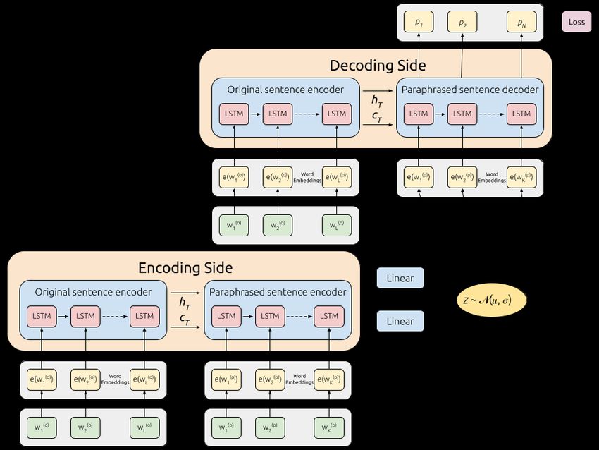
Gupta et al. [4] were the first to explore deep generative models for paraphrase
generation and proposed a model based on the Variational Auetoencoder
(VAE). The model is inspired by the text generation model proposed by
Bowman et al. [62] which is a VAE with the encoder and decoder being
modeled by LSTM networks. Gupta et al. customized the VAE-LSTM
architecture to fit paraphrase generation by introducing a module to both the
encoder and decoder to condition on the input sentence, which is shown
in Figure 3.1. This Conditional Variational Autoencoder (C-VAE) [63]
have previously been applied in computer vision tasks to generate images
conditioned on a given label, however it had not been applied in any NLP
tasks before.
The model were trained on data consisting of sentence pairs, containing
(o) (o) (o)
an original sentence denoted s(o) = {w1 , w2 , . . . , wn } and a paraphrased
(p) (p) (p)
sentence denoted s(p) = {w1 , w2 , . . . , wn }, respectively. The vector
representations of the sentences are denoted x(o) and x(p) and are learned using
LSTM networks with the rest of the model. The model can be divided into two
parts, the encoder model and the decoder model. The encoder side converts the
original sentence s(o) and feeds it through the first single-layer LSTM network
to produce its vector representation x(o) . The vector representation x(o) is then
fed along with the s(p) to produce the vector representation x(p) which then is
fed into two feed-forward neural networks to produce a mean and a variance
of the VAE encoder. The mean and variance are then used to sample a latent
variable z.
The decoder side of the network takes the latent variable z produced byYou can also read