Joint-instrument analyses with Gammapy - Master's Thesis in Physics - Friedrich-Alexander-Universität Erlangen ...
←
→
Page content transcription
If your browser does not render page correctly, please read the page content below
Joint-instrument analyses with
           Gammapy

    Master’s Thesis in Physics
                    Presented by

               Tim Unbehaun
             Date: 03. December 2020

      Erlangen Centre for Astroparticle Physics
           Friedrich-Alexander-Universität
                 Erlangen-Nürnberg

       Supervisor: Prof. Dr. Stefan Funk
   Co-advisor: Prof. Dr. Christopher van Eldik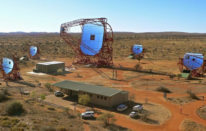
Contents
1. Introduction                                                                                                                                       6

2. Studying particle acceleration       with high energy γ-rays and neutrinos                                                                          8
   2.1 Multi messenger connection       . . . . . . . . . . . . . . . . . . . . . . . . .                                             .   .   .   .    8
       2.1.1 Leptonic interactions      . . . . . . . . . . . . . . . . . . . . . . . . .                                             .   .   .   .    9
       2.1.2 Hadronic interactions      . . . . . . . . . . . . . . . . . . . . . . . . .                                             .   .   .   .    9
   2.2 Relevant galactic sources . .    . . . . . . . . . . . . . . . . . . . . . . . . .                                             .   .   .   .   11
       2.2.1 The Crab nebula . .        . . . . . . . . . . . . . . . . . . . . . . . . .                                             .   .   .   .   11
       2.2.2 Vela X . . . . . . . .     . . . . . . . . . . . . . . . . . . . . . . . . .                                             .   .   .   .   12
       2.2.3 RX J1713.7−3946 . .        . . . . . . . . . . . . . . . . . . . . . . . . .                                             .   .   .   .   12

3. Instruments                                                                                                                                        13
   3.1 Imaging Air Cherenkov      Telescopes .    .   .   .   .   .   .   .   .   .   .   .   .   .   .   .   .   .   .   .   .   .   .   .   .   .   13
        3.1.1 H.E.S.S. . . . .    . . . . . . .   .   .   .   .   .   .   .   .   .   .   .   .   .   .   .   .   .   .   .   .   .   .   .   .   .   14
        3.1.2 CTA . . . . . .     . . . . . . .   .   .   .   .   .   .   .   .   .   .   .   .   .   .   .   .   .   .   .   .   .   .   .   .   .   14
   3.2 Fermi . . . . . . . . .    . . . . . . .   .   .   .   .   .   .   .   .   .   .   .   .   .   .   .   .   .   .   .   .   .   .   .   .   .   15
   3.3 KM3NeT . . . . . . .       . . . . . . .   .   .   .   .   .   .   .   .   .   .   .   .   .   .   .   .   .   .   .   .   .   .   .   .   .   16

4. Methodology                                                                                                                                        19
   4.1 The Gammapy package . . . . . . . . . . . . .                          .   .   .   .   .   .   .   .   .   .   .   .   .   .   .   .   .   .   19
   4.2 A Binned Maximum Likelihood Analysis . . . .                           .   .   .   .   .   .   .   .   .   .   .   .   .   .   .   .   .   .   20
   4.3 Likelihood Ratio Tests and confidence intervals                        .   .   .   .   .   .   .   .   .   .   .   .   .   .   .   .   .   .   21
   4.4 Pseudo Experiments . . . . . . . . . . . . . . .                       .   .   .   .   .   .   .   .   .   .   .   .   .   .   .   .   .   .   22
   4.5 NAIMA Models . . . . . . . . . . . . . . . . . .                       .   .   .   .   .   .   .   .   .   .   .   .   .   .   .   .   .   .   22

5. Combined KM3NeT - CTA analysis                                                                                                                     24
   5.1 Analysis preparations . . . . . . . . . . . . . . . . . . . . . . .                                    .   .   .   .   .   .   .   .   .   .   24
       5.1.1 Instrument response functions for KM3NeT . . . . . .                                             .   .   .   .   .   .   .   .   .   .   24
                5.1.1.1 Effective area . . . . . . . . . . . . . . . . . .                                    .   .   .   .   .   .   .   .   .   .   25
                5.1.1.2 Energy dispersion . . . . . . . . . . . . . . . .                                     .   .   .   .   .   .   .   .   .   .   25
                5.1.1.3 Point Spread Function . . . . . . . . . . . . .                                       .   .   .   .   .   .   .   .   .   .   28
       5.1.2 Background models for KM3NeT . . . . . . . . . . . .                                             .   .   .   .   .   .   .   .   .   .   28
                5.1.2.1 Atmospheric neutrino background . . . . . . .                                         .   .   .   .   .   .   .   .   .   .   29
                5.1.2.2 Atmospheric muon background . . . . . . . .                                           .   .   .   .   .   .   .   .   .   .   30
       5.1.3 Instrument response functions for CTA . . . . . . . . .                                          .   .   .   .   .   .   .   .   .   .   31
       5.1.4 Generation of the data sets . . . . . . . . . . . . . . .                                        .   .   .   .   .   .   .   .   .   .   32
   5.2 Initial results . . . . . . . . . . . . . . . . . . . . . . . . . . .                                  .   .   .   .   .   .   .   .   .   .   34
       5.2.1 Estimation of KM3NeT sensitivity . . . . . . . . . . .                                           .   .   .   .   .   .   .   .   .   .   34
       5.2.2 Test of a combined analysis on the Crab nebula . . . .                                           .   .   .   .   .   .   .   .   .   .   36
       5.2.3 Limits on the hadronic contribution . . . . . . . . . . .                                        .   .   .   .   .   .   .   .   .   .   38
   5.3 Updated results . . . . . . . . . . . . . . . . . . . . . . . . . .                                    .   .   .   .   .   .   .   .   .   .   41
       5.3.1 Optimization of quality cuts for the muon background                                             .   .   .   .   .   .   .   .   .   .   41
       5.3.2 Generation of new models . . . . . . . . . . . . . . . .                                         .   .   .   .   .   .   .   .   .   .   43
       5.3.3 Improved scan of the hadronic contribution . . . . . . .                                         .   .   .   .   .   .   .   .   .   .   43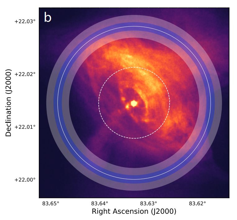
4

6. Combined analysis of H.E.S.S. and Fermi on the Crab nebula                                49
   6.1 H.E.S.S. data and comparison to the HAP analysis . . . . . . . . . . . . . . . . 49
   6.2 Fermi data and comparison to the Fermipy analysis . . . . . . . . . . . . . . . 53
   6.3 Combined analysis . . . . . . . . . . . . . . . . . . . . . . . . . . . . . . . . . . 54

7. Discussion & Conclusion                                                                  59

Appendices                                                                                  61

A. H.E.S.S. run lists                                                                       62

B. Parameters for H.E.S.S. seasons                                                          63

C. Neutrino selection cuts                                                                  64
5

.
6

                                                   Space is big. Really big. You won’t believe how
                                                   hugely mindboggling big it really is.

                                                     (Douglas Adams, “The Hitchhiker’s Guide to the
                                                                                           Galaxy”)

1.     Introduction
For as long as there are ancient recordings, humankind tried to figure out the true nature of
stars, the Sun and the moon in more or less scientific ways. Until rather recently only the
visible light could be used to gather information on stellar objects, some more nearby and
others very far away from the Earth. The mystery how stars generate their energy and light
was only solved after Albert Einstein’s theory of general relativity [Einstein, 1916] helped us
to understand gravity and stellar motions in a more fundamental way and after Quantum
mechanics were on its way. The young astronomer Cecilia Payne-Gaposchkin found evidence
for the high abundance of Hydrogen and Helium in the spectral absorption lines of stars in
1925. In her PhD thesis [Payne, 1925] she classified the results as “almost certainly not real”
because they were in contradiction to the current scientific consensus that stars are made of the
same materials as the Earth. Her results were confirmed a few years later by Arthur Stanley
Eddington leading to the model of nuclear fusion powering the stars. Today stellar physics is
able to describe most of the phenomena connected to stars very well. But stars are not the
only interesting objects in space and visible light is not the only messenger we can use to learn
about them. Various telescopes and observatories have helped to detect light ranging from radio
waves to γ-rays coming from rather exotic object classes hosting extreme conditions. Like this
we have discovered QUASARs and BLAZARs shining as bright as whole galaxies and Super
Novas and Gamma Ray Bursts with enormous explosion energies and many more. Even though
we have some ideas how some of these sources are able to accelerate charged particles up to
energies in the order of 1021 eV [Becker, 2008], there are a lot of open questions, e.g. which kind
of charged particles are dominantly accelerated for each source class and which spectral shape
do they follow. Until now most analyses on these sources are based on observations by one
telescope or detector only considering the energy range or particle type accessible to it. Like
this great progress has been made in detecting and characterizing thousands of (extra-)galactic
particle accelerators. In order to learn even more about them the next step is to take the whole
picture into consideration and to combine the measurements of different instruments. Even
though combined analyses of different instruments have been performed before e.g. by taking
published flux points of a source in different energy ranges, it seems much more promising to
combine the lower level data of the instruments. In this way one can simultaneously fit the
spatial morphology and the spectral shape of one source seen by multiple different instruments
and calculate the correlation between the free parameters. One can also directly fit physical
models predicting γ-ray and neutrino fluxes to the data of the respective instruments and
link the physically connected parameters. This is especially interesting because both γ-rays
and neutrinos can be produced by the same hadronic interactions at the source leading to a
multi-messenger connection. This would mean that if one source is accelerating e.g. protons
and other hadronic particles and the γ-ray emission is caused by these particles one would also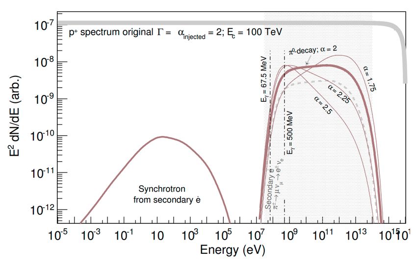
1 Introduction                                                                                  7

expect a flux of neutrinos coming from that source. Even though the neutrino telescope IceCube
has successfully measured a diffuse galactic neutrino flux, until now only one neutrino event
could be associated with one individual source at the 3σ level. This event had a most likely
energy of 290 TeV and was detected in coincidence with a flaring BLAZAR in September 2017
[Williams, 2019]. In order to exploit the multi-messenger connection in such combined analyses
one would need publicly available data of the instruments which will be the case for the currently
in building phase Cherenkov Telescope Array (CTA) and the next generation neutrino detector
KM3NeT. One also needs a suitable software package able to read and analyse data from both
instruments which are also currently in development. One example is Gammapy which is an
open-source Python package designed for gamma-ray astronomy but also able to analyse data
from different instruments (e.g. neutrino data) once the instrument data is available.
In the first part of this thesis a combined analysis of CTA and KM3NeT data with Gammapy
will be simulated and constraints on the production mechanisms for leptonic and hadronic
emission scenarios will be calculated. While CTA will measure γ-rays in an energy range from
20 GeV up to over 100 TeV, KM3NeT will be sensitive to neutrinos in a range from 100 GeV
up to 100 PeV. With its location on the northern Hemisphere it can observe a large fraction
of the galactic disc including many interesting galactic sources. This kind of analysis might
help in the future to improve the understanding of certain galactic γ-ray sources regarding their
acceleration mechanisms.
The second part of this work will be about a combined analysis of H.E.S.S. and Fermi LAT data
on the Crab nebula also using Gammapy. Fermi is a space based γ-ray telescope with an energy
range of ∼20 MeV to ∼1 TeV and H.E.S.S. is a ground based Imaging Air Cherenkov Telescope
measuring γ-rays in a range from ∼50 GeV to 100 TeV. Both instruments have observed the
Crab nebula which is the brightest, steady TeV γ-ray source. It is very well studied and the
perfect candidate to test a combined analysis of different instrument data using Gammapy.
The goal here is to compare the Gammapy analyses of H.E.S.S. and Fermi data to the analyses
performed with standard analysis tools and to check for consistency. Once this is ensured the
combination of the data will extend the energy ranges of the individual instruments and a
physically motivated model can be fitted to the data. Furthermore it is interesting to determine
the Crab’s extension in different energy bands. It would be the first time that this is done in a
consistent way over this extended energy range measured by different instruments.
8
We have already discovered the basic laws that
govern matter and understand all the normal
situations. We don’t know how the laws fit together,
and what happens under extreme conditions.
(Stephen W. Hawking)
2. Studying particle acceleration with high energy γ-rays
and neutrinos
This section will give an overview of the connection between high energy γ-rays and neutrinos
and their production mechanisms at astrophysical sources. The energies of these particles exceed
the energies accessible in particle accelerators at Earth by far. By observing these sources and
learning about production and acceleration mechanisms we can test physical models in the limit
of very high energies and extreme conditions.
2.1 Multi messenger connection
The Earth is exposed to a continuous flux of charged particles from space, called cosmic rays
(CR), in a wide range of energies. This was already discovered by Viktor Hess in 1912 with his
balloon flights [Hess, 1912]. He could show that the abundance of ionizing particles increases
with increasing distance to the ground, indicating that the flux was not coming from radioactive
solids in the ground. Today we believe that galactic and extra-galactic sources are accelerating
charged particles to very high energies (up to ∼ 1021 eV) [Becker (2008, chapter 3.1.1.1)]. Known
acceleration mechanism are e.g. the one-shot acceleration where a particle gains energy in a
continuous way from an ordered field or the Fermi shock acceleration. Here particles gain their
energy successively when passing a shock front over and over again while being confined in
the shock region by magnetic fields (for more detail see e.g. Bustamante et al. (2010)). The
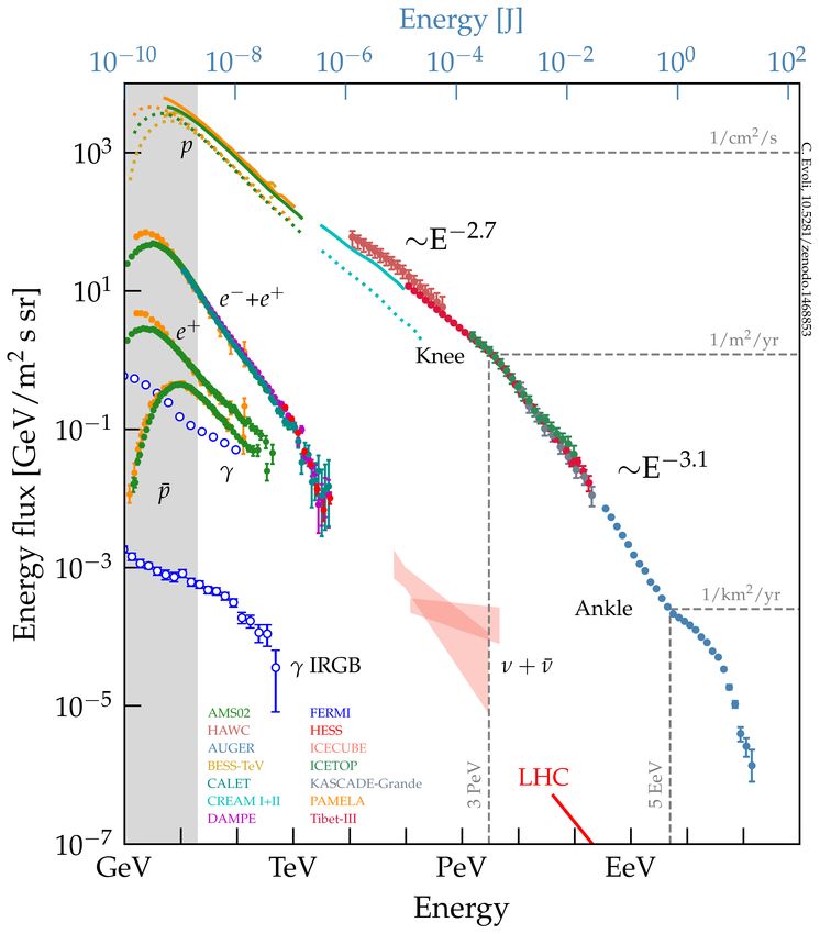
CR spectrum measured at Earth is shown in figure 1 (left) and follows a steep power-law. It
consists mostly of protons (∼90%) and heavier nuclei where the exact composition is energy
dependent. Electrons and positrons only make up for about 1% of the cosmic rays. If we want
to learn more about the acceleration mechanisms inside one particular source one cannot simply
measure the CR spectrum from the source’s direction since charged particles are deflected by the
galactic magnetic fields, so they do not point back. This is at least the case for CR with energies
ECR < Z · 1017 eV. Above this energy the flux of CR is very low due to its steep power-law
spectrum so it is difficult to gather enough statistics on these very high energy events from one
source. An alternative way to study (extra-)galactic particle accelerators is to look at neutral
particles emitted by them. Even though neutral particles cannot be accelerated directly by
electric fields or the Fermi acceleration mechanisms, they are produced in particle interactions
of high energy CR in the source’s vicinity. Dependent on the kind of the interaction (hadronic
or leptonic) high energy neutrinos and/or high energy photons are produced. These neutral
particles point back to their sources and by measuring their spectrum we can draw conclusions
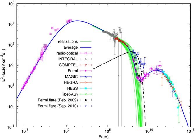
on the primary particle population. The spectrum of the messenger particles measured at Earth
can be seen in figure 1 right.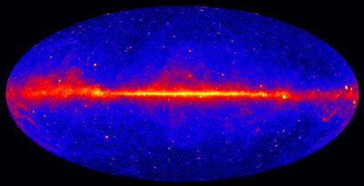
2 Studying particle acceleration with high energy γ-rays and neutrinos 9
Figure 1: Left: Cosmic ray spectrum measured by different experiments (see legend). Also
shown is the composition of the spectrum for the lower energies [Evoli, 2018]. Right: Spectrum
of the multi-messenger particles. The diffuse γ-ray background measured by Fermi (red) is
compared to the neutrino flux measured with IceCube (black) and the cosmic ray flux (green)
measured with the Pierre Auger observatory [Murase and Waxman, 2016].
2.1.1 Leptonic interactions
Typical sources that produce their γ-ray emission to a large extent in leptonic interactions are
pulsars and pulsar wind nebulae. Those sources accelerate electrons and positrons to very high
energies. These can than emit Synchrotron radiation in possibly present magnetic fields and thus
produce γ-rays up to a theoretical maximal energy of Eγ = κ · 68 MeV with κ = 1 − 3 [Aharonian
et al., 2004]. So the Synchrotron component is not responsible for the high energy γ-rays above
1 GeV. These can be produced when the very high energy e− /e+ directly transfer their energy
to low energy photons present in so-called seed photon fields through the Inverse Compton
scattering process (IC). The seed photon fields can be the Cosmic Microwave Background
(CMB), far-infrared dust emission (FIR), near-infrared stellar emission (NIR) or the Synchrotron
photon field (SSC) produced by the same electrons/positrons. The characteristic shape of the
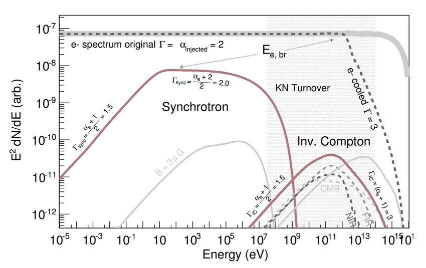
Synchrotron and Inverse Compton flux resulting from an electron spectrum can be seen in
figure 2 (Top). In contrast to hadronic interactions there are no neutrinos produced in leptonic
interactions.
2.1.2 Hadronic interactions
Typical sources which might feature a hadronic γ-ray production are Super Novas and their
remnants or Active Galactic Nuclei. In hadronic interaction both photons and neutrinos can be
produced. The conventional models consider high energy protons interacting with low energy
protons or matter fields in or around the acceleration region. In these interactions π + , π − , π 0 are
produced with about equal abundances (as well as other interaction products). The neutral pions
decay mostly into two photons while the charged ones decay into leptons and their corresponding
neutrino
π 0 −→ γ + γ (2.1)
(−) (−)
π ± −→ µ± + ν µ −→ e± + νµ + ν̄µ + ν e (2.2)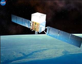
10

Figure 2: Top: Spectral energy distribution of an electron spectrum (light gray) and the
resulting Synchrotron and Inverse Compton flux (brown). Bottom: Spectral energy distribution
of a proton spectrum (light gray) and the resulting γ-ray spectrum from Pion Decay (brown)
[Funk, 2015].

For the charged pion decay the electron channel is strongly suppressed because of helicity
conservation. In figure 3 the Feynman diagrams for these interactions are shown. The average
energy transferred to one pion in a pp-interaction is about 0.2 · Ep and is rather independent on
the protons energy. The four leptons resulting from a π ± decay will approximately carry the
same amount of energy, which means that the neutrinos produced in pp-interactions have an
energy Eν ≈ Ep /20 [Becker, 2008]. Similar the two γ-rays will have an energy of Eγ ≈ Ep /10.
This means that the shape of the neutrino and γ-ray spectrum is close to the proton spectrum
which is just shifted in energy, at least well above the mass scale of the π 0 of 135 MeV. The
γ-ray emission from an exemplary proton spectrum can be seen in figure 2 (bottom).
2 Studying particle acceleration with high energy γ-rays and neutrinos                           11

                            γ                                                        νµ
                                                               +
                                                           µ
                                                                                            νe
           u                              d                         µ−
      π0              u              π+
           u                              u          W+                      W−

                                                           νµ
                            γ                                                               e−
               (a)                                   (b)                     (c)
Figure 3: Feynman diagrams of the neutral pion decay (a), the charged pion decay on the
example of the π + (b) and the muon decay (c).

If we don’t distinguish between neutrinos and anit-neutrinos1 the ratio of (νe : νµ : ντ ) for pion
decay is (1 : 2 : 0) according to equation 2.2. Due to neutrino oscillation the expected ratio at
Earth is (1 : 1 : 1) when the source is outside the solar system [Becker, 2008].

2.2        Relevant galactic sources
In the following an overview of the three relevant sources analysed or simulated in the thesis is
given: RX J1713.7−3946, Vela X and the Crab nebula.

2.2.1      The Crab nebula

The Crab nebula is the brightest steady source of TeV γ-rays. In 1054 Chinese astronomers
reported a bright explosion event not knowing that it corresponded to a core-collapse supernova
in the constellation of Taurus about 2 kpc away from Earth. After the supernova a fast rotating
neutron star was left behind which powers an outflow of highly relativistic particles with its
rotational energy losses. Today’s best models assume that this outflow consists of mostly electrons
and positrons which get further accelerated in the termination shock about 0.5 light years (ly)
away from the pulsar. These electrons/positrons can reach energies up to 1015 eV filling the
area of about 10 ly in diameter after the termination shock. They emit Synchrotron radiation in
the ambient magnetic fields, producing the low energy part of the spectrum in figure 4 up to
∼1 GeV. The high energy part of the spectrum is produced by Inverse Compton up-scattering of
low energy photons by the same electrons/positrons [Abdalla et al., 2019]. This whole system
is now called the Crab pulsar wind nebula (PWN) with its morphology (in X-rays) shown in
figure 4 (right panel) with the bright pulsar in the center followed by the termination shock and
the region of non-thermal particle wind.
Detailed multi-wavelength analyses of the spectrum have been performed e.g. by Yuan et al.
(2011) and Meyer et al. (2010) fitting a physical model to the electromagnetic emission of the
Crab nebula. These studies show that the emission from radio energies up to γ-ray energies
can be reasonable well described by the model. There is also a strong evidence for an energy
dependent extension of the Crab nebula at γ-ray energies. Fitting the extension in several
energy bands which was done by Yeung and Horns (2019) shows that the extension decreases
towards higher energies. Since the γ-rays from different energy bands can be associated with
primary electrons of different energies, it means that we can learn about the propagation of
very high energy (VHE) electrons in the Crab’s vicinity.

 1
     neutrino detectors like KM3NeT cannot do this
12 Figure 4: Left: Spectral energy distribution of the Crab nebula from radio waves to γ-rays. The lines show fits to the data points measured by the instruments listed in the legend. For details see Yuan et al. (2011). Right: Chandra X-ray image (courtesy of M. C. Weisskopf and J. J. Kolodziejczak). The H.E.S.S. extension is shown as solid white circle overlaid on top of shaded annuli indicating the statistical and systematic uncertainties. The Chandra extension, corresponding to 39% of the X-ray photons, is given as dashed white circle. Taken from Abdalla et al. (2019). 2.2.2 Vela X Vela X is one of the nearest pulsar wind nebulae at a distance of about 0.29 kpc [Abramowski et al., 2012] and is associated with the energetic Vela pulsar PSR B0833-45. Similar to the Crab nebula most models assume a leptonic generation of the VHE γ-rays. None the less it is not clear to what extent also protons contribute to the total γ-ray flux from Vela X. In order to put strong constraints of the hadronic fraction it might be helpful to look for (the lack of) neutrinos coming from that source. 2.2.3 RX J1713.7−3946 RX J1713.7−3946 is a young shell-type Super Nova Remnant (SNR) which is located at a distance of about 1 kpc. In its shock front charged particles are accelerated to very high energies which also cause γ-ray emission that we can observe at Earth. The origin of the γ-ray emission extending up to about 100 TeV is still unclear. In the latest H.E.S.S. paper [Abdalla et al., 2018] on RX J1713.7−3946 both leptonic and hadronic models have been fitted to the combination of H.E.S.S. and Fermi LAT data where neither model could be accepted unambiguously. However molecular clouds in the vicinity of the source could be an indication for a hadronic production mechanism.
3 Instruments                                                                                    13

                                                  An experiment is a question which science poses to
                                                  Nature, and a measurement is the recording of
                                                  Nature’s answer

                                                     (Max Planck, “The Meaning and Limits of Exact
                                                                                         Science”)

3.     Instruments
The following section gives an overview of the four relevant instruments in this thesis. Beginning
with the ground-based Imaging Air Cherenkov telescopes (IACTs) H.E.S.S. and CTA which can
detect γ-rays between ∼50 GeV and 100 TeV. The lower energy γ-rays in a range from ∼20 MeV
to ∼1 TeV can be detected with the Fermi satellite. The currently in building phase next level
neutrino detector KM3NeT will be able to detect neutrinos in an energy range from 100 GeV up
to 100 PeV.

3.1    Imaging Air Cherenkov Telescopes
IACTs collect the Cherenkov light of particle showers. These air showers are produced by high
energy primary particles (γ-rays or CR) when they enter the Earth’s atmosphere at an altitude
of about 20 km. There are electromagnetic cascades (fig. 5a) consisting of electrons, positrons
and γ-rays. The dominant processes are pair production and Bremsstrahlung which happen
consecutively until the secondary particles are below a critical energy. The number of secondary
particles is proportional to the energy of the primary particle and the altitude of the shower
maximum depends logarithmically on the energy of the primary γ-ray (∼10 km AMSL for
Eγ = 1 TeV) [Funk, 2015]. The opening angles of the leptonic interactions are small (typically
< 1◦ ) and the Molière Radius (radius that contains 90% of the particles) is around 90 m.
There are also hadronic showers induced by protons or heavier nuclei (fig. 5b). In these showers
Mesons like pions are produced in hadronic interactions which then decay into two γ-rays or
muons and muon neutrinos. The γ-rays or the electrons from the muon decay then produce
electromagnetic sub-showers. The hadronic interactions give proton showers larger transverse
momentum and make them more irregular. The difference in shape and composition compared
to electromagnetic showers can be used to suppress the hadronic background which dominates
the γ-ray signal by a factor of up to 104 .
The Cherenkov light cones are produced when charged particles travel through a dielectric
medium faster than the speed of light in that medium. The medium is electrically polarized
along the track and is emitting electromagnetic waves that do not interact destructively as
it would be the case for slower particles. Figure 5c shows the Cherenkov light pool with an
diameter of about 240 m at the ground. However for a typical shower there are only ∼100
photons per m2 and TeV arriving at the ground in good atmospheric conditions [Funk, 2015].
Even though these Cherenkov light flashes are very faint they can still be detected over the
night sky background light by high time resolution cameras. Almost all of the Cherenkov
photons arrive at the ground within a few nanoseconds, a very short time frame in which
only few background photons arrive. The cameras consist of an array of Photo multipliers
14
Figure 5: Illustration of a) Electromagnetic cascade with pair production and Bremsstrahlung,
b) Hadronic air shower induced by a proton with electromagnetic sub-showers, c) Air shower
with the resulting Cherenkov light cone (images from a presentation by Daniela Dorner, 2019).
(PMTs) each representing one pixel. When multiple PMTs surpass a threshold an image of the
shower is recorded. With a reconstruction algorithm the energy, direction and shower type can
be determined. The reconstruction improves when using a stereoscopic system with multiple
telescopes looking at the same shower. This is done in the H.E.S.S. experiment and will also be
used in the Cherenkov Telescope Array (CTA).
The advantage of this method is that the big area of the atmosphere can be used to detect
the low γ-ray fluxes in the TeV range. The draw back is that IACTs can only operate in dark,
moonless nights without clouds. Furthermore since the atmosphere is part of the detector it can
not be calibrated directly, instead Monte Carlo simulations are used for that.
3.1.1 H.E.S.S.
The High Energy Stereoscopic System (H.E.S.S.)2 is located in Namibia, near the Gamsberg
mountain at an altitude of 1800 m (compare figure 6). Phase I consists of 4 telescopes each
with 108 m2 mirror area positioned at the corners of a square with 120 m side length. All four
telescopes were operational in December 2003. In Phase II a bigger telescope with 614 m2 mirror
area was added in the center of the array to improve the angular resolution and measure to even
lower energies. It started operation in July 2012. In 2016 the cameras and light collimators of
the original HESS-I array have been exchanged. Observations with the new cameras belong to
the so-called HESS-IU season.
3.1.2 CTA
The Cherenkov Telescope Array3 will be the next generation IACT. It will consist of two sites,
one at the northern hemisphere in La Palma and one at the southern hemisphere in Chile.
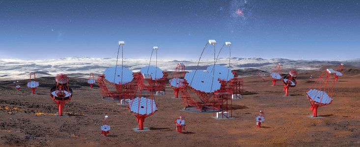
Together both sites will have more than 100 telescopes in three different sizes (compare figure 7).
There are 70 Small-Sized Telescopes (SSTs) planned with an mirror area of 8 m2 and 10.5◦ field
of view measuring energies from a few TeV up to 300 TeV. All of the SSTs will be located at the
southern observatory. The Medium-Sized Telescopes (MSTs) will be built in different versions.
2
https://www.mpi-hd.mpg.de/hfm/HESS/
3
https://www.cta-observatory.org3 Instruments 15
Figure 6: Photo of the five H.E.S.S. telescopes. Credit: H.E.S.S. collaboration.
One will use a modified Davies-Cotton optical design and use FlashCam and NectarCam4 based
on PMTs. The effective mirror area is 88 m2 and the pixel size corresponds to 0.17◦ . The
alternative version uses the dual mirrored Schwarzschild-Couder optical design for better light
focus and imaging details. It only uses 41 m2 of effective mirror area and its camera based
on silicon photo multipliers with >11 000 pixel (0.067◦ pixel size) is designed to improve the
shower reconstruction. Fifteen of the MSTs will be located at the northern observatory and
25 at the southern. Each site will also have four Large-Sized Telescopes (LSTs) with parabolic
optical design and 370 m2 of effective mirror area to measure γ-rays down to 20 GeV. CTA is
expected to be ten times more sensitive than existing experiments and offer better angular
and energy reconstruction of the events. The measured data will be publicly available which
makes combined analyses with other instruments possible. The beginning of the observatory
observations is planned for 2022 and the construction project should be completed in 2025.
3.2 Fermi
The Fermi Gamma-ray Space Telescope 5 was launched on June 11, 2008 by NASA. The satellite
is hosting two instruments as can be seen in figure 8 left: The Large Area Telescope (LAT)
and the Gamma-ray Burst Monitor (GBM), where only the LAT is relevant for this work. The
LAT is a pair-conversion telescope with a precision converter-tracker and calorimeter. Since
high energy γ-rays cannot be deflected or refracted the detection principle of the LAT is based
on the e+ /e− pair production when γ-rays interact with the satellite. The converter-tracker
consists of 16 planes of high-Z material (wolfram) offering an increased cross section for the
pair production. The direction of the charged particles is measured with position-sensitive
detectors. The calorimeter serves two purposes. First measuring the energy of the particle
shower induced by the γ-ray and second imaging the shower development profile which can be
used as a background discriminator [Atwood et al., 2009]. Each calorimeter module consists of
4
https://www.cta-observatory.org/project/technology/mst/
5
https://fermi.gsfc.nasa.gov/16
Figure 7: All three telescope classes planned for the southern CTA observatory. Credit:
CTA/M-A. Besel/IAC (G.P. Diaz)/ESO
96 CsI(Tl) crystals optically isolated from each other. Furthermore the anticoincidence detector
provides charged particle background rejection. There are 89 scintillation plates surrounding the
converter-tracker which detect incoming charged particles with an efficiency of 0.9997 averaged
over the detector volume. The LAT detector could be calibrated before the launch offering an
energy resolution ∆E/E of +5% - 10%. The angular resolution improves from 3.5◦ at 100 MeV
to ≤0.15◦ at ≥ 10 GeV. Figure 8 right shows the all-sky map recorded with the LAT. The source
catalog 4FGL-DR2 contains 5788 entries and is based on 10 years of LAT observation [Abdollahi
et al., 2020]. Since the γ-ray flux is following a steep power-law for most sources the detection
area of Fermi LAT is not big enough to gather enough statistics above ∼300 GeV. It is also not
affordable to send larger instruments into space, that is why ground-based detectors are used
for the higher energies.
Figure 8: Left: An artist’s drawing of the Fermi-satellite orbiting Earth. The LAT can be seen
on top of the GBM (Credits: NASA E/PO, Sonoma State University, Aurore Simonnet). Right:
Gamma-ray all-sky map for energies greater than 1 GeV based on 5 years of LAT observation
(Credit: NASA/DOE/Fermi LAT Collaboration).
3.3 KM3NeT
The IceCube neutrino observatory6 is detecting high energy neutrinos in the antarctic ice since
2010. It could measure a diffuse astrophysical neutrino flux but only very few neutrinos could
6
https://icecube.wisc.edu/3 Instruments 17
be assigned to individual sources, none of them in our galaxy [Williams, 2019]. Because of its
location on the south pole it can only observe a limited fraction of the galactic sources through
the Earth which is an important filter for the atmospheric muon background.
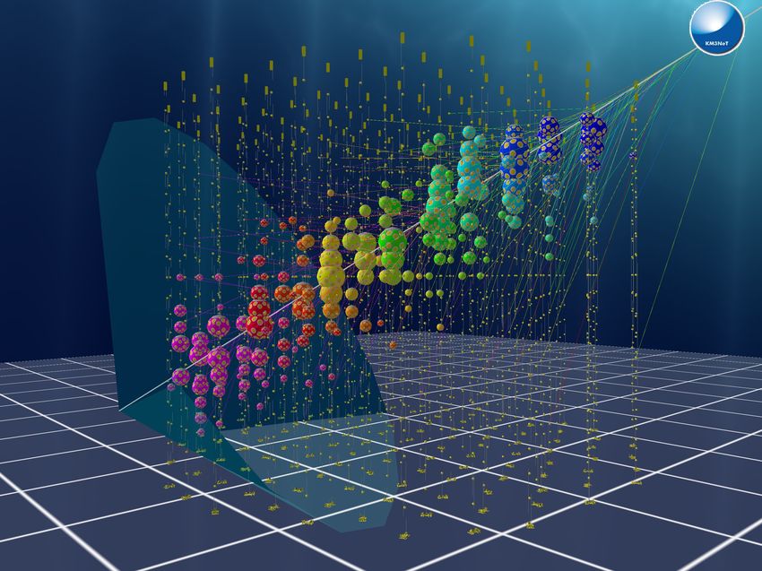
KM3NeT7 is a project for the next generation neutrino telescopes located in the Mediterranean
Sea. The ARCA (short for Astroparticle Research with Cosmics in the Abyss) telescope will
look for neutrinos from distant astrophysical sources such as supernovae, gamma ray bursters
or colliding stars. The ORCA telescope will be used to study neutrino properties exploiting
neutrinos generated in the Earth’s atmosphere. ARCA will be mapping 87% of the sky including
most of the galaxy and the galactic center. Because of its location on the northern hemisphere
(36°16’ N 16°06’ E) sources on the southern hemisphere can be observed through the Earth
filtering the atmospheric muon background. ARCA phase 2.0 will consist of two detector blocks,
each made of 115 KM3NeT vertical detection units which are anchored in 3500 m depth. Each
detection unit is about 700 m in height and connects 18 optical sensor modules with about 40 m
distance in between (compare figure 10). The detection units will be placed about 100 m apart,
instrumenting a volume of about 1 cubic kilometer which is slightly larger than IceCube. The
optical sensor modules (DOMs) are glass vessels with 31 photo multiplier tubes looking in all
direction to detect the Cherenkov light from the charged particles that are produced in neutrino
interactions. The ORCA array will be optimised for the lower neutrino energies necessary for
the measurement of the neutrino mass hierarchy and thus instrumented more densely but will
also be 250 times smaller than ARCA.
The detection principle of neutrino detectors is based on neutrino interactions with nucleons of
the water via deep inelastic scattering. Since neutrinos are only interacting weakly there are
charged current (CC) and neutral current (NC) interactions of which the Feynman diagrams
are shown in figure 9. The four different scenarios all produce different signals in the detector
Figure 9: Feynman diagrams of the neutrino interaction channels visible to neutrino telescopes.
A neutral current reaction resulting in a hadronic cascade and an invisible outgoing neutrino
is shown in (a). Electron neutrinos reacting via the charged current yield an electron that
immediately showers and forms an electromagnetic cascade overlaid to the hadronic one (b).
Production of muons via CC is shown in (c), whereas (d) shows the reaction of tau neutrinos
and the eventual decay of the τ into a hadronic cascade. Taken from Kopper (2010).
which collects the Cherenkov light emitted by the charged particles produced in the interaction
(compare figure 10 right panel). The NC interactions happening through the exchange of a
Z0 -boson look the same in the detector independent of the incoming neutrino flavour. A hadronic
cascade is initiated at the interaction point which is seen by the detector but not containing all
the energy of the primary neutrino since it is leaving the detector again with some of its initial
energy. CC interactions with the exchange of a W± -boson produce a lepton of the neutrino
7
https://www.km3net.org/18 Figure 10: Left: Visualization of the KM3NeT array with a zoom on the optical sensors and the Cherenkov light cone from an incident muon event. Right: Simulation of an neutrino event seen by the KM3NeT detector. The color denotes the timing information and the size of the DOMs the amount of light registered (Credit: KM3NeT). flavour in addition to the hadronic cascade. In case of a νe the resulting electron will initiate an electromagnetic cascade overlaying the hadronic one. Both cascades contain the whole energy of the incoming neutrino which is good for the energy resolution of such events. A muon produced in a νµ interaction can have path lengths in water ranging from a few meters at GeV energies up to a several kilometers at a few TeV. This means that for high energy muons seen by the detector it is very likely that their vertex is outside the detector which increases the effective detector volume over the actually instrumented one but makes it hard to achieve a good energy resolution. Below energies of ∼10 TeV the angular resolution of muon tracks is limited by the neutrino interaction kinematics. For higher energies the angle between the neutrino direction and the muon direction becomes very small which allows for the best angular resolution of all the event types because of the long lever arm of the muon tracks. For ντ events the initial hadronic cascade is followed by a second one when the tauon decays. Both cascades can be detected separately if the distance between them is large enough. These events are also called double bang events [Kopper, 2010]. Based on these detection methods neutrino telescopes can not distinguish between neutrinos and anti-neutrinos. For this analysis only muon neutrinos will be considered since both the angular resolution as well as the effective area for muon events are superior to those of electron or tauon events. Currently ARCA is running in a starting phase with one string. After completion the data will be publicly available with a delay time of two years. The IRFs should be available by next year already.
4 Methodology                                                                                           19

                                                        A mathematical truth is timeless, it does not come
                                                        into being when we discover it. Yet its discovery is
                                                        a very real event, it may be an emotion like a great
                                                        gift from a fairy.

                                                                                       (Erwin Schrödinger)

4.       Methodology
4.1       The Gammapy package
Gammapy8 is an open-source Python package primarily developed for the analysis of IACT
data. It is based on existing Python packages like numpy, scipy and astropy. Even though
it is a prototype for the CTA science tools it can also be used to analyse data from different
instruments if the necessary instrument response functions (IRFs) are given. During the writing
of this thesis Gammapy is still in development and the latest stable version (v0.17) is used for
all the relevant analyses.
Gammapy features one dimensional spectral analyses, temporal analyses by calculating the
light curve and three dimensional analyses with one spectral and two spatial dimensions of
the given observations. Only the latter is relevant for this work and will be discussed here.
The IRFs, measured counts, background model and source model(s) are all combined in the
MapDataset class. The information of the reduced data and IRFs is stored in WcsNDMap classes.
The data is stored in a ND numpy array together with an WcsGeom object which holds the
information about the pixel coordinates and the axes of the map. For more information on the
implementation of the IRFs in Gammapy see section 5.1.1.

There are various built-in spectral and spatial models within Gammapy. The spectral models
return a flux Φ(E) dependent on the energy E and the spectral parameters. Relevant for this
thesis are the power-law model parameterizing the flux in the following way
                                                                −Γ
                                                            E
                                     Φ(E) = A ·                                                       (4.1)
                                                            E0

and the exponential-cutoff power-law model
                                                 −Γ      "       β #
                                             E                  E
                            Φ(E) = A ·                  exp −                                         (4.2)
                                             E0                Ecut

with A the amplitude, E0 the reference energy, Γ the spectral index, Ecut the cutoff energy and
β the cutoff exponent. There is also the Log Parabola model
                                                       −α−β log(E/E0 )
                                                  E
                                Φ(E) = A ·                                                            (4.3)
                                                  E0
 8
     https://gammapy.org
20
where β describes the curvature of the model. Also important for this work is the
NaimaSpectralModel class which takes a NAIMA radiative model as argument and returns
the flux predicted by it. For more detail see section 4.5.
The spatial models return the flux dependent on the sky coordinates and other parameters. The
simplest model is the Point spatial model where all of the flux is assigned to just one pixel if
the source position is also centered on that pixel. Else the flux is re-distributed across the four
neighbouring pixels to ensure the center of mass position is conserved. For extended sources
one can use the Disk spatial model which distributes the flux in a disk with radius r0 in a way
that the flux inside the disk is constant and outside zero. Or the Gaussian spatial model which
distributes the flux according to a Gaussian
1 − cos θ
Φ(θ) = N × exp −0.5 · (4.4)
1 − cos σ
where N is the normalization, θ is the sky separation to the model center and σ is the extension
of the model. Both the Disk and Gaussian model are normalized so that the total flux of the
model is conserved. They can also be elongated with an eccentricity and rotation angle.
The spectral and spatial models are combined in the SkyModel class which then returns the
model flux dependent on the energy and the spatial coordinates.
For the analysis a binned maximum likelihood method is implemented. The source models are
evaluated on the geometry of the exposure map which gives a number of predicted counts for
each pixel. The energy axis of the exposure map is defined in true energy, the spatial axes are
the same as for the counts map. The predicted-counts map is then forward folded with the
Energy Dispersion matrix for the energy dimension and with the Point Spread Function for the
spatial dimensions. After that the predicted-counts map is given in reconstructed energy which
is the same as for the counts map. True and reconstructed energy can differ in e.g. the number
of bins per decade so the model can be evaluated in a finer energy binning which increases the
precision. The background model is already defined on the counts geometry and simply holds
the number of predicted background counts for the live time of the data set. It can be scaled
using its norm parameter and tilted in the energy dimension. After all models are evaluated the
resulting maps are stacked which gives the total number of predicted counts in each pixel for
the respective model parameters.
For each MapDataset one can set masks, the mask_safe defining the safe data range and the
mask_fit defining the data range used for the Fit. The Fit class takes a list of data sets
and only considers pixels where both masks are True. It offers different fitting backends like
“minuit” 9 , “sherpa” 10 or “scipy” 11 to maximize the agreement between the model and data by
variation of the free model parameters.
4.2 A Binned Maximum Likelihood Analysis
The test statistic or TS-value is a measure for the agreement between the experimental data and
the model prediction. An ideal model would predict exactly the number of measured counts in
each pixel, however a realistic analysis will always show some discrepancies or residuals between
the measured data and the predicted one. In order to find the model most likely to best describe
9
https://iminuit.readthedocs.io/en/stable/index.html
10
https://cxc.cfa.harvard.edu/sherpa4.12/
11
https://docs.scipy.org/doc/scipy/reference/generated/scipy.optimize.minimize.html4 Methodology 21
the data, the likelihood L(ξ) for a set of model parameters ξ is computed in the following way
N
Y
L(ξ) = P(ni |νi (ξ)) (4.5)
i=1
with
νini (ξ)
P(ni |νi (ξ)) = · exp(−νi (ξ)) (4.6)
ni !
being the Poisson probability to measure ni events given the model prediction νi (ξ) in the pixel
i. The TS-value is defined as
N ni
X νi (ξ)
T S ≡ −2 ln L(ξ) = −2 ln · exp(−νi (ξ)) (4.7)
i=1
n i !
If one wants to find the parameter values that fit the measured data best one has to maximize
L or minimize the TS-value [Tanabashi et al. (2018, chapter 39.2.2)][Mohrmann, 2015].
The parameters can be confined into a physically reasonable range using hard boundaries which
the parameters can not exceed at all, or by using penalty terms which add contributions to the
total TS-value for deviations from some central values ξ ∗ . While the hard boundaries correspond
to a box-potential where the parameter can move freely inside, the so-called prior functions can
describe any kind of potential. Often times one would use a set of Gaussian-shaped functions
which then add contributions to the TS-value in the following way
N
νini (ξ) ∗ 2
X
X (ξm − ξm )
T S = −2 ln · exp(−νi (ξ)) + 2
(4.8)
i=1
ni ! m
∆ξm
where one can control the width of the potential for each parameter ξm by adjusting ∆ξm . This
approach can also be used when one needs to constrain quantities during the fit that are not
free parameters of the fit itself. One example could be to confine the ratio of two models during
the fit.
4.3 Likelihood Ratio Tests and confidence intervals
If one wants to compute the level of agreement of two models M1 and M2 to some measured
data one can use the ∆TS-value.
∆T S = T SM1 − T SM2 = −2 ln(LM1 /LM2 ) (4.9)
Wilk’s theorem states that if the two models are nested, e.g. the parameter space of M1 is a
subset the parameter space of M2 and the sample size is sufficiently large and no parameter
value is close to a physical bound, then the ∆TS-value is χ2 distributed with k degrees of
freedom, where k is the difference in number of free parameters between M1 and M2 [Wilks,
1938],[Mohrmann, 2015]. In this case the square root of the ∆TS-value corresponds to the
significance with which M2 is preferred over M1.
If one the conditions above is not full filled one might not want to trust Wilk’s theorem but
instead use the more general Bayesian approach. Here the probability which indicates how much
more likely M2 is compared to M1 can be calculated by solving equation 4.9 for the likelihood
ratio.
LM 1 1
= e− 2 ∆T S (4.10)
LM 222
In order to obtain confidence intervals for one parameter, a so-called profile likelihood scan is
carried out. The parameter of interest is fixed to a set of values in a range around its best-fit
value and the TS-values are calculated and compared to the TS-value without this constraint.
If the ∆TS-values follow a parabola when plotted over the scanned parameter values then
it is χ2 -distributed and the confidence intervals follow analogously. If this is not the case a
∆TS-value does not directly correspond to a confidence interval but one can still use equation
4.10 to compute the probability density function (p.d.f) for the parameter values. Then one can
look for the parameter values for which the integral over the p.d.f contains e.g. 90% of its area
in order to obtain the 90% confidence interval.
4.4 Pseudo Experiments
Knowing the Instrument Response Functions of an instrument one can simulate measured data
even if the instrument is not built yet. Like this one can estimate its sensitivity to certain source
models. There are two possibilities to do that.
The first is to draw Poisson randomized counts based on the model prediction for each pixel.
The drawback of this method is that one needs a sufficiently large number of these pseudo
experiments in order to average over statistical fluctuations.
The second possibility is to use the so-called Asimov data set. Here the counts cube is exactly
the predicted counts cube without any randomization. Hence a minimization of the TS-value
would will return the input parameters. Cowan et al. (2011) have shown that this data set is a
representative data set for the assumed model prediction without the statistical fluctuations of
the first method. So it can also be used to estimate the expected sensitivity of the experiment.
4.5 NAIMA Models
NAIMA12 is a Python package for computation of non-thermal radiation from relativistic particle
populations. Gammapy has a wrapper class for the NAIMA models, the NaimaSpectralModel
class which takes a NAIMA radiative model and a distance to the source as arguments and
returns the observed flux at Earth based on the particle distribution of the radiative model. Like
this the parameters of the primary particle distribution can be fitted directly to an observation
using a maximum likelihood method (see section 4.2). For the leptonic emission scenarios
NAIMA offers an Inverse Compton (IC) model which calculates the γ-ray emission based on
an electron population and seed photon fields (see section 2.1.1) based on Khangulyan et al.
(2014). This analytical approximation of IC upscattering of blackbody radiation is accurate
within one per cent over a wide range of energies. It is also possible to use a Synchrotron Self
Compton (SSC) model which calculates the IC upscattering of the Synchrotron emission from
the same electron population. The Synchrotron emission is calculated according to Aharonian
et al. (2010). This is particularly interesting e.g. for pulsar wind nebulae as the Crab nebula.
For the hadronic emission scenarios NAIMA offers two Pion Decay (PD) models. The standard
one is based on an analytic parametrization of Kafexhiu et al. (2014) but only predicts the
γ-ray flux. The other one is based on a parametrization of Kelner et al. (2006). While the
NAIMA model also only predicts the γ-ray flux the paper also gives a parametrization for the
neutrino and electron flux from proton-proton-interactions. For this thesis a Pion Decay model
was implemented in a similar way to the existing one, with the extension to also predict the
neutrino flux, including a factor that takes neutrino oscillations on the way from the source to
Earth into account. The predicted fluxes for the secondary particles can be seen in figure 11
where also the γ-flux of the NAIMA Pion Decay model is compared to the γ-flux predicted
by the Kelner06 model. While the agreement between the models is very good at 100 GeV the
12
https://naima.readthedocs.io4 Methodology 23
1044 1059
E2 * Proton population [eV]
E2 * Flux at source [eV/s]
1043
1042 1058
Proton population
1041 ray (Naima)
ray (Kelner06)
-flux (Kelner06)
e -flux (Kelner06)
±
1040 1057
102 103 104 105 106 107 108
Energy [GeV]
Figure 11: Spectra of secondary particles produced in pp-interactions at the source with the
target density being 1/cm3 . The blue dashed line indicates the proton spectrum, a power-law
with index 2. The red and orange lines show the γ-ray spectra based on Kafexhiu et al. (2014) and
Kelner et al. (2006), respectively. The green line shows the muon neutrino flux not considering
any oscillation factor. The gray line indicates the electron spectrum which also coincides with
the electron neutrino spectrum. The last two are also based on the Kelner06 parametrization.
discrepancy becomes larger at higher energies but for most of the energy range the models agree
within 20%. The Pion Decay model from NAIMA additionally gives the option of including the
nuclear enhancement factor described in their paper which increases the γ-ray flux by ∼70%.
This is not the case for the Kelner06 model used in this work, however here mostly the ratio
between γ-rays and neutrinos is of interest, not so much the absolute normalization of the
corresponding proton flux. The ratio of γ-flux to νµ -flux is between 1.32 and 1.40 for most of
the energy range. Since the model only considers protons up to an energy of 100 PeV there is a
cutoff in the neutrino and γ-ray spectra at ∼5 PeV and ∼10 PeV, respectively.24
How insidious Nature is when one is trying to get at
it experimentally.
(Albert Einstein, “Letter to Michele Besso”)
5. Combined KM3NeT - CTA analysis
To exploit the multi-messenger connection it is very interesting to combine the results of neutrino
and γ-ray measurements. Neutrinos and γ-rays are both uncharged so they point back to their
sources and the measured flux at Earth can lead to conclusions about the primary particle
population at the source as explained in section 2.1. The goal of this combined analysis of
neutrino and γ-ray data is to fit a composite model containing a leptonic and hadronic component
to the respective fluxes from a source and put constraints on the contributions. All the results
in this section are obtained with Gammapy version 0.17.
In the first part of this section (5.1) the analysis preparations are presented followed by the
initial results in section 5.2. In the third part (section 5.3) improvements to the analysis are
conducted and the updated results are discussed and compared to the initial ones.
5.1 Analysis preparations
In order to perform simulations using Gammapy the IRFs of the instruments need to be stored
in the correct format. While this is already the case for CTA, the IRFs for KM3NeT/ARCA
need to be extracted from Monte-Carlo simulations. Also the background needs to be modeled
and data sets need to be generated using the IRFs, background and source models. The details
on this procedure will be presented in this subsection.
5.1.1 Instrument response functions for KM3NeT
For the forward modeling process one needs to know how the detector responds to a flux of
incoming particles. In order to get this information the propagation of particles in the detector is
modeled using Monte-Carlo simulations (MC version 5.1, details on the simulations can be found
on the KM3NeT wiki page13 ). These simulations were provided by Tamás Gál from the KM3NeT
group at ECAP. The whole simulation contains 200 files each with 105 simulated neutrino events
following a power-law spectrum (equation 4.1) with an index Γ = 1.4. Gammapy requires the
instrument data in the (DL3) common format14 so the IRFs are extracted from the simulations
and stored in FITS files. For the generation of the IRFs the spectrum has been re-weighted to a
power-law with index 2.5 which is a typical index for a galactic γ-ray source and the following
quality cuts have been applied:
• Likelihood > 60 (quality of event reconstruction)
• Beta0 < 0.1 (curvature of the likelihood profile)
• Ereco > 100 GeV
13
https://wiki.km3net.de/index.php/Simulations#MC_Productions
14
https://gamma-astro-data-formats.readthedocs.io/en/latest/index.html5 Combined KM3NeT - CTA analysis 25
The first two quality cuts are standard cuts based on the KM3NeT wiki and remove badly recon-
structed events. The last one is valid since the atmospheric background is heavily dominating
below 100 GeV and it does also remove poorly reconstructed events further improving the IRFs
(for details on the distribution of events with respect to the used quantities see Appendix C).
Note that the quality cuts are not optimized for a particular source spectrum and background
model combination which could enhance the sensitivity of the analysis but is beyond this work.
5.1.1.1 Effective area
The effective area combines the detection efficiency of the detector with an observable area. It
depends on the energy of the incoming particle as well as on its direction. If the effective area is
multiplied with the live time one gets the exposure in units of [m2 s]. This can be multiplied
with a model flux density in units of [1/(TeV m2 s)] to get the predicted number of events in an
energy interval.
For the KM3NeT detector one can calculate the effective area from the simulations. Gammapy
expects the effective area in a two dimensional array binned in true energy Etrue and zenith
angle θ. Therefore the simulated events are binned in energy (102 - 108 GeV, logarithmic binning,
8 bins/decade, 48 bins in total) and in cos θ (from −1 to 1, linear, 20 bins) where θ = 0◦ refers
to down-going events coming from above the detector and θ = 180◦ refers to up-going events
that traveled through the Earth. Since the events are generated isotropically, a linear binning
in cos θ ensures that every bin contains the same amount of solid angle and thus approximately
the same statistics in events.
The actual effective area content in each bin can be calculated using the generation weight w2
for each of the simulated events contained in the bin edges E1 , E2 and cos θ1 , cos θ2
1−γ X −γ
Aef f = E · w2i (5.1)
F · (cos θ2 − cos θ1 )(E2 1−γ
− E1 ) · Ntot i i
1−γ
F = 365 · 24 · 3600 is a factor to get from years to seconds, γ is the index of the assumed
spectrum (1.4 unless re-weighted) and Ntot = 200 · 105 is the number of total events. The
generation weight w2 contains information about the generation time and area, the interaction
probability and the transmission probability through the Earth. The effective area is scaled by
a factor of two to account for the two “building blocks” of KM3NeT/ARCA.
The resulting matrix can be seen in figure 12 and the slices for different zenith angle bins in
figure 13.
In general one can see that the effective area of the detector is rising with increasing energy.
This is a result of the increasing cross section of neutrino interactions for higher energies. For the
low energies the effective area does not depend strongly on the direction of the events, however
for the higher energies above 10 PeV the cross sections becomes so large that the Earth becomes
opaque to these neutrinos which causes the drop in effective area. The calculated effective area
is compared with the reference from the Letter of Intent (LoI) [Adrián-Martínez et al., 2016] in
figure 13. One can see that for the medium energies the agreement of the “Average” curve with
the “LoI” curve is good, while for the low and high energies the difference is increasing. This
is because the quality cut of Ereco > 100 GeV removes events especially in that region as can
be seen in figure 42 in the appendix. Not applying these quality cuts would not increase the
sensitivity of the detector because all the events reconstructed to energies below 100 GeV would
for example also worsen the energy dispersion.
5.1.1.2 Energy dispersion
The imperfect energy reconstruction of the detector also needs to be modeled in the forward
modeling process. This can be done with the energy dispersion generated from simulations.26
1e5
103
1e4
102
1e3
energy [TeV] 101
100
m2
100
10 10 1
1 10 2
0.1 10 3
0.0 53.13 78.46 101.54 126.87 180.0
Zenith (deg)
Figure 12: Effective area of KM3NeT/ARCA (scaled for two building blocks) for νµ calculated
according to equation 5.1.
103
101
Aeff [m2]
10 1
10 3 up-going
down-going
90°
10 5 Average
LoI
102 103 104 105 106 107 108
E [GeV]
Figure 13: Effective area of ARCA (two blocks) for νµ calculated according to equation 5.1
shown for different zenith angle bins. The dashed blue “up-going” curve shows the effective area
of the bin between 154° and 180°, “down-going” (orange) shows the bin between 0° and 26°, “90
deg” (green) shows the average of the two central bins ranging from 84° over 90° to 96°. The
“Average” curve (red) shows the mean value averaged over all zenith angle bins which can be
compared to the effective area from the Letter of Intent [Adrián-Martínez et al., 2016] (black).You can also read