The Meridionally Averaged Model of Eastern Boundary Upwelling Systems (MAMEBUSv1.0) - GMD
←
→
Page content transcription
If your browser does not render page correctly, please read the page content below
Geosci. Model Dev., 14, 763–794, 2021
https://doi.org/10.5194/gmd-14-763-2021
© Author(s) 2021. This work is distributed under
the Creative Commons Attribution 4.0 License.

The Meridionally Averaged Model of Eastern Boundary Upwelling
Systems (MAMEBUSv1.0)
Jordyn E. Moscoso, Andrew L. Stewart, Daniele Bianchi, and James C. McWilliams
Department of Atmospheric Sciences, University of California, Los Angeles, CA, USA

Correspondence: Jordyn E. Moscoso (jmoscoso@atmos.ucla.edu)

Received: 31 May 2020 – Discussion started: 10 August 2020
Revised: 5 December 2020 – Accepted: 10 December 2020 – Published: 4 February 2021

Abstract. Eastern boundary upwelling systems (EBUSs) are         1   Introduction
physically and biologically active regions of the ocean with
substantial impacts on ocean biogeochemistry, ecology, and       Eastern boundary upwelling systems (EBUSs) are among
global fish catch. Previous studies have used models of vary-    of the most biologically productive regions in the ocean,
ing complexity to study EBUS dynamics, ranging from min-         supporting diverse ecosystems and contributing to a signif-
imal two-dimensional (2-D) models to comprehensive re-           icant portion of the global fish catch (Bakun and Parrish,
gional and global models. An advantage of 2-D models is          1982). The characteristic wind-driven upwelling dominant in
that they are more computationally efficient and easier to in-   EBUSs is forced by an equatorward meridional wind stress
terpret than comprehensive regional models, but their key        that decreases toward the shore, driving a zonal Ekman trans-
drawback is the lack of explicit representations of impor-       port offshore. The resulting Ekman pumping brings cold,
tant three-dimensional processes that control biology in up-     nutrient-rich water to the surface, fueling primary produc-
welling systems. These processes include eddy quenching of       tivity (Jacox and Edwards, 2012; Chavez and Messié, 2009;
nutrients and meridional transport of nutrients and heat. The    Rykaczewski and Dunne, 2010).
authors present the Meridionally Averaged Model of East-            The upwelling-favorable winds also drive baroclinic,
ern Boundary Upwelling Systems (MAMEBUS) that aims at            equatorward geostrophic current, which sheds mesoscale ed-
combining the benefits of 2-D and 3-D approaches to mod-         dies (Colas et al., 2013). Together with offshore Ekman
eling EBUSs by parameterizing the key 3-D processes in           transport, mesoscale eddies redistribute nutrients zonally and
a 2-D framework. MAMEBUS couples the primitive equa-             subduct nutrients and other tracers into the ocean subsurface
tions for the physical state of the ocean with a nutrient–       (Capet et al., 2008; Gruber et al., 2011; Renault et al., 2016).
phytoplankton–zooplankton–detritus model of the ecosys-          The resulting cross-shore gradient of nutrients at the surface
tem, solved in terrain-following coordinates. This article de-   supports a zonal variation in the abundance of phytoplankton,
fines the equations that describe the tracer, momentum, and      with high biomass and chlorophyll nearshore, and low off-
biological evolution, along with physical parameterizations      shore (Chavez and Messié, 2009). The size structure of phy-
of eddy advection, isopycnal mixing, and boundary layer          toplankton is similarly affected, with larger cells with higher
mixing. It describes the details of the numerical schemes and    nutrient demand onshore, and smaller cells offshore (Cabre
their implementation in the model code, and provides a ref-      et al., 2013).
erence solution validated against observations from the Cali-       While these qualitative patterns of productivity are com-
fornia Current. The goal of MAMEBUS is to facilitate future      mon to upwelling systems, previous studies have shown that
studies to efficiently explore the wide space of physical and    productivity varies substantially between EBUSs, but the
biogeochemical parameters that control the zonal variations      causes of these inter-EBUS variations are not well under-
in EBUSs.                                                        stood. Possible physical drivers of these inter-EBUS vari-
                                                                 ations include the shape and strength of the wind-stress
                                                                 curl, which set the upwelling strength and source depth
                                                                 (Bakun and Nelson, 1991; Jacox and Edwards, 2012). This

Published by Copernicus Publications on behalf of the European Geosciences Union.
764                                                                                              J. E. Moscoso et al.: MAMEBUSv1.0

in turn controls the energy transferred to the baroclinic eddy   as part of the T3W formulation; (2) eddies and their effect on
field, modulating surface nutrient availability via the “eddy    material transport; (3) surface and bottom boundary layers;
quenching” mechanism (Gruber et al., 2011; Renault et al.,       (4) nutrient and plankton cycles in form of a size-structured
2016). Additionally, inter-EBUS variations may have bio-         “NPZD”-type model (Banas, 2011).
geochemical origins, for example, due differing subsurface          With the exception of the velocity field, all tracers in
oxygen inventories (Chavez and Messié, 2009).                    MAMEBUS evolve according to the following conservation
   Our understanding of these drivers is hindered in part by     equation:
the observational limitations and in part by the computa-
tional expense of regional models that can resolve the pro-      ∂c ∂c                     ∂c             ∂c
cesses mentioned above. A range of models of varying com-           =                  +              +              ,         (1)
                                                                 ∂t   ∂t        phys       ∂t   bio       ∂t   nct
plexity have been used to study EBUSs, from minimal two-
dimensional (2-D) models (Jacox and Edwards, 2012; Jacox
et al., 2014) to comprehensive regional models (Shchepetkin      where the bar indicates a meridional average. The key physi-
and McWilliams, 2005; Chenillat et al., 2018). While 2-D         cal tracer that follows Eq. (1) is temperature, θ, which serves
models require fewer computational resources than compre-        as the thermodynamic variable in our model. We choose tem-
hensive regional model studies and thus allow a more com-        perature as our thermodynamic variable because of its im-
prehensive exploration of the relevant parameter space, they     portant effects on biogeochemistry (Sarmiento and Gruber,
lack the explicit representation of important physical pro-      2006). The biogeochemical tracers that are affected by the
cesses that affect biology in upwelling systems (i.e., eddy-     biogeochemical evolution term, ∂t c bio , are a limiting nu-
quenching and meridional transport of nutrients).                trient N (here expressed in nitrogen units, akin to nitrate);
   Here, we aim to close the current gap in understanding by     a phytoplankton tracer, P; a zooplankton tracer, Z; and a
developing an idealized, quasi-2-D model of the physics and      detrital pool, D. The non-conservative terms, ∂t c nct , rep-
biogeochemistry of EBUSs. The model includes parameteri-         resent physical sources and sinks of tracers, including sur-
zations of the key three-dimensional processes, while retain-    face fluxes, restoring at the offshore boundary, and optional
ing the computational efficiency of a 2-D model. The model       restoring throughout the domain.
is cast in a residual-mean framework (Plumb and Ferrari,
2005a) in terrain-following coordinates (Song and Haidvo-        2.1    Tracer evolution
gel, 1994) and is referred to as the Meridionally Averaged
Model of Eastern Boundary Upwelling Systems (MAME-               We first formulate an evolution equation for the meridion-
BUS). A schematic of all the important processes in MAME-        ally averaged concentration of an arbitrary tracer c. We as-
BUS is shown in Fig. 1.                                          sume that c evolves according to a combination of advec-
   The rest of the paper is organized as follows. In Sect. 2,    tion by the three-dimensional ocean flow and diffusion by
we describe the equations and physical parameterizations         microscale mixing processes:
implemented in MAMEBUS, including general formulation
of tracer advection and diffusion, the time-dependent turbu-
                                                                 ∂c
lent thermal wind approximation of the momentum equa-                         = −∇3 · (u3 c) + ∇3 · (κdia ∇3 c).               (2)
tions (T3W), eddy and boundary layer parameterizations,          ∂t    phys
                                                                                | {z } |             {z       }
                                                                                   advection                   mixing
and our ecosystem formulation. In Sect. 3, we detail the al-
gorithms and discretizations, including mesh specification,
vertical coordinate transformation, and time integration. In     Here, u3 is the three-dimensional velocity vector, ∇3 is the
Sect. 4, we describe the implementation of MAMEBUS in-           three-dimensional gradient operator, and κdia the microscale
cluding the various options available to the user, parameter     diffusivity. In Eq. (2), we have assumed that the velocity field
choices, initialization, and output. In Sect. 5, we describe     is non-divergent, i.e., ∇3 · u3 = 0. We further assume that
reference solutions for MAMEBUS, discussing model sen-           u3 and c have already been averaged over a short timescale
sitivities to changes in bathymetry, wind forcing, and surface   to exclude fluctuations associated with microscale eddies,
heat fluxes. Finally, in Sect. 6, we discuss further model de-   whose effects are parameterized via the microscale mixing
velopment and future work.                                       term (e.g., Aiki and Richards, 2008). We further simplify
                                                                 Eq. (2) by assuming that horizontal tracer gradients are small
                                                                 compared with vertical gradients, i.e., ∂z c  ∂x c, ∂y c, as is
                                                                 typical for oceanic scales of evolution (e.g., Vallis, 2017).
2   MAMEBUS framework
                                                                 This implies that the microscale mixing acts primarily in the
MAMEBUS is comprised of a series of components that              vertical, i.e.,
are necessary to capture physical–biogeochemical dynamics
in EBUSs: (1) explicit momentum conservation in form of          ∂c                          ∂         ∂c
                                                                            ≈ −∇3 · (u3 c) +      κdia      .                  (3)
geostrophic, hydrostatic, and Ekman balances implemented         ∂t    phys                  ∂z        ∂z

Geosci. Model Dev., 14, 763–794, 2021                                                      https://doi.org/10.5194/gmd-14-763-2021
J. E. Moscoso et al.: MAMEBUSv1.0                                                                                                       765

Figure 1. A schematic of the essential components of the Meridionally Averaged Model of Eastern Boundary Upwelling Systems (MAME-
BUS). This schematic highlights some components that the user is able to control including the offshore restoring conditions, the eddy mixing
along isopycnals, the wind forcing, the surface mixed layer and bottom boundary layer parameterizations, and grid spacing.

We now reduce the dimensionality of Eq. (3) by taking a                     Here, we have used Eq. (5a)–(5b) and the property that per-
meridional average, which we denote via an overbar:                         turbations vanish under the average, i.e., u0 = c0 = 0. We fur-
                                                                            ther define ∇ ≡ ∂x x̂ + ∂z ẑ as the zonal–vertical gradient op-
            ZLy                                                             erator, and u = ux̂ +w ẑ as the zonal–vertical velocity vector.
   1
•=                ·dy.                                                (4)   The square bracket indicates the difference between vc at the
   Ly                                                                       northern and southern boundaries of the domain of integra-
            0
                                                                            tion, i.e.,
Here, Ly is the meridional length of the region of interest                     L
and y is the meridional coordinate. Though we refer to this                 [vc]0 y = vc|y=Ly − vc|y=0 .                                 (7)
average as “meridional” throughout the text, for the purpose
of comparison with EBUSs in nature, this average might be                   In its current form, Eq. (6) cannot be solved prognosti-
thought of instead as an along-coast average or as an average               cally for c because it includes correlations between pertur-
following isobaths, under the assumption that the additional                bation quantities, i.e., the eddy tracer flux u0 c0 . Assuming
metric terms introduced by such coordinate transformations                  that these perturbations are associated with mesoscale ed-
are negligible. We next perform a Reynolds decomposition                    dies, we parameterize the eddy tracer flux following Gent
of the velocity and tracer fields:                                          and McWilliams (1990) and Redi (1982). Specifically, we
                                                                            decompose the eddy tracer flux into advection of the mean
u = u + u0 ,                                                         (5a)   tracer c by “eddy-induced velocity” u? and diffusion of c
                                                                            along the mean buoyancy surfaces (see Burke et al., 2015):
c = c + c0 ,                                                         (5b)

                                                                            ∇ · u0 c0 = ∇ · u? c − ∇ · κiso ∇k c .

where primes 0 denote perturbations from the meridional av-                                                                            (8)
erage. Taking a meridional average of Eq. (3) then yields
                                                                            Here, ∇k denotes the gradient along mean buoyancy sur-
∂c                                                                          faces (see Sect. 2.2. A more detailed derivation of Eq. (8)
            = −∇ · (u c)                                                    is given in Appendix A. We additionally simplify the merid-
∂t   phys
              | {z }
                  mean advection                                            ional tracer advection term by assuming that ∂v/∂y ≈ 0, i.e.,
                                                                            that the meridional tracer flux convergence is dominated by
                                                              !
                                       1    Ly    ∂      ∂c
            −∇ ·        u0 c 0         − [vc]0   +    κdia     .      (6)   meridional tracer gradients, and that correlations between
                                         Ly        ∂z      ∂z
            |   {z               }     |   {z  }                            κdia and c are negligible, i.e., that the meridionally averaged
                eddy flux
                                                   |  {z      }
                                     meridional advection   mixing          vertical diffusive tracer flux serves to diffuse c downgradient.

https://doi.org/10.5194/gmd-14-763-2021                                                          Geosci. Model Dev., 14, 763–794, 2021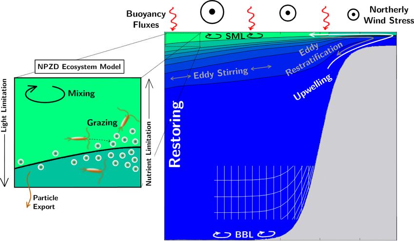
766                                                                                            J. E. Moscoso et al.: MAMEBUSv1.0

With these simplifications, the full equation for the physical        equations:
evolution of tracers is given by
                                                                        ∂ ū        ∂ φ̄     ∂         ∂ ū
                                                                             = fv−        +       κdia        ,                (11a)
                                                                        ∂t          ∂x ∂z              ∂z

                                                                        ∂ v̄             1     Ly     ∂          ∂ v̄
∂c                                 v  L                                      = −f u −      [φ]0 +           κdia        ,      (11b)
           = −∇ · (uc)           − [c]0 y                               ∂t             Ly            ∂z          ∂z
∂t    phys
             | {z }               Ly
            mean advection       | {z }                               ∇ · ū = 0,                                              (11c)
                              meridional advection
                                                                       ∂ φ̄
         −∇ · u? c −∇ · κiso ∇k c + ∂z (κdia ∂z c).                         = u,                                               (11d)

                                                                (9)    ∂z
         | {z } |       {z       } | {z }
         eddy advection      eddy stirring           mixing               b = gαθ .                                            (11e)

                                                                      Here, we have made the frictional–geostrophic approxima-
                                                                      tion (e.g., Edwards et al., 1998), assuming that the Rossby
The terms on the right-hand side of Eq. (9) are discussed fur-        number of the flow is small (e.g., Vallis, 2017), and thus that
ther in the following sections: in Sect. 2.2, we discuss the          momentum advection (second terms from the left in Eq. 10a–
evolution of the mean velocity u via the momentum equa-               10b) is negligible compared to other terms in the momentum
tions, and in Sect. 2.3 we discuss the subgrid-scale parame-          equation. This assumption may indeed have some limitations
terizations, i.e., eddy advection, eddy stirring, and mixing.         in upwelling regions with steep topography and strong strat-
                                                                      ification. Lentz and Chapman (2004) show that in the cross-
                                                                      shelf momentum flux divergence balances the wind stress
2.2    Momentum evolution equations                                   and supports an on shore return flow, which can impact ni-
                                                                      trate concentrations on the shelf (Jacox and Edwards, 2011).
                                                                         On the other hand, we have retained the time-evolution
To evolve a meridionally averaged tracer c using Eq. (9), the         terms (leftmost terms in Eq. 10a–10b) to allow forward evo-
meridionally averaged velocity field u3 is required. This ve-         lution of the horizontal velocity fields; if these terms were
locity field is evolved in MAMEBUS by solving a simplified            neglected, then these terms would need to be computed diag-
form of the hydrostatic Boussinesq momentum and continu-              nostically at each time step. The resulting system is almost
ity equations with a linear equation of state (Vallis, 2017):         identical to the T3W equations (Dauhajre and McWilliams,
                                                                      2018), a time-varying extension of the turbulent thermal
                                                                      wind balance (Gula et al., 2014), which was developed to ex-
                                                                    plain the circulation of submesoscale fronts. The meridional
    ∂u                       ∂φ   ∂       ∂u                          pressure gradient in Eq. (11a) is imposed, rather than solved
        = −u3 · ∇3 u + f v −    +    κdia      ,              (10a)
    ∂t                       ∂x ∂z        ∂z                          for prognostically, and is assumed to be set by the larger-
    ∂v                       ∂φ   ∂

                                          ∂v
                                                                     scale subtropical gyre circulation encompassing the EBUS,
        = −u3 · ∇3 v − f u −    +    κdia      ,              (10b)   which explicitly differs from the work done in Dauhajre
     ∂t                      ∂y ∂z        ∂z
                                                                      and McWilliams (2018) which focuses on more rapid time-
    ∂φ
        = b,                                                  (10c)   varying evolution on smaller scales. Together with the tracer
    ∂z                                                                advection equation for potential temperature (i.e., Eq. 9 with
∇3 · u3 = 0,                                                  (10d)   c = θ ), Eq. (11a)–(11e) comprise a closed set of equations
       b = gαθ.                                               (10e)   for the physical evolution of MAMEBUS.
                                                                         In Eq. (11c), we have invoked the earlier assumption that
                                                                      ∂v/∂y ≈ 0 (see Sect. 2.1), such that the averaged velocity
                                                                      field is non-divergent in the x–z plane. This implies that the
Here, φ = p/ρ0 is the dynamic pressure, where ρ0 is an ar-            zonal–vertical velocity field can be related to a mean stream
bitrary reference density, b is the buoyancy, θ is the potential      function ψ via
temperature, α is the thermal expansion coefficient (assumed
constant), g is the gravitational constant, and f is the Cori-               ∂ψ      ∂ψ
                                                                      u=−       , w=    .                                       (12)
olis parameter. Note that we have assumed that momentum                      ∂z      ∂x
is mixed by microscale turbulence following the same dif-
                                                                      These relationships allow us to calculate ψ and thus w, from
fusivity κdia as tracers (see Sect. 2.1), i.e., that the turbulent
                                                                      u, subject to the boundary conditions
Prandtl number (e.g., Kays, 1994) is exactly equal to 1.
   As in Sect. 2.1, we now meridionally average Eq. (10a)–            ψ = 0 at z = 0, z = ηb (x).                               (13)
(10e) to obtain evolution equations for u and v, and thus im-
plicitly also for w. This yields the following set of averaged        Here, z = ηb (x) is the mean sea floor elevation.

Geosci. Model Dev., 14, 763–794, 2021                                                     https://doi.org/10.5194/gmd-14-763-2021
J. E. Moscoso et al.: MAMEBUSv1.0 767
Additional boundary conditions are required to solve following Large et al. (1994) and Troen and Mahrt (1986).
Eq. (11a)–(11e) prognostically. Specifically, we require that The scaling factor of 27/4 ensures that GKPP (σsml ) has a
the vertical turbulent stress in Eq. (11a)–(11b) matches the maximum of 1 for 0 < σsml < 1.
wind stress applied at the sea surface and the drag stress at The diapycnal diffusivity in the bottom boundary layer,
the sea floor, with the latter formulated via a linear drag law. κbbl , is prescribed in the same way as κsml but over the depth
Formally, these boundary conditions are range ηb < z < ηb +Hbbl (x). Thus, analogous to Eq. (16), we
prescribe
∂u ∂v τy
κdia = 0, κdia = at z = 0, (14a) 0
∂z ∂z ρ0 κbbl (x, z) = κbbl GKPP (σbbl ), (18)
∂u ∂v
κdia = ru, κdia = rv at z = ηb (x). (14b) where the dimensionless bottom boundary layer vertical co-
∂z ∂z
ordinate is defined as σbbl = (z − ηb )/Hbbl .
Here, r is a linear drag coefficient and τ̄ y is the meridional At any point in space and time at which the water col-
wind stress. umn is statically unstable, i.e., when N 2 < 0, we increase the
value of κdia is increased locally to parameterize the effect
2.3 Physical parameterizations of density-driven convection. That is, we prescribe κconv fol-
lowing
In this section, we describe the parameterization of unre-
solved microscale mixing in the tracer evolution (Eq. 9) and ( 0
κconv , N 2 < 0,
the horizontal momentum (Eq. 11a–11b), and of mesoscale κconv = (19)
eddy advection and stirring in Eq. (9). This amounts to pa- 0, N 2 ≥ 0.
rameterizing the diapycnal diffusivity κdia , the isopycnal dif-
fusivity κiso , and the eddy velocity u? . Finally, the background diapycnal mixing, κbg (x, z), is sim-
ply prescribed as a constant background diffusivity. There are
2.3.1 Diapycnal mixing others that can be used (e.g., St. Laurent et al., 2002), but we
opt for simplicity in the first version of this model.
We formulate the diapycnal mixing coefficient κdia as a sum
of four distinct contributing processes: surface mixed layer 2.3.2 Eddy advection and isopycnal mixing
turbulence (κsml ), bottom boundary layer turbulence (κbbl ),
turbulence due to convective overturns within the water col- We now discuss the formulation of the eddy advection
umn (κconv ), and background mixing due to internal wave and isopycnal mixing terms in Eq. (9). As discussed in
breaking (κbg ). Formally, we write Sect. 2.1, we follow the assumptions and formalism of the
Gent and McWilliams (1990) and Redi (1982) parameteriza-
κdia (x, z, t) = κsml (x, z) + κbbl (x, z) tions, which are commonly used in ocean models that do not
+ κconv (x, z, t) + κbg (x, z). (15) explicitly resolve mesoscale eddies (e.g., Gent, 2011). These
parameterizations assume that eddy-induced fluxes of buoy-
The terms on the right-hand side of Eq. (15) are discussed in ancy and tracer diffusion are directed along isopycnal slopes
turn in the following paragraphs. and so must be augmented in the ocean’s surface mixed layer
The diapycnal diffusivity in the surface mixed layer, κsml , (SML) and bottom boundary layer (BBL). Here, the isopy-
is prescribed to have the same structure as that used in the κ- cnal slopes become very steep and isopycnals intersect the
profile parameterization (KPP) of Large et al. (1994). How- sea surface and floor (Tréguier et al., 1997). MAMEBUS
ever, for simplicity, the mixed layer depth Hsml (x) and maxi- therefore uses a modified form of the Ferrari et al. (2008)
mum magnitude κsml (x) are prescribed functions, rather than boundary layer parameterization, in which eddy buoyancy
depending on the local surface forcing. The vertical profile of and tracer fluxes are rotated through the SML and BBL in or-
κdia in the surface mixed layer, i.e., −Hsml < z < 0, is given der to enforce vanishing eddy-induced mass and tracer fluxes
by through the boundaries. Here, we summarize salient proper-
ties of this scheme, and in Appendix C we highlight differ-
0
κsml (x, z) = κsml GKPP (σsml ), (16) ences between our scheme and that of Ferrari et al. (2008).
The eddy-induced velocity u? = (u? , w ? ), introduced in
where the dimensionless surface mixed layer vertical coordi-
Eq. (8), is non-divergent by construction (see Appendix A)
nate σsml = −z/Hsml is defined such that 0 ≤ σsml ≤ 1 within
and so we write it as
the mixed layer. The structure function GKPP (σsml ) is given
by ∂ψ ? ∂ψ ?
u? = − , w? = , (20)
∂z ∂x
27 σsml (1 − σsml )2 , 0 ≤ σsml ≤ 1,
GKPP (σ ) = 4 (17) where ψ ? is the “eddy stream function”. This advecting
stream function is assumed to be the same for all tracers,
0, σsml ≥ 1,
https://doi.org/10.5194/gmd-14-763-2021 Geosci. Model Dev., 14, 763–794, 2021768 J. E. Moscoso et al.: MAMEBUSv1.0
which is accurate in the limit of small-amplitude fluctuations Surface mixed layer
of the velocity and tracer fields (Plumb, 1979), and takes the
form We now discuss the formulation of Ssml , the effective isopy-
cnal slope in the surface mixed layer. Following Ferrari et al.
ψ ? = κgm Sgm . (21) (2008), we construct Ssml in a way that avoids singularities
due to the vanishingly small vertical buoyancy gradients, and
Here, κgm is the Gent–McWilliams diffusivity and the Sgm
thus near-infinite isopycnal slopes, that occur in the mixed
is the is the Gent–McWilliams slope. The latter is conven-
layer. This is achieved by using the vertical buoyancy gradi-
tionally set equal to the mean isopycnal slope (Gent and
ent at the base of the mixed layer to define the effective slope
McWilliams, 1990):
as
Sint = −∂x b/∂z b. (22)
∂x b
Ssml = −Gsml (σsml ) , (28)
However, we allow Sgm to diverge from Sint in the SML and ∂z b|z=−Hsml
BBL, in part to ensure that the no-flux surface and bottom
boundary conditions are satisfied (Ferrari et al., 2008): where σsml = −z/Hsml is a dimensionless vertical coordi-
nate for the SML, as in Sect. 2.3.1. The corresponding eddy
ψ ? = 0 at z = 0, z = ηb (x). (23) stream function (Eq. 21) is identical to that of Ferrari et al.
(2008):
Specifically, we prescribe
∂x b
Ssml , −Hsml (x) < z < 0,
ψ ? = −κgm Gsml (σsml ) , z ≥ −Hsml . (29)
∂z b|z=−Hsml
Sgm = Sint , ηb (x) + Hbbl (x) < z < −Hsml (x), (24)
S , η (x) < z < η (x) + H (x).
bbl b b bbl The structure function Gsml (z) is required to enforce con-
tinuity of the vertical tracer fluxes and flux divergences at
The formulations of the modified slopes Ssml and Sbbl are the surface and at the base of the mixed layer. For example,
discussed below in the following sections (“surface mixed Eq. (23) requires that Gsml vanishes at the surface:
layer” and “bottom boundary layer” subsections).
The isopycnal mixing operator serves to mix tracers down Gsml (0) = 0. (30)
their mean gradients, in a direction that is parallel to mean
isopycnal surfaces in the ocean interior, following (Redi, We further require that the eddy stream function and eddy
1982). This may be written componentwise as residual tracer fluxes be continuous at the base of the SML,
i.e., that Ssml = Sint , which requires that
∂ ∂c ∂c
∇ · κiso ∇k c = κiso + κiso Siso Gsml (1) = 1. (31)
∂x ∂x ∂z
∂ ∂c 2 ∂c Finally, we require continuity of the divergence of the eddy
+ κiso Siso + κiso Siso , (25)
∂z ∂x ∂z tracer flux in order to avoid producing singularities at the
where Siso denotes the slope of the surface along which the SML base. The zonal and vertical components of the eddy
tracer is to be mixed and is assumed to be small (Siso
1). tracer flux are
Similar to Sgm , this slope is conventionally set equal to the
0 0
∂c ∂c ∂c
mean isopycnal slope Sint , but we apply modifications to the u c = κgm Sgm − κiso + Siso , (32a)
∂z ∂x ∂z
formulation of Siso in the SML and BBL to ensure that there
is zero eddy-induced tracer flux through the domain bound- ∂c ∂c ∂c
w 0 c0 = −κgm Sgm − κiso Siso + Siso . (32b)
aries, i.e., ∂x ∂x ∂z
κiso ∇k c · n̂ = 0 at z = 0, z = ηb (x), (26) It may be shown that continuity of ∇ · u0 c0 across z = −Hsml
is guaranteed if
where n̂ is a unit vector oriented perpendicular to the sea
surface or sea floor. Specifically, we prescribe ∂Ssml ∂Sint Hsml
= ⇒ G0sml (1) = , (33)
∂z +
z=−Hsml ∂z −
z=−Hsml λsml
Ssml , −Hsml (x) < z < 0,
Siso = Sint , ηb (x) + Hbbl (x) < z < −Hsml , (27) where λsml = ∂zz b/∂z b|z=−Hsml is a vertical length scale for
eSbbl , ηb (x) < z < ηb (x) + Hbbl (x). eddy motions at the base of the mixed layer.
The simplest form for Gsml (z) that satisfies conditions for
Thus, Sgm and Siso are identical everywhere above the BBL.
Eqs. (30), (31), and (33) is a quadratic function of depth:
The need for a distinction within the BBL is explained below
in the “surface mixed layer” and “bottom boundary layer” Hsml 2 Hsml
subsections. Gsml (σsml ) = − 1 − σsml + 2− σsml . (34)
λsml λsml
Geosci. Model Dev., 14, 763–794, 2021 https://doi.org/10.5194/gmd-14-763-2021J. E. Moscoso et al.: MAMEBUSv1.0 769
Equation (34) is currently implemented in MAMEBUS. A be aligned with the bottom slope at the sea floor, Sb = ∂x ηb
more sophisticated form of Gsml that arguably has stronger at z = ηb . We must therefore employ a modified effective
physical motivation is given by Ferrari et al. (2008). They slope e
Sbbl in the isopycnal mixing operator, as expressed in
split the SML into a true mixed layer, in which Gsml varies Eq. (27). We define eSbbl as
linearly (and so the eddy velocity is approximately uni-
form), overlying a transition layer, in which Gsml (σsml ) Sbbl = Sbbl + 1 − G
e ebbl (z) Sb , (41)
varies quadratically.
where Gebbl (σbbl ) is a modified structure function that also
Bottom boundary layer vanishes at the ocean bed:
ebbl (0) = 0.
G (42)
The scheme described above for the SML relies on the fact
that the ocean surface is approximately flat, which allows the Continuity of the eddy tracer fluxes at the top of the BBL
same effective slopes Ssml to be used for Sgm and Siso . The requires that
sloping sea floor requires separate BBL slopes, Sbbl and e Sbbl ,
and structure functions, Gbbl and Gebbl , to satisfy the required ebbl (1) = 1.
G (43)
conditions of no volume nor tracer flux through the boundary,
i.e., Eqs. (23) and (26). Finally, continuity of the eddy flux divergence is enforced by
Analogous to the SML, we define the effective slope Sbbl
as ∂G
ebbl
= 0. (44)
∂z
∂x b z=ηb +Hbbl
Sbbl = −Gbbl (σbbl ) , (35)
∂z b|z=ηb +Hbbl To satisfy Eqs. (42)–(44), we select a quadratic form for the
structure function G
ebbl (σbbl ):
where σbbl = (z−ηb (x))/Hbbl (x) is the BBL vertical coordi-
nate, as in Sect. 2.3.1. The eddy stream function in the BBL G
ebbl (σbbl ) = σbbl (2 − σbbl ). (45)
is therefore
2.4 Biogeochemical model formulation
? ∂x b
ψ = −κgm Gbbl (σbbl ) , z ≤ ηb + Hbbl . (36)
∂z b|z=ηb +Hbbl The current biogeochemical model implemented in MAME-
BUS is an NPZD (nutrient–phytoplankton–zooplankton–
To satisfy the condition of zero volume flux through the sea detritus) model. This NPZD model is modeled after the
floor, Eq. (23), the effective slope must vanish at z = ηb (x), size-structured AstroCAT (Banas, 2011) and Darwin models
which requires (Ward et al., 2012). For the purpose of this paper, we reduced
the size-structured ecosystem model to single phytoplankton
Gbbl (0) = 0. (37)
and zooplankton size classes, while preserving the option to
To ensure continuity of the eddy stream function at the top of run multiple size classes in future versions of the model. We
the BBL, we require that Sbbl approach Sint , i.e., also include a detritus variable, which allows for sinking and
export of organic matter away from the euphotic zone and
Gbbl (1) = 1. (38) redistribution of nutrients in the water column.
The biogeochemical equations in MAMEBUS are formu-
Finally, to ensure continuity of the eddy bolus velocity, we lated similarly to previous NPZD models but cast in terms
require that the gradient of Sgm be continuous at z = ηb + of the meridionally averaged nutrient, phytoplankton, zoo-
Hbbl . This imposes a constraint analogous to Eq. (33) on plankton, and detritus concentrations. We neglect additional
Gbbl : terms that would be introduced by first formulating the equa-
tions and then taking the meridional average, e.g., covari-
Hbbl
G0bbl (1) = − , (39) ances of the type P 0 Z 0 . This assumption is partially pred-
λbbl icated on the idea that zonal gradients in biogeochemical
where λbbl = bzz /bz z=η +H is a vertical length scale for tracers (e.g., nutrients and chlorophyll) are much stronger
b bbl than meridional gradients, as supported by observations and
eddies at the top of the BBL. To satisfy Eqs. (37)–(39), we
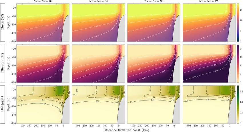
models (Fiechter et al., 2018). For example, Venegas et al.
select a quadratic form for the structure function Gbbl (σbbl ):
(2008) show that average chlorophyll concentrations during
Hbbl
Hbbl
the upwelling season vary approximately 2-fold in the north-
2
Gbbl (σbbl ) = − 1 + σbbl + 2 + σbbl . (40) ern California Current System, whereas observations from
λbbl λbbl
the California Cooperative Oceanic Fisheries Investigations
However, the effective slope Sbbl can no longer be used to de- (CalCOFI) (Fig. 7) show variations by an order of magni-
fine Siso in the BBL: Eq. (26) requires that the effective slope tude between nearshore and offshore stations. Along-shore
https://doi.org/10.5194/gmd-14-763-2021 Geosci. Model Dev., 14, 763–794, 2021770 J. E. Moscoso et al.: MAMEBUSv1.0
gradients in chlorophyll are observed along the coast, where where ϕ(I ) and ϕ(T ) are light- and temperature-limiting
they are driven by wind and topographic variations; however, functions, respectively. The light attenuation is modeled by
they are generally much smaller than the gradient between integrating the Beer–Lambert law, following Moore et al.
the coast and the offshore region (Fiechter et al., 2018). We (2001):
recognize that this is a simplification of the true variability
∂I (z)
in EBUSs, but we consider it appropriate on average over = −kpar I (z), where I0 = I (z = 0) = Qsw Ip , (48a)
the entire upwelling system, in particular within the ideal- ∂z
ized MAMEBUS framework, and plan to reassess it in future kpar = kw + P · kc , (48b)
work.
and the light-dependent uptake function is modeled follow-
We drop the bar notation indicating a meridional aver-
ing Sarmiento and Gruber (2006),
age for this section, with the understanding that all vari-
ables denote meridionally averaged quantities. In the follow- I (z)
ing, we include size-dependent uptake and grazing, along ϕ(I ) = q . (49)
I02 + I (z)2
with variable sinking speeds for detritus, to retain essen-
tial size-dependent biogeochemical interactions and export The temperature component of the uptake function is
fluxes. This will facilitate a future introduction of multiple
size classes in the model. All variables and coefficients are ϕ (T ) = e−rT (T −T0 ) . (50)
given in Table 1. We note that all of the parameter values and
equations described below measure time in days, whereas The maximum uptake rate is an allometric relationship de-
more generally MAMEBUS measures time in seconds; ap- fined as
propriate conversions are made in the model code to ensure bu
`p
dimensional consistency. The main conservation equations U max = au , (51)
`0
for biogeochemical tracers are
where `p is the user-determined phytoplankton size ex-
∂N pressed as equivalent spherical diameter (ESD), and `0 =
= −U(N, I, T , P ) + R(D), (46a)
∂t bio 1 µm is a normalized length scale, with all allometrically de-
∂P fined variables listed in Table 2. While there are other options
= U(N, I, T , P ) − G(P , Z) − M(P ), (46b)
∂t bio
for the bases of these allometric relationships outlined in this
∂Z section (e.g., cell volume), we make the decision to use ESD
= λG(P , Z) − M(Z), (46c) as a measure of cell size. Finally, the half-saturation coeffi-
∂t bio cient is kN = 0.1 mmol N m−3 .
∂D
= M(P ) + M(Z) + (1 − λ)G(P , Z)
∂t bio
2.4.2 Grazing
∂
− wsink D − R(D), (46d) Top-down processes are represented by zooplankton grazing
∂z on phytoplankton. Andersen et al. (2016) noted that there
where T (◦ C) is the model temperature, I (W m−2 ) is the is an optimal length scale for active predation and grazing,
local irradiance profile, N (mmol N m−3 ) is nitrate con- as a strategic trade-off for optimal biomass assimilation. We
centration, P (mmol N m−3 ) is phytoplankton concentra- make the assumption that the biomass assimilation of phy-
tion, Z (mmol N m−3 ) is zooplankton concentration, and D toplankton by zooplankton also follows Michaelis–Menten
(mmol N m−3 ) is the detritus concentration. The terms on the dynamics, then the functional form of grazing is given by
right-hand sides of Eq. (46a)–(46d) are explained in the fol- ϑP
lowing subsections. G(P , Z) = Gmax Z, (52)
kP + ϑP
2.4.1 Nutrient uptake where the maximum grazing rate is defined by an allometric
relationship defined as
Common controls on phytoplankton population are bottom-
bg
up limitation (i.e., nutrient control), and top-down grazing max `z
by zooplankton (Sarmiento and Gruber, 2006). We formu- G = ag , (53)
`0
late bottom-up controls using typical choices for light- and
temperature-dependent terms, and Michaelis–Menten uptake where d−1 represents a “per day” quantity. We define a Gaus-
(Sarmiento and Gruber, 2006). The functional form of uptake sian distribution about an optimal grazing length-scale fol-
is given by lowing Banas (2011):
N log (`p ) − log10 (`opt )
U(N, I, T , P ) = ϕ(I )ϕ(T )U max P, (47) ϑ = exp − 10 , (54)
N + kN 1`
Geosci. Model Dev., 14, 763–794, 2021 https://doi.org/10.5194/gmd-14-763-2021J. E. Moscoso et al.: MAMEBUSv1.0 771
Table 1. Parameters and values used in the ecosystem model implemented in MAMEBUS. Coefficients without explicit references are chosen
by the user.
Parameter Value Units Description Reference
Ip 0.45 Fraction of light available for photosynthesis (PAR) Moore et al. (2001)
kc 0.01 1 (mmol N)m−1 Absorption coefficient for photosynthesis Moore et al. (2001)
kp 3 mmol N m−3 Half-saturation coefficient for phytoplankton grazing Banas (2011)
kw 0.04 1 m−1 Absorption coefficient for water Moore et al. (2001)
1` 0.25 log10 µm Width of grazing profile Banas (2011)
`p 5 µm Length (ESD) of phytoplankton cell
`z 10 µm Length (ESD) of zooplankton cell
λ 0.33 Biomass assimilation efficiency
Qsw 340 W m−2 Surface irradiance Moore et al. (2001)
rT 0.05 1 ◦ C−1 Temperature dependence of nutrient uptake Ward et al. (2012)
rremin 0.04 1 d−1 Remineralization rate Ward et al. (2012)
T0 10 ◦C Reference temperature
µp 0.02 Phytoplankton mortality as a fraction of growth rate Banas (2011)
µz 0.97–12.57 m3 (mmol N d)−1 Density dependent zooplankton mortality Edwards and Bees (2001)
wsink 10 m d−1 Sinking speed of detritus
Table 2. Parameters and values used in the ecosystem model implemented in MAMEBUS. Coefficients without explicit references are chosen
by the user.
Parameter Value Units Description Reference
au 2.6 1 d−1 Uptake rate Tang (1995)
bu −0.45 Scaling parameter for uptake Tang (1995)
ag 26 1 d−1 Grazing rate Hansen et al. (1994)
bg −0.4 Scaling parameter for grazing Hansen et al. (1994)
ao 0.65 µm Optimal predator–prey length scale Hansen et al. (1994)
bo 0.56 Scaling parameter for optimal predator–prey interaction Hansen et al. (1994)
where 1` sets the width of the optimal grazing profile and toplankton mortality as
defines a band of grazing about the optimal prey size, `opt . By
allowing for a variable band of grazing, we are able to control M(P ) = µp U max P , (56)
the assimilation efficiency of phytoplankton by zooplankton
through direct preferential grazing. Accordingly, we model and zooplankton mortality as
the optimal prey size based on a preferential grazing profile
centered about an optimal predator–prey length scale: M(Z) = µz Z 2 . (57)
bo 2.4.4 Remineralization and particle sinking
`z
`opt = ao . (55)
`0 Sinking particles are an essential component of the verti-
cal transport of nutrients from the surface to the deep ocean
2.4.3 Mortality (Sarmiento and Gruber, 2006). Once particles sink past the
euphotic zone, they are remineralized and returned to the
Mortality closure terms often set important internal dynam- subsurface nutrient pool. In this model, we represent rem-
ics in ecosystem models (Poulin and Franks, 2010). While ineralization processes via a linear rate, i.e.,
linear mortality terms are generally used for phytoplank-
ton, zooplankton mortality is often modeled via a quadratic R(D) = rremin D, (58)
term to avoid unrealistic oscillations and stabilize the solu-
tion (Poulin and Franks, 2010). The quadratic mortality term where rremin is the specific remineralization rate.
may be rationalized as a representation of mixotrophic graz- Particles sink at a constant average speed in the water col-
ing, zooplankton self-grazing, and higher-order grazing in umn, following Eq. (46d). At the bottom boundary, we im-
NPZD models (Raick et al., 2006). Therefore, we model phy- pose zero sinking flux, i.e., wsink = 0 at z = ηb (x). Thus, any
https://doi.org/10.5194/gmd-14-763-2021 Geosci. Model Dev., 14, 763–794, 2021772 J. E. Moscoso et al.: MAMEBUSv1.0
nutrients that sink to the sea floor as detritus must remineral- 3.1 Formulation in terrain-following coordinates
ize there. This allows for redistribution of nutrients by mix-
ing within the bottom boundary layer, diffusion into the inte- We solve the model equations presented in Sect. 2 in a co-
rior, and transport via upwelling onto the shelf. ordinate system that “stretches” in the vertical to follow
the shape of the sea floor. Such a coordinate system avoids
2.5 Non-conservative terms “steps” in the sea floor that arise, for example, when using
geopotential vertical coordinates and allows fine vertical res-
In this section, we describe the treatment of all non- olution of the bottom boundary layer (e.g., Song and Haid-
conservative terms in the tracer evolution equation. MAME- vogel, 1994; Shchepetkin and McWilliams, 2003). Formally,
BUS allows arbitrary restoring of all tracers, which may be we make a coordinate transformation (x, z) → (x, σ ), where
used, for example, to impose offshore boundary conditions σ is a dimensionless vertical coordinate and is defined such
or to impose restoring at the sea surface. Fixed fluxes of all that σ = 0 at z = 0 and σ = −1 at z = ηb (x). This transfor-
tracers may also be imposed through the surface. More pre- mation requires a relationship between z and σ via a trans-
cisely, we formulate the non-conservative tracer tendency as formation function
∂c ∂c ∂c
= + . (59) z = ζ (x, σ ). (63)
∂t nct ∂t restore ∂t flux
The restoring and surface flux components of this tendency For example, a “pure” σ coordinate corresponds to the choice
are discussed separately below.
ζ (x, σ ) = −σ hb (x), (64)
2.5.1 Restoring
where hb (x) = −ηb (x) is the meridionally averaged water
The restoring of a tracer is represented as an exponential de- column thickness. However, this is not necessarily the most
cay to a prescribed, spatially varying tracer field, cr (x, z), practical choice for numerical applications, in which it is use-
with timescale tr (x, z). The tracer restoring is then formu- ful to focus the vertical resolution over certain depth ranges
lated as (especially those close to the top and bottom boundaries of
the ocean). MAMEBUS currently implements the UCLA-
∂c c − cr ROMS (Shchepetkin and McWilliams, 2005) transformation
=− . (60)
∂t restore tr function:
2.5.2 Tracer fluxes
hc σ + hb (x)C(σ )
ζ (x, σ ) = hb (x) . (65)
hc + hb (x)
Surface fluxes are represented as a tendency in the tracer con-
centration in the surface grid boxes. For an arbitrary tracer c, Here, C(σ ) is the stretching function, defined as
we formulate the surface flux term as follows:
c
∂Fflux
c
∂c Fflux,0 , z = 0, exp θb C̃(σ ) − 1
= , Fflux = (61) , θb > 0,
∂t flux ∂z 0, z < 0. C(σ ) = 1 − exp(−θb ) (66)
c
C̃(σ ), θb ≤ 0,
Here, Fflux,0 is the downward flux of c (units of [c]m s−1 )
at the surface. For the case of buoyancy, the surface flux is where
imposed as a surface energy flux, Qs (W m−2 ), with
1 − cosh(θs σ )
b gαQs , θs > 0,
Fflux,0 = , (62) C̃(σ ) = cosh(θs ) − 1 (67)
ρ0 Cp −σ 2 , θs ≤ 0.
where Cp = 4000 J K−1 kg−1 is the specific heat capacity.
Here, C and C̃ are the bottom and surface components of the
stretching function, respectively. The parameters θs ∈ [0, 10]
3 MAMEBUSv1.0 algorithm and θb ∈ [0, 4] are surface and bottom stretching parameters;
larger values cause the near-surface and near-bottom portions
In this section, we discuss the numerical solution of the of the domain to occupy larger fraction of σ space. The pa-
model equations presented in Sect. 2. This entails a recast- rameter hc defines a surface layer thickness, in which the co-
ing of the equations in terrain-following, or “sigma”, coor- ordinate system is approximately aligned with geopotentials,
dinates (e.g., Song and Haidvogel, 1994; Shchepetkin and provided that hb
hc .
McWilliams, 2003), followed by the spatial discretization of We now write the physical tracer evolution (Eq. 9) in σ
the equations and algorithms for numerical time stepping. coordinates. For a given function f = f (x, z(x, σ )), we can
Geosci. Model Dev., 14, 763–794, 2021 https://doi.org/10.5194/gmd-14-763-2021J. E. Moscoso et al.: MAMEBUSv1.0 773
write derivatives with respect to x and σ as column, Siso is equal to the isopycnal slope Sint , given by
∂f ∂f ∂ζ ∂f ∂b ∂b ∂b
= + , (68a) − Sσ
∂x ∂x ∂x ∂z x ∂x ∂x ∂z
σ z z σ x
Sint = − =−
∂f ∂ζ ∂f ∂b ∂b
= . (68b) ∂z ∂z
∂σ x ∂σ ∂z x x x
∂b
Using these identities, we may write the divergence of an
arbitrary vector F , with components F (x) and F (z) in the x̂ ∂x
σ
=− + Sσ . (72)
and ẑ directions, respectively, as ∂b
ζσ−1
∂σ
∂ ∂ x
∇ ·F = F (x) + F (z)
∂x z ∂z x Thus, the quantity Sint − Sσ can actually be computed more
∂ directly than the true isopycnal slope, as
= ζσ−1 ζσ F (x)
∂x σ ∂b
∂ (z)
∂x
+ ζσ−1 F − ζx F (x) . (69) σ
∂σ x Sint − Sσ = − . (73)
∂b
ζσ−1
Equation (69), combined with the definition of the mean ∂σ
x
stream function (Eq. 12), allows us to write the mean ad-
Finally, the σ coordinate transformation of the vertical
vection term in Eq. (9) as
(quasi-diapycnal) mixing operator is
∂ ∂c ∂ ∂c
!
∂ψ ∂ψ κdia = ζσ−1 κdia ζσ−1 . (74)
∇ · (uc) = ∇ · −c ,c ∂z x ∂z x ∂σ x ∂σ x
∂z ∂x
x z
! To summarize, we write Eq. (9) in σ coordinates as
∂ ∂ψ
= ζσ−1 −c ∂c
∂x σ ∂σ = Gadv + Giso + Gdia + Glat , (75)
x ∂t
! phys
∂ ∂ψ
+ ζσ−1 c . (70) where the tendency terms are
∂σ x ∂x
σ
∂ψ †
∂
Gadv = −ζσ−1 ζσ −c ζσ−1
An analogous expression may be obtained for the eddy ∂x σ ∂σ x
advection term, ∇ · (u? c), in Eq. (9), using the definition ∂
∂ψ †
(Eq. 21) of the eddy stream function. Next, we apply Eq. (69) − ζσ−1 c , (76a)
∂σ x ∂x σ
to the isopycnal mixing operator, defined by Eq. (25), in
Eq. (9) to obtain ∂ ∂c
Giso = ζσ−1 ζσ κiso
∂x σ ∂x σ
∂ ∂c
= ζσ−1 −1 ∂c
∇ · κiso ∇k c ζσ κiso +(Siso − Sσ )ζσ ,
σ ∂x ∂x σ ∂σ x
∂c ∂
∂c
+(Siso − Sσ )ζσ−1 + ζσ−1 κiso (Siso − Sσ )
∂σ x ∂σ x ∂x σ
∂ ∂c
+ ζσ−1 κiso (Siso − Sσ ) +(Siso − Sσ )ζσ−1
∂c
, (76b)
∂σ x ∂x σ ∂σ x
∂c
+(Siso − Sσ )ζσ−1
, (71) ∂ ∂c
∂σ x Gdia = ζσ−1 κdia ζσ−1 (76c)
∂σ x ∂σ x
where Sσ = ζx is the slope of surfaces of constant σ in x– v L
Glat = − [c] y . (76d)
z space, i.e., the slope of the σ coordinate grid lines. Thus, Ly 0
the isopycnal mixing operator is essentially just modified by
Here, we define
subtracting Sσ from Siso to obtain the mixing slope relative
to the slope of the σ coordinate grid. Over most of the water ψ† = ψ + ψ? (77)
https://doi.org/10.5194/gmd-14-763-2021 Geosci. Model Dev., 14, 763–794, 2021774 J. E. Moscoso et al.: MAMEBUSv1.0
all cell centers, corners, and faces:
(1z )j,k = zj,k+1/2 − zj,k−1/2 , (78c)
(1z )j +1/2,k = zj +1/2,k+1/2 − zj +1/2,k−1/2 , (78d)
(1z )j,k+1/2 = zj,k+1 − zj,k , (78e)
(1z )j +1/2,k+1/2 = zj +1/2,k+1 − zj +1/2,k , (78f)
where zj +1/2,k+1/2 denotes the physical elevation of each
grid point. Note again that $ is the velocity normal to the
upper and lower faces of the grid cell and so differs slightly
from the true vertical velocity w.
To compute the advective tendency, Gadv , the Kurganov
and Tadmor (2000) scheme requires a linear interpolation of
c over each grid cell. The linear slopes in the x and ζ di-
Figure 2. Illustration of the numerical grid used to compute solu- rections around cj,k (t) are calculated via slope-limited finite
tions to the model equations. differences between cj,k (t) and its adjacent grid points:
as the total advective or “residual” stream function (Plumb
cj +1,k − cj,k cj +1,k − cj −1,k
and Ferrari, 2005b), and we have added factors of ζσ in (∂x c)j,k = minmod θ , ,
Eq. (76a) so that the fluxes can be directly identified with the 1x 21x
zonal velocity, u† = −ζσ−1 ∂ψ † /∂σ |x , and the dia-σ veloc-
cj,k − cj −1,k
ity, $ † = ∂ψ † /∂x|σ . Note also that every derivative with re- θ , (79)
1x
spect to σ is multiplied by ζσ−1 , and that their product ζσ−1 ∂σ
cj,k+1 − cj,k cj,k+1 − cj,k−1
is equivalent to a derivative with respect to z. This allows us (∂z c)j,k = minmod θ , ,
to simplify the numerical discretization by avoiding explicit (1z )j,k+1/2 zj,k+1 − zj,k−1
references to σ coordinates and computing these derivatives cj,k − cj,k−1
θ , (80)
via finite differencing in z coordinates. (1z )j,k−1/2
3.2 Spatial discretization of the tracer evolution
equation
with parameter 1 < σ < 2. The “minmod” function evaluates
We solve Eq. (9) using the slope-limited finite-volume to zero if its arguments have differing signs and otherwise
scheme of Kurganov and Tadmor (2000) for systems of con- evaluates to its argument with smallest modulus. The cell
servation laws. We divide the domain into a grid of Nx by center estimates of the derivatives are then used to construct
Nζ cells, with uniform side lengths 1x and 1ζ in x/ζ space, two different estimates of c at each cell face via
as shown in Fig. 2. We store the cell-averaged value of c at
the center of the (j, k)th grid cell, which we denote as cj,k (t).
The mean, eddy, and residual stream functions are most nat- (−) 1
cj +1/2,k = cj,k + 1x (∂x c)j,k , (81a)
urally defined at the cell corners, as this allows a straightfor- 2
ward calculation of the residual velocities at the cell edges: (+) 1
cj +1/2,k = cj +1,k − 1x (∂x c)j +1,k , (81b)
2
ψj†+1/2,k+1/2 − ψj†+1/2,k−1/2 (−)
u†j +1/2,k = − , (78a) cj,k+1/2 = cj,k + (zj,k+1/2 − zj,k )(∂z c)j,k , (81c)
(1z )j +1/2,k
(+)
cj,k+1/2 = cj,k − (zj,k+1 − zj,k+1/2 )(∂z c)j,k+1/2 . (81d)
†
ψj†+1/2,k+1/2 − ψj†−1/2,k+1/2
$j,k+1/2 = . (78b)
1x
Here, we use 1z as a shorthand for the spatially varying ver- Finally, advective fluxes are determined at the cell faces us-
tical grid spacing, defined as a centered difference between ing an estimate of the maximum propagation speed in the
adjacent grid points. The vertical grid spacing is defined for system, which in our case is simply the residual velocity, and
Geosci. Model Dev., 14, 763–794, 2021 https://doi.org/10.5194/gmd-14-763-2021J. E. Moscoso et al.: MAMEBUSv1.0 775
thus the fluxes reduce to an upwind approximation: (2000) for parabolic operators.
(x)
(u) 1 h
(+) (−)
Hj +1/2,k = (1z )j +1/2,k (κiso )j +1/2,k
Fj +1/2,k = (1z )j +1/2,k u†j +1/2,k cj +1/2,k + cj +1/2,k
2
cj +1,k − cj,k
(+) (−)
i · + (Siso − Sσ )j +1/2,k
−|u†j +1/2,k | cj +1/2,k − cj +1/2,k , 1x
(82a) (∂z c)j,k + (∂z c)j +1,k
· , (87a)
2
($ ) 1h †
(+) (−)
Fj,k+1/2 = $j,k+1/2 cj,k+1/2 + cj,k+1/2 (σ )
2 Hj,k+1/2 = (κiso )j,k+1/2 (Siso − Sσ )j,k+1/2
i
† (+) (−)
−|$j,k+1/2 | cj,k+1/2 − cj,k+1/2 . (82b) (∂x c)j,k + (∂x c)j,k+1
·
2
For this version of the model, the formulation of the
cj,k+1 − cj,k
Kurganov and Tadmor (2000) scheme considers only the +(Siso − Sσ )j,k+1/2 , (87b)
(1z)j,k+1/2
maximum propagation speed of the momentum, u, and ex-
cludes the internal gravity wave speed which is supported where (∂z c)j,k , (∂z c)j +1,k , (∂x c)j,k , and (∂x c)j,k+1 are com-
with the momentum calculation in Sect. 2.2. As a result, this puted via Eq. (81a)–(81d). In the interior, the isopycnal dif-
would alter the overall advective fluxes; however, we omit fusion slope Siso = Sint and is calculated on cell corners via
this in the current version of the model and note that the full Eq. (85) and interpolated to cell faces via
formulation can be implemented here, but we choose to leave 1
this calculation to be updated in a future version of the model. (Siso )j +1/2,k = (Siso )j +1/2,k+1/2
2
The advective tendency in (x, z) space is then computed via
+(Siso )j +1/2,k−1/2 , (88a)
straightforward finite differencing of these fluxes:
1
(u) (u) (Siso )j,k+1/2 = (Siso )j +1/2,k+1/2
Fj +1/2,k − Fj −1/2,k 2
(Gadv )j,k = −
+(Siso )j −1/2,k+1/2 . (88b)
1x (1z )j,k
($ ) ($ ) v The diffusive tendency is then computed via straightforward
Fj,k+1/2 − Fj,k−1/2 Fj,k
− − . (83) finite differencing of the H fluxes:
(1z )j,k Ly
(x) (x)
Hj +1/2,k − Hj −1/2,k
The advective discretization (83) requires the residual stream (Giso )j,k = −
1x (1z )j,k
function to be known on all grid cell corners, which allows
(σ ) (σ )
the numerical fluxes to be computed at the cell edges. The Hj,k+1/2 − Hj,k−1/2
mean stream function ψ is computed from the mean velocity − . (89)
(1z )j,k
field via Eq. (12):
The tracer tendency due to diapycnal mixing, Gdia , is com-
k
X puted implicitly. During each time step, all other physical
ψ j +1/2,k+1/2 = − uj +1/2,k (1z )j +1/2,k . (84) and biogeochemical tendencies are computed and used to ad-
m=0 vance cj,k forward one time step 1t , i.e.,
The eddy stream function (Eq. 21) depends on the “true” c?j,k = cnj,k + F[cn ]. (90)
slope (Eq. 72) of the local b contours, which we discretize
Here, n denotes the time step number, and c? denotes an es-
as
timate of c at t + 1t (see Sect. 3.3 for details of the time-
(∂x b|z )j +1/2,k+1/2 stepping schemes). The updated tracer concentration is then
(Sint )j +1/2,k+1/2 = − . (85) further modified via the addition of a “correction” due to di-
(∂z b|x )j +1/2,k+1/2 apycnal diffusion. At each longitude, or for each j , we solve
The calculation of the derivatives with respect to x and z is cn+1 ?
j,k − cj,k 1
described in Sect. 3.5. We then construct ψ ? on cell corners =
1t zj,k+1/2 − zj,k−1/2
as
cn+1 n+1
"
j,k+1 − cj,k
· (κdia )j,k+1/2
ψj?+1/2,k+1/2 = (κgm )j +1/2,k+1/2 (Sint )j +1/2,k+1/2 . (86) zj,k+1 − zj,k
cn+1 n+1 #
The tracer tendency due to isopycnal diffusion, Giso , is dis- j,k − cj,k−1
−(κdia )j,k−1/2 . (91)
cretized following the formulation of Kurganov and Tadmor zj,k − zj,k−1
https://doi.org/10.5194/gmd-14-763-2021 Geosci. Model Dev., 14, 763–794, 2021776 J. E. Moscoso et al.: MAMEBUSv1.0
Equation (91) defines a tridiagonal matrix system of alge- ABIII method, in this version of the model as the default op-
braic equations for the unknowns {cn+1
j,k |k = 1. . .Nz }, which tion for time integration.
is inverted using the Thomas algorithm.
Finally, the meridional advection is discretized via a ABIII: c(tn+1 ) = c(tn )
straightforward upwind advection scheme: 1 1t 2 (21tn+1 + 31tn )
+ f n−2 n+1
(c)
vj,k 6 1tn−1 (1tn + 1tn−1 )
u
(Glat )j,k = cj,k − cj,k , 2 (21t
Ly 1tn+1 n+1 + 31tn + 31tn−1 )
−f n−1
(c) 1 † 1tn−1 1tn
vj,k = vj +1/2,k + vj†−1/2,k , (92) 2 +61t
1tn+1 (21tn+1
2 n+1 1tn +31tn+1
1tn−1 +61tn2 +61tn 1tn−1 )
+ fn
where v (c) denotes the meridional velocity on tracer points (1tn + 1tn−1 )1tn
and cu denotes the upstream tracer concentration, defined as
( N (95)
u
cj,k , v < 0,
cj.k = S , v > 0. (93) The first two time steps require the lower-order methods.
cj,k
We implement a forward Euler for the first time step and a
second-order AB scheme (defined below) for the second time
Here, cN and cS are the tracer concentrations at the northern
step:
and southern ends of the domain, respectively. In all of the
steps listed above, conditions of zero residual stream func- 1tn+1
ABII: c(tn+1 ) = c(tn ) + (2f (tn , c(tn ))1tn
tion and zero normal tracer flux are applied at the domain 21tn
boundaries. These conditions are imposed by simply setting + f (tn , c(tn ))1tn+1
ψ † to zero on all boundary points and by setting the numeri-
cal fluxes (F , H , etc.) to zero on the boundary cell faces. −f (tn−1 , c(tn−1 ))1tn+1 ) . (96)
Here, the notation 1tn indicates the nth time step. Deriva-
3.3 Temporal discretization
tions for the adaptive-time-stepping ABII and ABIII methods
MAMEBUS evolves the model equations forward in time are given in Appendix B.
using Adams–Bashforth (AB) methods Durran (e.g., 1991) 3.3.2 CFL conditions
modified to allow for adaptive-time-step sizes. In this section,
we outline the derivation of these methods and formally show MAMEBUS selects each model time step adaptively to en-
the derivation in Appendix B. We implement the adaptive- sure that time stepping is numerically stable. The time step is
time-step AB methods because this family of methods is nu- chosen to ensure that the CFL conditions for each of MAME-
merically stable with our scheme for the momentum equa- BUS’s various advective and diffusive operators, described in
tions (see Sect. 2.2). We then describe the constraints on the preceding subsections, are satisfied.
time step imposed by the Courant–Friedrichs–Lewy (CFL) The time step for advection of tracers is limited by the
condition. timescale associated with advective propagation across the
width of a grid box (1x or 1z ). These constraints can ap-
3.3.1 Adaptive-time-step Adams–Bashforth methods proximately be expressed as
Our time-integration scheme uses a family of time-step- 1x
variable Adams–Bashforth integrative methods. This specific 1t < , (97a)
|u| + uigw
formulation of the AB methods allows for the model time
1z
step to be adjusted dynamically following the CFL condi- 1t < (97b)
tions described in Sect. 3.3.2. Consider a tracer quantity c |w|
that evolves according to (Durran, 2010). Here, uigw is the maximum horizontal propa-
gation speed of internal gravity waves (Chelton et al., 1998):
∂c
= f (t, c(t)). (94) 1
Z
∂t cigw = N dz. (98)
π
Here, the function f conceptually represents the entire
model state, including the physical, biogeochemical, and Particulate sinking in the NPZD model is also calculated ex-
non-conservative tendencies. We make a note here that the plicitly and constrains the time step via a similar CFL crite-
diffusive component of the time-integration step is calculated rion:
implicitly and not included in the ABIII integration step (see (1z )
Eq. 91). We implement the third-order Adams–Bashforth, or 1t < , (99)
|wsink |
Geosci. Model Dev., 14, 763–794, 2021 https://doi.org/10.5194/gmd-14-763-2021You can also read