Simultaneous detection of ozone and nitrogen dioxide by oxygen anion chemical ionization mass spectrometry: a fast-time-response sensor suitable ...
←
→
Page content transcription
If your browser does not render page correctly, please read the page content below
Atmos. Meas. Tech., 13, 1887–1907, 2020
https://doi.org/10.5194/amt-13-1887-2020
© Author(s) 2020. This work is distributed under
the Creative Commons Attribution 4.0 License.

Simultaneous detection of ozone and nitrogen dioxide by oxygen
anion chemical ionization mass spectrometry: a fast-time-response
sensor suitable for eddy covariance measurements
Gordon A. Novak, Michael P. Vermeuel, and Timothy H. Bertram
Department of Chemistry, University of Wisconsin–Madison, Madison, WI, USA

Correspondence: Timothy H. Bertram (timothy.bertram@wisc.edu)

Received: 19 November 2019 – Discussion started: 25 November 2019
Revised: 20 February 2020 – Accepted: 21 February 2020 – Published: 15 April 2020

Abstract. We report on the development, characterization,         exchange from both stationary and mobile sampling plat-
and field deployment of a fast-time-response sensor for mea-      forms.
suring ozone (O3 ) and nitrogen dioxide (NO2 ) concentrations
utilizing chemical ionization time-of-flight mass spectrome-
try (CI-ToFMS) with oxygen anion (O−     2 ) reagent ion chem-    1   Introduction
istry. We demonstrate that the oxygen anion chemical ioniza-
tion mass spectrometer (Ox-CIMS) is highly sensitive to both      The deposition of O3 to the ocean surface is a significant
O3 (180 counts s−1 pptv−1 ) and NO2 (97 counts s−1 pptv−1 ),      component of the tropospheric ozone budget. Global chemi-
corresponding to detection limits (3σ , 1 s averages) of 13 and   cal transport model studies that explicitly treat O3 deposition
9.9 pptv, respectively. In both cases, the detection threshold    indicate that approximately one-third of total ozone dry de-
is limited by the magnitude and variability in the background     position is to water surfaces (Ganzeveld et al., 2009). How-
determination. The short-term precision (1 s averages) is bet-    ever, the magnitude of total annual global ozone deposition
ter than 0.3 % at 10 ppbv O3 and 4 % at 10 pptv NO2 . We          to ocean surfaces is highly sensitive to the deposition velocity
demonstrate that the sensitivity of the O3 measurement to         parameterization used, with model estimates ranging from 95
fluctuations in ambient water vapor and carbon dioxide is         to 360 Tg yr−1 (Ganzeveld et al., 2009; Luhar et al., 2017).
negligible for typical conditions encountered in the tropo-       Several common global chemical transport models including
sphere. The application of the Ox-CIMS to the measurement         GEOS-Chem (Bey et al., 2001), MOZART-4 (Emmons et al.,
of O3 vertical fluxes over the coastal ocean, via eddy covari-    2010), and CAM-chem (Lamarque et al., 2012) apply a glob-
ance (EC), was tested during the summer of 2018 at Scripps        ally uniform deposition velocity (vd ) that ranges between
Pier, La Jolla, CA. The observed mean ozone deposition ve-        0.01 and 0.05 cm s−1 depending on the model. In comparison
locity (vd (O3 )) was 0.013 cm s−1 with a campaign ensemble       to terrestrial measurements, where O3 dry deposition veloci-
limit of detection (LOD) of 0.0027 cm s−1 at the 95 % con-        ties are relatively fast (> 0.1 cm s−1 , Zhang et al., 2003), there
fidence level, from each 27 min sampling period LOD. The          is a paucity of direct observations of ozone deposition to
campaign mean and 1 standard deviation range of O3 mix-           the ocean surface necessary to constrain atmospheric models.
ing ratios was 41.2 ± 10.1 ppbv. Several fast ozone titration     Previous studies of O3 deposition to water surfaces have been
events from local NO emissions were sampled where unit            made from coastal towers (Gallagher et al., 2001), aircraft
conversion of O3 to NO2 was observed, highlighting instru-        (Faloona et al., 2005; Kawa and Pearson, 1989; Lenschow et
ment utility as a total odd-oxygen (Ox = O3 + NO2 ) sensor.       al., 1981), underway research vessels (Helmig et al., 2012),
The demonstrated precision, sensitivity, and time resolution      and in the laboratory (McKay et al., 1992), with observed
of this instrument highlight its potential for direct measure-    vd (O3 ) ranging between 0.01 and 0.15 cm s−1 . There is only
ments of O3 ocean–atmosphere and biosphere–atmosphere             one reported study of O3 deposition to freshwater, which
                                                                  showed a vd (O3 ) of 0.01 cm s−1 (Wesely et al., 1981). Mea-

Published by Copernicus Publications on behalf of the European Geosciences Union.
1888                                               G. A. Novak et al.: Simultaneous detection of ozone and nitrogen dioxide

sured deposition rates to snow and ice vary widely, with most      sensitivity detection on the order of 2.8 counts s−1 pptv−1
observations of vd (O3 ) from 0 to 0.2 cm s−1 , while models       (Bariteau et al., 2010; Pearson, 1990). A practical disadvan-
suggest vd (O3 ) from 0 to 0.01 cm s−1 (Helmig et al., 2007).      tage to this technique is the necessity of a compressed cylin-
Reactions of O3 with iodide and dissolved organic com-             der of NO which is highly toxic. Wet chemiluminescence
pounds (DOCs) in the ocean are known to play a controlling         techniques are used less, as they exhibit generally lower sen-
role in setting vd (O3 ) and may explain some of the variability   sitivity than dry chemiluminescence sensors and can be lim-
in observations (Chang et al., 2004; Ganzeveld et al., 2009).      ited by issues in the liquid flow (Keronen et al., 2003).
However, these quantities have not typically been measured            Dry chemiluminescence sensors have the simplest oper-
during field studies of vd (O3 ). To date there is no consensus    ation and have seen the most regular use for EC studies
on whether measured ocean O3 deposition velocities show            (Güsten et al., 1992; Tuovinen et al., 2004). However, dry
a wind speed dependence (Fairall et al., 2007). The most           chemiluminescence sensor discs require conditioning with
comprehensive dataset is from Helmig et al. (2012), which          high ozone (up to 400 ppbv for several hours) before opera-
reported a deposition velocity range of 0.009–0.034 cm s−1         tion, are known to degrade over time, and have high variabil-
from 1700 h of observation over five research cruises. This        ity in sensitivity between sensor discs (Weinheimer, 2007).
dataset showed variability in vd (O3 ) with wind speed (U10 )      These factors have led to limitations in long-term stabil-
and sea surface temperature (SST), highlighting the need for       ity and to uncertainty in calibration factors for dry chemi-
further field observations as constraints for model parameter-     luminescence sensors, resulting in uncertainty in the accu-
izations.                                                          racy of the flux measurement (Muller et al., 2010). Muller
   The small magnitude of O3 ocean–atmosphere vertical             et al. (2010) also reported a comparison of two identical
fluxes presents a significant analytical challenge for exist-      colocated dry chemiluminescence sensors with half-hourly
ing ozone sensors used in eddy covariance (EC) analyses.           flux values differing by up to a factor of 2 and a mean
Driven in part by stringent sensor requirements for EC tech-       hourly flux difference ranging from 0 % to 23 % between
niques, significant uncertainties in the magnitude of and vari-    sensors. Recently Zahn et al. (2012) reported the develop-
ability in ozone deposition to water surfaces remain. In con-      ment of a commercial dry chemiluminescence ozone detec-
trast, O3 vertical fluxes to terrestrial surfaces are 10 to 100    tor capable of fast (> 10 Hz) measurements with high sensi-
times faster than to water surfaces, significantly loosening       tivity (∼9 counts s−1 pptv−1 ) suitable for EC or mobile plat-
sensor precision requirements. Nonetheless, significant vari-      form sampling. However, they also report issues of short- and
ability in vd (O3 ) exists between surface types (e.g., soil vs.   long-term drift and variability between sensor discs. These
leaf; Wesely and Hicks, 2000). Terrestrial deposition veloci-      accuracy and drift concerns have driven an interest in the de-
ties also show strong diel and seasonal variability due to fac-    velopment of a new, stable, and fast ozone sensor suitable for
tors such as stomatal opening and within-canopy chemistry          EC measurements from both stationary and mobile sampling
(Fares et al., 2010; Fowler et al., 2001; Kurpius and Gold-        platforms.
stein, 2003). Highly accurate and precise measurements of             In addition to the inherently small magnitude of vd (O3 ),
O3 are required to correctly model the response of vd (O3 ) to     the fast chemical titration of O3 by NO (Reaction R1) often
each of these factors. While terrestrial and ocean exchange        complicates the interpretation of vd (O3 ) measurements. Sur-
studies have substantial differences in experimental design,       face emissions of NO result in a high bias in the measured
a sensor suitable for ocean–atmosphere ozone deposition            deposition velocity when the titration Reaction (R1) is fast
measurements via EC is expected to be highly capable of            relative to the transport time to the height of the sensor.
biosphere–atmosphere measurements due to the significantly
larger deposition rates and similar accuracy requirements.         O3 + NO → NO2 + O2            k(O3 + NO)
   Eddy covariance measurements typically require fast (1–                   = 1.8 × 10   −14
                                                                                                cm3 molecule−1 s−1          (R1)
10 Hz), high-precision sensors in order to resolve covariance
on the timescales of the fastest atmospheric turbulent eddies.     Surface NO emissions from both biogenic and anthro-
Due to this constraint, standard O3 monitoring instruments         pogenic sources are widespread, with ocean emissions on
which utilize UV-absorption detection do not have a suitable       the order of 1×10⁸ molecules cm−2 s−1 (Zafiriou and Mc-
time response or suitable precision for EC measurements,           Farland, 1981) and soil emissions ranging from 5 × 10⁹
and ozone flux measurements have primarily utilized fast-          to 2 × 10¹¹ molecules cm−2 s−1 (Yienger and Levy, 2004).
response chemiluminescence sensors. Chemiluminescence              These emissions correspond to a positive bias in the observed
detectors can use either gas-phase, dry, or wet reagents for       vd (O3 ) dry deposition rate on the order of 5 % in the marine
detection with important differences between them (Muller          atmosphere (discussed in Sect. 3.7.1) and up to 50 % in a
et al., 2010). Gas-phase chemiluminescence sensors are typ-        forested site (Dorsey et al., 2004). Simultaneous flux detec-
ically based on the reaction of O3 with nitric oxide (NO) to       tion of O3 with one or both of NO or NO2 is commonly used
form an excited state NO2 ∗ which then relaxes to the ground       to address this flux divergence problem (Finco et al., 2018;
state, emitting a photon that can be detected. This method         Stella et al., 2013). However, these studies typically require
has well-understood reaction kinetics and allows for high-         separate sensors for O3 and NOx which can introduce addi-

Atmos. Meas. Tech., 13, 1887–1907, 2020                                             www.atmos-meas-tech.net/13/1887/2020/
G. A. Novak et al.: Simultaneous detection of ozone and nitrogen dioxide                                                       1889

tional sources of uncertainty. Related challenges of fast O3      only quadrupole chamber held at 1.4×10⁻² mbar and a final
titration exist for quantification of O3 from mobile platforms    chamber containing focusing optics which prepare the ion
where there is dynamic sampling of different air masses with      beam for entry into the compact ToF mass analyzer (CToF,
potentially differing O3 –NO–NO2 steady-state conditions.         TOFWERK AG and Aerodyne Research Inc.). The mass re-
   In what follows, we describe the characterization and first    solving power (M/1M) of the instrument as configured for
field observations of a novel oxygen anion chemical ioniza-       these experiments was greater than 900 at −60 m/Q. All
tion time-of-flight mass spectrometer (Ox-CIMS) sensor for        ion count rates reported here are for unit mass resolution
O3 and NO2 . Over the past 2 decades, chemical ionization         integrated peak areas. In this work extraction frequencies
mass spectrometry (CIMS) techniques have emerged as sen-          of 75 kHz were used, resulting in mass spectra from 27 to
sitive, selective, and accurate detection methods for a diverse   327 −m/Q. All mass spectra were saved at 10 Hz for analy-
suite of reactive trace gases (Huey, 2007). Successful appli-     sis.
cation of CIMS for EC flux measurements have been demon-
strated from many sampling platforms including ground sites       2.2   Oxygen anion chemistry
(Kim et al., 2014; Nguyen et al., 2015), aircraft (Wolfe et
al., 2015), and underway research vessels (Blomquist et al.,      Oxygen anion (O−   2 ) reagent ion chemistry has been investi-
2010; Kim et al., 2017; Yang et al., 2013) employing a vari-      gated previously for its use in the detection of nitric acid and
ety of reagent ion chemistry systems. Here we demonstrate         more recently hydrogen peroxide (Huey, 1996; O’Sullivan et
the suitability of the Ox-CIMS for EC flux measurements           al., 2018; Vermeuel et al., 2019). Oxygen anion chemistry
and provide detailed laboratory characterization of the instru-   has also been used for chemical analysis of aerosol particles
ment.                                                             in a thermal-desorption instrument, primarily for detection of
                                                                  particle sulfate and nitrate (Voisin et al., 2003). Oxygen anion
                                                                  chemistry has also been used for the detection of SO2 via a
                                                                  multistep ionization process where CO−     3 reagent ions are first
2     Laboratory characterization
                                                                  generated by the reaction of O−  2 with   added  excess O3 in the
                                                                  presence of CO2 . The CO−    3 reagent  ion  then ligand switches
2.1    Chemical ionization time-of-flight mass
                                                                  with SO2 to form SO−   3  which  then quickly   reacts with ambi-
       spectrometer
                                                                  ent O2 to form the primary detected SO−       5 product (Porter et
A complete description of the CI-ToFMS instrument (Aero-          al., 2018; Thornton et al., 2002a). Ionization of analytes by
dyne Research Inc., TOFWERK AG) can be found in                   oxygen anion reagent ion chemistry proceeds through both
Bertram et al. (2011). In what follows we highlight signifi-      charge transfer (Reaction R2) and adduct formation (Reac-
cant differences in the operation of the instrument from what     tion R3).
is discussed in Bertram et al. (2011). Oxygen anions are gen-     O2 (H2 O)−                      −
                                                                           n + A → O2 (H2 O)n + A                              (R2)
erated by passing an 11 : 1 volumetric blend of ultrahigh-
                                                                  O2 (H2 O)−
                                                                           n +B     →B    · O2 (H2 O)−
                                                                                                     n                         (R3)
purity (UHP) N2 and O2 gas (both Airgas 5.0 grade) through
a polonium-210 α-particle source (NRD, P-2021 Ionizer).           It is expected that charge transfer from oxygen will occur to
This N2 : O2 volume ratio was found empirically to maxi-          any analyte with an electron affinity (EA) greater than O2
mize the total reagent ion signal in our instrument while min-    (0.45 eV; Ervin et al., 2003), resulting in a relatively non-
imizing background signal at the O3 detection product (CO−  3,    specific reagent ion chemistry (see Rienstra-Kiracofe et al.,
−60 m/Q). Further discussion of the reagent ion chemistry         2002, for a compilation of molecular EA values) Adduct for-
and precursor concentration can be found in Sect. 2.2 and 2.8.    mation is observed when the binding enthalpy of the adduct
The reagent ion stream then mixes with ambient air in an          is larger than that of the oxygen–water adduct and the adduct
ion–molecule reaction (IMR) chamber held at 95 mbar where         is stable enough to be preserved through the ion optics. This
product ions were generated. Further discussion of the de-        adduct formation framework is analogous to what has been
pendence of instrument sensitivity on IMR pressure can be         shown for iodide reagent ion chemistry (Lee et al., 2014).
found in Sect. 2.6. At this pressure, the residence time in          The O−  2 reagent ions present in the IMR are expected to
the IMR is estimated to be on the order of 100 ms. Prod-          have a series of attached water molecules at ambient hu-
uct ions then pass into three differentially pumped chambers      midity and the IMR pressure (95 mbar) and electric field
before reaching the ToF mass analyzer. Ions first move from       strengths used in this study (Bork et al., 2011). The reagent
the IMR to a collisional dissociation chamber (CDC) held at       ion is therefore reported as O2 (H2 O)−n for the remainder of
2 mbar which houses a short-segmented RF-only quadrupole          this work. In the recorded mass spectra from our instrument,
ion guide. Field strengths in the IMR and CDC were tuned to       all the reagent ion signal is observed as n = 0–1 (i.e., O− 2
be as soft as possible to preserve the transmission of weakly     and O2 (H2 O)− ) as seen in Fig. 1. Oxygen anion–water clus-
bound clusters while still maintaining acceptable total ion       ters larger than n = 1 are likely present in the IMR but H2 O
signals (ion optic potentials are listed in Table S1 in the       evaporates off the cluster in the CDC before detection due
Supplement). Ions then sequentially pass into a second RF-        to the lower binding enthalpy of each additional water in

www.atmos-meas-tech.net/13/1887/2020/                                                Atmos. Meas. Tech., 13, 1887–1907, 2020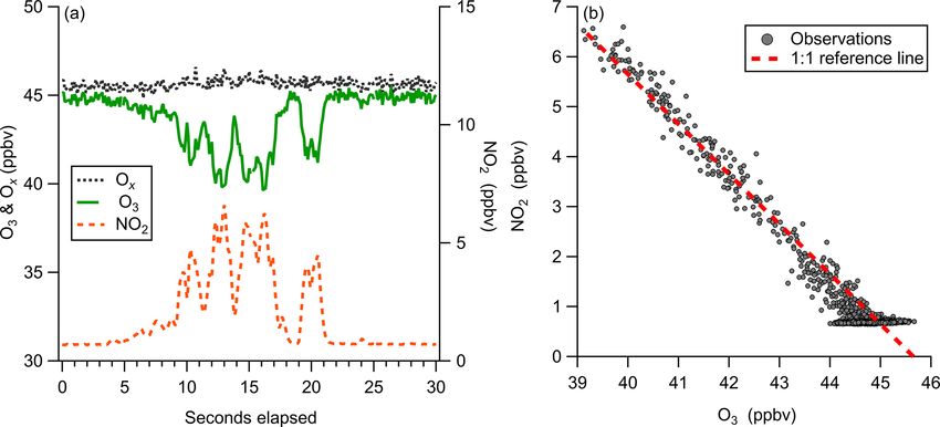
1890                                                 G. A. Novak et al.: Simultaneous detection of ozone and nitrogen dioxide

                                                                      the mass spectrometer, but it may exist in the IMR and disso-
                                                                      ciate as it transfers into the CDC prior to detection. A small
                                                                      amount of ozone is detected directly as O−    3 , but the mag-
                                                                      nitude of this signal is less than 1 % of the signal of CO−   3
                                                                      during ambient sampling. The proposed mechanism of CO−        3
                                                                      formation is supported by a study using isotopically labeled
                                                                      oxygen to form labeled ozone anions (18 O−  3 ) in a corona dis-
                                                                      charge source which then reacted with CO2 to form the de-
                                                                      tected product C18 OO−   2 (Ewing and Waltman, 2010). This
                                                                      product supports a single oxygen being transferred from the
                                                                      ozone anion to carbon dioxide (as in Reaction R5a).

                                                                                           −
                                                                      NO2 + O2 (H2 O)−
                                                                                     n → NO2 + O2 + nH2 O                        (R6)

                                                                      Oxygen anions are expected to be a highly general reagent
                                                                      ion chemistry, showing sensitivity to an array of analytes.
Figure 1. Ox-CIMS mass spectra collected at 1 Hz and mass reso-       While the focus of this work is on detection of O3 and NO2 ,
lution of 950M/1M (at −60 m/Q), with major peaks highlighted.         detection of hydrogen peroxide, nitric acid, formic acid, sul-
O−                   −
  2 and O2 (H2 O) at −32 m/Q and −50 m/Q, respectively,               fur dioxide, and other species with the Ox-CIMS has demon-
are the two observed forms of the reagent ion. The detected ozone     strated good performance (Vermeuel et al., 2019). An ex-
product (CO− 3 , −60 m/Q) is of comparable magnitude to the O2
                                                                  −
                                                                      ample ambient mass spectrum recorded at 1 Hz sampling is
reagent ion during ambient sampling. NO2 is detected as the charge
                                                                      shown in Fig. 1, with several major peaks highlighted. Also
transfer product NO− 2 at −46 m/Q. Masses greater than −150 m/Q
contribute less than 2 % to the total signal and are not plotted.
                                                                      apparent are an abundance of peaks throughout the spectra
                                                                      with high signal intensity. During ambient observations, over
                                                                      one-third of masses from −m/Q 27–327 showed a signal in-
O2 (H2 O)−                                                            tensity greater than 1 × 10⁴ counts per second (cps). A larger
          n (Bork et al., 2011) and the high field strength at
the exit of the CDC (Brophy and Farmer, 2016). Variability            survey and classification of oxygen anion reagent ion chem-
in the number of attached water molecules (n) as a function           istry to utilize this versatility is underway.
of humidity introduces the possibility of a water dependence
                                                                      2.3   Laboratory calibration
on the ion chemistry, which is discussed further in Sect. 2.5.
   The detection of ozone (O3 ) by oxygen anion reagent ion           Laboratory calibrations of the Ox-CIMS were performed to
chemistry proceeds via a two-step reaction leading to the for-        determine instrument sensitivity to O3 and NO2 . Ozone was
mation of a carbonate anion (CO−    3 ), which is the final de-       generated by passing UHP Zero Air (ZA, Airgas 5.0 grade)
tected product. First, the oxygen anion (O2 (H2 O )−   n ) either     through a mercury lamp UV source (Jelight Co, Irvine, CA).
transfers an electron to ozone-forming O− 3 (Reaction R4a) or         Outflow from the lamp source was diluted in UHP ZA and
forms a stable cluster with ozone (Reaction R4b). The ozone           split between the Ox-CIMS and a factory-calibrated 2B per-
anion (either bare or as a cluster with O2 (H2 O)n ) then reacts      sonal ozone monitor (POM; 2B Technologies) with an ac-
with a neutral CO2 molecule to form CO−     3 (Reaction R5a–          curacy of ±1.5 ppbv, which served as our reference stan-
5b) which is the primary detected product in the mass spec-           dard. Ozone concentrations were varied over the range 0–80
trometer. The electron affinity of O3 is 2.1 eV (Arnold et al.,       ppbv and instrument response was determined to generate a
1994).                                                                calibration curve. NO2 was delivered from a certified stan-
                   −                                                  dard cylinder (Scott-Marrin, 4.84 ± 0.1 ppmv). The primary
O3 + O2 (H2 O)−
              n → O3 + O2 + nH2 O                           (R4a)     NO2 standard was diluted in UHP ZA to span the range of
O3 + O2 (H2 O)−
              n    →   O2 (O3 )(H2 O)−
                                     n                      (R4b)     0–10 ppbv. Dilutions of calibration standards were made in
                                                                      UHP ZA which was humidified to the desired amount by
                                                                      splitting a portion of the flow through a bubbler containing
                                                                      18 M water. CO2 (Airgas Bone Dry grade) was added to
O−           −
 3 + CO2 → CO3 + O2                                         (R5a)     the dilution flow to maintain mixing ratios of 380 ppmv for
                          −
O2 (O3 )(H2 O)−
              n + CO2 → CO3 + 2O2 + nH2 O                   (R5b)     all calibrations (See Sect. 2.6). A Vaisala HMP110 sensor
                                                                      continuously measured relative humidity (RH) and tempera-
It is not clear whether it is the bare ozone anion (Reac-             ture inline downstream of the Ox-CIMS and POM inlets. All
tions R4a and R5a) or the cluster (Reactions R4b and R5b)             flows were controlled by mass flow controllers (MKS Instru-
that goes on to react with CO2 to form the carbonate an-              ments, 1179C series) with an estimated total uncertainty of
ion. The O2 (O3 )(H2 O)−
                       n product has not been observed in             10 %. Example calibration curves for O3 and NO2 are shown

Atmos. Meas. Tech., 13, 1887–1907, 2020                                                 www.atmos-meas-tech.net/13/1887/2020/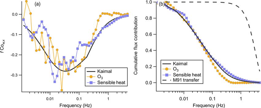
G. A. Novak et al.: Simultaneous detection of ozone and nitrogen dioxide                                                              1891

Table 1. Summary of instrument sensitivity, precision, and accuracy for detection of O3 and NO2 from laboratory calibrations. Sensitivity is
reported at a specific humidity (SH) of 8 g kg−1 which corresponds to 40 % RH at 25 ◦ C. All limits of detection (LODs) are for a signal-to-
noise ratio (S / N) of 3. The optimum LOD is reported as the LOD at the optimum averaging time determined by the minimum of the Allan
variance spectrum. Optimum averaging times were determined to be 11 s for O3 and 19 s for NO2 . The reported field comparison (R 2 ) is
from a regression of 1 min bin averaged ozone concentration from the Ox-CIMS with an EPA (Environmental Protection Agency) monitor
(Thermo Fisher 49i) in Zion, Illinois, during 4 weeks of ambient observation shown in Fig. 7.

   Species    Normalized                 Absolute           LOD        LOD         LOD        Background     Precision    Field
              sensitivity                sensitivity        optimum    (1 Hz)      (10 Hz)    (cps, 1σ )     (10 Hz)      calibration R 2
              (8 g kg−1 SH, 1σ )         (8 g kg−1 SH)
   O3         12.4 ± 1.2 ncps pptv−1     180 cps pptv−1     4.0 pptv   13 pptv     42 pptv    3.1 × 10⁵      0.74 %       0.99
                                                            (11 s)                            ±5.0 × 10⁴
   NO2        6.7 ± 1.0 ncps pptv−1      97 cps pptv−1      2.3 pptv   9.9 pptv    32 pptv    5.1 × 10⁴      1.1 %        –
                                                            (19 s)                            ±1 × 10⁴

                                                                        formation chemistry for a given analyte sets a fundamental
                                                                        limit on sensitivity for a given instrument configuration. Sen-
                                                                        sitivity values can be normalized by scaling all signals to a
                                                                        fixed total reagent ion signal of 1 × 10⁶ cps to isolate the sen-
                                                                        sitivity component controlled by reagent ion chemistry, sep-
                                                                        arate from changes in instrument performance due to decay
                                                                        in the ion source or other factors. The total reagent ion signal
                                                                        is taken as the sum of the O−                  −
                                                                                                       2 and O2 (H2 O) signals. Sensi-
                                                                        tivity values through the remainder of the text are reported as
                                                                        either absolute sensitivities in counts per second (cps pptv−1 )
Figure 2. Normalized calibration curves of O3 (a) and NO2 (b)           or normalized sensitivities in normalized counts per second
at 8 g kg−1 specific humidity (approximately 40 % RH at 25 ◦ C).        (ncps pptv−1 ). Absolute sensitivity values control instrument
Ozone is detected as CO−  3 at −60 m/Q. NO2 is detected as the          limits of detection (LODs) and precision, while normalized
charge transfer product (NO−2 ) at −46 m/Q. Error bars are the stan-
                                                                        sensitivities are used for comparison of calibration factors.
dard deviation in normalized count rate for each measurement point.
                                                                        2.5     Dependence of instrument sensitivity on specific
                                                                                humidity
in Fig. 2. An overview of instrument sensitivity, limits of de-
tection (LODs), and precision for O3 and NO2 is given in                The dependence of instrument sensitivity on ambient wa-
Table 1.                                                                ter content was assessed for specific humidity (SH) ranging
                                                                        between 0 and 16 g kg−1 (approximately 0 %–80 % RH at
2.4   Absolute sensitivity                                              25 ◦ C) by triplicate calibrations as shown in Fig. 3. Sensitiv-
                                                                        ity to O3 had no significant dependence on specific humidity
The absolute sensitivity of the Ox-CIMS for detection of                over the range 4–16 g kg−1 . Sensitivity to NO2 has a specific
analytes is controlled by the kinetics and thermodynamics               humidity dependence over the range 4–16 g kg−1 , decreas-
of the reagent ion chemistry and the total ion generation               ing from 7.9 to 4.6 ncps pptv−1 . A 30 % and 45 % decline
and transmission efficiency of the instrument. Under the op-            in sensitivity was observed from 0 to 4 g kg−1 for O3 and
erational configuration described in Sect. 2.1, the typical             NO2 , respectively. This low-humidity range is rarely sam-
reagent ion signal (O2 − + O2 (H2 O)− n ) ranged from 0.8 to            pled in the boundary layer over water surfaces but may be
2.2 × 10⁷ counts s−1 (Fig. S1 in the Supplement). The mean              significant in some terrestrial or airborne deployments and
total reagent ion signal over 6 weeks of ambient sampling               would require careful calibration. The SH range from 8 to
(Sect. 3.1) was 1.45 × 10⁷ cps. The absolute instrument sen-            16 g kg−1 corresponds to approximately 40 % to 80 % RH
sitivity at this reagent ion signal to O3 and NO2 is 180                at 25 ◦ C which is typical of the humidity range over mid-
and 97 cps pptv−1 , respectively, (at 8 g kg−1 SH). Total in-           latitude oceans (Liu et al., 1991). Ab initio calculations of
strument count rate is a complex function of instrument de-             O2 − (H2 O)n and O3 − (H2 O)n clusters performed by Bork et
sign, instrument ion optics tuning, Po-210 source decay, mi-            al. (2011) showed that charge transfer from the bare (n = 0)
crochannel plate (MCP) detector decay, and ToF extraction               O−                                               −1
                                                                          2 to O3 was exothermic at ca. −160 kJ mol . At larger
frequency, all of which either are tunable parameters or vary           cluster sizes of n = 4–12, charge transfer becomes less fa-
in time. Conversely, the reagent ion charge transfer or adduct          vorable and converges to ca. −110 kJ mol−1 . An increase in

www.atmos-meas-tech.net/13/1887/2020/                                                        Atmos. Meas. Tech., 13, 1887–1907, 2020
1892                                                   G. A. Novak et al.: Simultaneous detection of ozone and nitrogen dioxide

Figure 3. Dependence of O3 and NO2 sensitivities on specific hu-
midity. Error bars indicate standard deviation of triplicate calibra-   Figure 4. Ox-CIMS cumulative sensitivity to O3 detected either di-
tion curves. The shaded blue region of SH 8–16 g kg−1 is the ap-        rectly as O−          −
                                                                                   3 or as CO3 as a function of CO2 mixing ratio. The sum
proximate typical range of specific humidity in the midlatitude ma-     of sensitivity as O3 and CO−
                                                                                           −
                                                                                                     3 shows that total sensitivity to O3 is
rine boundary layer.                                                    conserved as the product distribution shifts with CO2 mixing ratio.
                                                                        More than 99 % of O3 is observed as CO−     3 at CO2 mixing ratios
                                                                        greater than 60 ppmv.
n from 0 to 4 over the SH range 0–4 g kg−1 is a potential ex-
planation for the initial decline in sensitivity observed with
SH before leveling off from 4 to 16 g kg−1 . It is not known            bient O3 mixing ratio of 100 ppbv. An exponential fit of the
if the enthalpy of charge transfer from O2 − (H2 O)n to NO2             O−                                     −
                                                                          3 product vs. CO2 indicates that O3 makes up less than
follows a similar trend with n. Ion mobility studies to deter-          1 % of the detected ozone at CO2 mixing ratios greater than
mine the O2 − (H2 O)n cluster size with SH and IMR pressure             10 ppmv. This suggests ambient samples will always have
would provide valuable insight into the observed dependence             a substantial excess of CO2 necessary to drive the reaction
of sensitivity on water content.                                        completely to the CO−  3 product. The measured flat response
                                                                        from 60 to 500 ppmv CO2 indicates that natural variability in
2.6    Dependence on CO2                                                ambient CO2 will have negligible impact on ambient mea-
                                                                        surements of ozone. No other analytes that we have cali-
The ionization pathway for detection of O3 with O2 − (H2 O)n            brated for with the Ox-CIMS (HCOOH, HNO3 , H2 O2 ) have
reagent ion chemistry differs from typical chemical ioniza-             shown a CO2 mixing ratio dependence, suggesting that CO2
tion schemes in that it involves a two-step reaction of charge          may be uniquely involved in the detection of O3 and is not a
transfer to ozone-forming O−   3 , which then reacts with CO2 to        general feature of the oxygen anion chemistry. All other re-
form the detected CO−   3  product   (Reactions R4–R5). There-          ported laboratory calibrations reported here were performed
fore, we assessed the impact of the CO2 mixing ratio in the             at CO2 mixing ratios of 380 ppmv, and all reported sensi-
sample flow on O3 sensitivity as shown in Fig. 4. Calibra-              tivities are for the CO−
                                                                                               3 product. This CO2 dependence also
tion curves were generated by diluting ozone in dry UHP                 requires careful consideration during instrument background
N2 and mixing in a flow of variable CO2 (Airgas, Bone Dry               determinations by UHP N2 overflow which is discussed in
grade) mixing ratios before sampling. At nominally 0 ppmv               Sect. 2.8.
CO2 , the O− 3 ionization product (−48 m/Q) was detected
with a sensitivity of 14 ± 2 ncps pptv−1 and the CO−     3 prod-        2.7   Dependence on IMR pressure
uct (−60 m/Q) at 5 ± 1 ncps pptv−1 . For CO2 mixing ratios
from 60 to 500 ppmv, the O−     3 signal is less than 1 % of the        Instrument sensitivity to O3 increases with increasing IMR
CO−  3 product, and the   sensitivity of the CO−3 product is in-        pressure as shown in Fig. 5. The normalized signal of O3 in-
dependent of CO2 within the uncertainty range. The pres-                creases by 60 % at an IMR pressure of 95 mbar compared
ence of a significant fraction (36 %) of the CO−  3 product with        to 70 mbar when sampling a constant O3 source of 35 ppbv.
nominally 0 ppmv CO2 suggests the presence of a slight leak             IMR pressure was increased in approximately 5 mbar steps,
rate of CO2 via diffusion through the perfluoroalkoxy alkane            with CDC pressure held constant at 2 mbar, and a 3 min dwell
(PFA) tubing or CO2 contamination in the UHP N2 supply.                 time at each step to ensure the signal and pressure were sta-
The manufacturer’s stated upper limit of CO2 in the UHP                 bilized. Total reagent ion signal did not change significantly
N2 is 1 ppmv which we take to be the lower limit achiev-                over this pressure range. Pressures above 95 mbar were not
able in our system. A CO2 mixing ratio of only 1 ppmv is                investigated due to concerns over corresponding increases in
still an order of magnitude excess relative to a high end am-           CDC pressure with the pinhole and pumping configuration

Atmos. Meas. Tech., 13, 1887–1907, 2020                                                    www.atmos-meas-tech.net/13/1887/2020/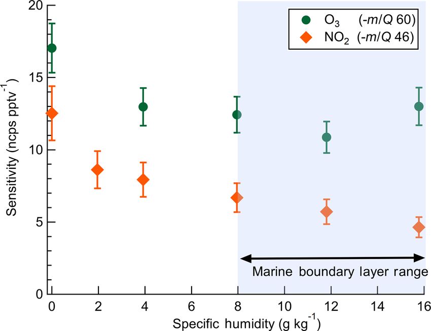
G. A. Novak et al.: Simultaneous detection of ozone and nitrogen dioxide 1893
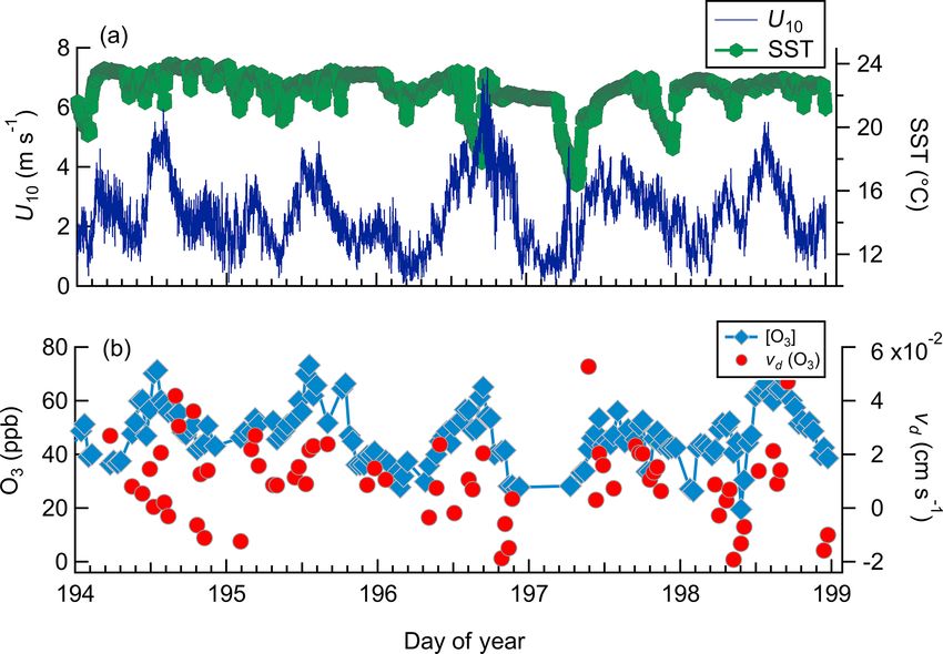
Figure 5. Normalized count rate of CO− 3 (−60 m/Q) ozone detec- Figure 6. Representative instrument backgrounding determination
tion product as a function of pressure in the IMR during sampling for O3 and NO2 , where the inlet was rapidly switched from ambient
of a constant 35 ppbv O3 source. The exponential fit of the data sampling to an overflow with dry UHP N2 indicated by the dashed
is shown by the dashed line. Fit parameters are included to allow grey line. The O3 response is fit to an exponential decay, plotted
for calculation of potential sensitivity improvements with further as solid lines, with a mean response time of 0.28 s; NO2 is fit to a
increases in IMR pressure. biexponential decay, where the initial rapid decay (τ1 ) is attributed
to gas evacuation of the inlet line and the second slower decay (τ2 )
is attributed to equilibration with the inlet walls. Best-fit estimates
used in this work. There is no evident plateauing in the sig- for τ1 of NO2 are from 0.7 to 1.2 s. τ2 for NO2 was determined to
nal increase over the IMR pressure range investigated here, be 3.2 s for this decay period.
indicating that further optimization is likely possible by op-
erating at higher IMR pressures. The increase in sensitiv-
ity with IMR pressure could be fit well with an exponen-
tial least-squares fit, which is plotted in Fig. 5. The physi- The magnitude of the O3 background was observed to vary
cal meaning of the exponential relationship is not clear. The with the O2 : N2 ratio in the reagent ion precursor flow when
source of the response of sensitivity to pressure is not defini- sampling a UHP ZA overflow with 380 ppm CO2 as shown
tive but can possibly be attributed to the increase in the to- in Fig. S2. The background O3 count rate was observed to
tal number of collisions during the 100 ms residence time increase from 3.0 × 10⁴ to 6.3 × 10⁴ ncps as the O2 volume
in the IMR and the corresponding weakening of those colli- fraction in the reagent ion delivery gas flow (fO2 ) was in-
sions. Higher collisional frequencies also lead to proportion- creased from 0.05 to 0.4. The dependence of the background
ally weaker collisions which could better preserve a weakly O3 signal on fO2 suggests that the observed background O3
bound O2 (O3 )(H2 O)− n cluster and allow for a longer lifetime
is formed directly in the alpha ion source and is not from the
in which to react with CO2 before dissociation. The opera- off-gassing of inlet and instrument surfaces. The magnitude
tional IMR pressure of 95 mbar used here was empirically se- of this background O3 does not vary when sampling UHP
lected to maximize sensitivity to O3 without increasing CDC Zero Air or N2, further confirming that the background O3 is
pressure beyond the desired range. Investigation of higher formed directly in the ion source from the O2 used to gener-
IMR pressures, up to the operation of an atmospheric pres- ate the reagent ion. An operational fO2 of 0.08 (actual volu-
sure interface, has the potential to further increase the instru- metric flow ratio O2 : N2 of 200 : 2200 sccm) was selected to
ment sensitivity to O3 . balance maximizing the total reagent ion signal while min-
imizing the O3 ion-source background (3.1 × 10⁵ cps). The
2.8 Instrument background and limits of detection magnitude of this O3 background was observed to be highly
consistent during field sampling at a constant fO2 of 0.08 and
Instrument backgrounds were assessed by periodically over- well resolved from all ambient observations (Fig. S3). The
flowing the inlet with UHP N2 during field sampling. Details 1σ deviation of the distribution of normalized adjacent dif-
of the inlet and zeroing conditions used are discussed fur- ferences of O3 signal during background periods gives an up-
ther in Sect. 3.1. During N2 overflow, O3 displayed a con- per limit of variability of 9 % between adjacent background
sistently elevated background on the order of 3.1 × 10⁵ cps periods. A variability of 9 % corresponds to a difference of
corresponding to 2.1 × 10⁴ ncps, or approximately 1.3 ppbv 70 pptv between subsequent O3 background determinations.
O3 , at a typical total reagent ion signal of 1.45 × 10⁷ cps. A The magnitude of this O3 background is a fundamental limit
representative background determination is shown in Fig. 6. on the achievable limit of detection.
www.atmos-meas-tech.net/13/1887/2020/ Atmos. Meas. Tech., 13, 1887–1907, 2020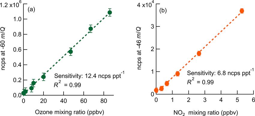
1894                                              G. A. Novak et al.: Simultaneous detection of ozone and nitrogen dioxide

   Because CO2 was not added to the UHP N2 overflow dur-          al., 2011; Veres et al., 2008). In our system we do not ob-
ing field sampling, the reaction was not driven fully to the      serve nonlinearity in the normalized O3 calibration for our
CO−                            −
    3 product and some O3 signal at −m/Q 48 was ob-               highest-concentration calibration point of 80 ppbv despite the
served during UHP N2 overflow periods as shown in Fig. S4.        CO−                                     −
                                                                      3 signal being larger than the O2 reagent ion (9 × 10
                                                                                                                                  6

The magnitude of the O3 signal observed as O−        3 was ap-
                                                                               6
                                                                  and 6 × 10 cps, respectively). The electron affinity (EA) of
proximately 55 % of the CO−     3 product  (mean  1.2 × 10⁴ and   carbonate is from 3.26 (Hunton et al., 1985) to > 3.34 eV
          3
9.6×10 ncps, respectively) during overflow periods. The to-       (Snodgrass et al., 1990) and is significantly higher than that
tal sensitivity to O3 as the sum of the O−            −
                                            3 and CO3 was ob-     of oxygen (EA 0.45 eV), making it unlikely that carbon-
served to be constant as a function of CO2 as shown in Fig. 4.    ate is involved in charge transfer reactions when excess O−    2
We therefore assigned equal sensitivity to each O3 detection      is present. At high O3 concentrations, the reagent ion sig-
product and took the sum of signal at O−                −
                                             3 and CO3 in or-     nal magnitude is reduced, which necessitates normalizing
der to determine the total background O3 concentration. This      sensitivities to the 1 × 10⁶ cps of reagent ion signal before
issue will be corrected in future deployments by the addi-        quantification. For NO2 (EA 2.27 eV), the normalized sen-
tion of CO2 to the N2 overflow used for backgrounds, which        sitivity showed no dependence on O3 concentrations from
will drive the product fully to CO− 3 . The mean background of    0 to 80 ppbv. Carbonate reagent ion chemistry has been uti-
O3 for the full field sampling period was 1.3 ± 0.3 ppbv. The     lized for detection of HNO3 and H2 O2 via adduct formation,
10 Hz precision of O3 during an individual N2 overflow pe-        raising an additional concern about potential secondary ion
riod was found to be 0.75 %, corresponding to 7.5 pptv as         chemistry (Reiner et al., 1998). In laboratory calibrations,
shown in Fig. S5. This suggests that variability in the O3        shown in Fig. S7, introduction of 0 to 40 ppb H2 O2 resulted
signal from this background source is constant over short         in the titration of the O3 signal of 0.06 ppbv per parts per
timescales and has a negligible impact on instrument preci-       billion by volume H2 O2 . H2 O2 was detected as an adduct
sion during ambient sampling.                                     with O−                −                     −
                                                                           2 and not CO3 , indicating that O2 reagent ion chem-
                                                                                                             −
   The 10 Hz limit of detection for O3 is 42 pptv for a S / N     istry is more favorable despite high CO3 signal intensity. The
of 3 and a mean background O3 signal of 2.1 × 10⁴ ncps as         Ox-CIMS O3 measurement also compared well (R 2 = 0.99)
calculated using Eq. (1), below, from Bertram et al., 2011,       against an EPA Air Quality System (AQS) O3 monitor over
where Cf is the calibration factor, [X] is the analyte mixing     1 month of ambient sampling where H2 O2 and HNO3 con-
ratio, t is averaging time in seconds, and B is the background    centrations both exceeded 5 ppbv at times (see Sect. 3.1 for
count rate. The optimum LOD from the minimum of the Al-           further discussion of field intercomparison), further support-
lan variance at an 11 s averaging time is 4.0 pptv (Fig. S6a).    ing the CO−  3 detection product as a robust indicator of O3 in
                                                                  complex sampling environments.
S      Cf [X] t
  =√                                                       (1)       Ab initio calculations of the binding enthalpies of O−  2 and
N    Cf [X] t + 2Bt                                               CO−    reagent  ions with H 2 O, HNO   3 , H  O
                                                                                                               2 2 , and CH 3 OOH
                                                                      3
The mean background signal during field sampling for NO2          were performed with the MP2/aug-cc-pVDZ-PP theory and
was 3.5 × 10³ ncps which corresponds to 0.28 ppbv. At this        basis set in order to assess the relative favorability of adduct
background level, the 10 Hz LOD for NO2 is 26 pptv for a          formation between O−             −
                                                                                         2 and CO3 . Adduct formation with O2
                                                                                                                                 −
                                                                                                 −                       −1
S / N of 3. The optimum LOD for NO2 is 2.3 pptv at an av-         was favorable relative to CO3 by 2.5 to 17 kcal mol for all
eraging time of 19 s, determined from the minimum of the          analytes that were calculated. All calculated binding enthalpy
Allan variance (Fig. S6b). The background signal of NO2 is        values are listed in Table S2.
notably above zero indicating either off-gassing from inlet
                                                                  2.10   Short- and long-term precision
walls or a secondary production of NO2 in the instrument.
A possible source of this background is from degradation of       Short-term precision of the instrument was assessed by cal-
other species such as nitric acid or alkyl nitrates on the in-    culating the normalized difference between adjacent 10 Hz
let walls. Additional calibration will be necessary to ensure     data points over a 27 min sampling period of a constant am-
that observed NO2 signal is not a secondary product of other      bient analyte concentration via Eq. (2).
species and we can currently quantify their potential interfer-
ence on measured NO2 .                                                 [mX]n − [X]n−1
                                                                  NAD = p                                                      (2)
                                                                          [X]n [X]n−1
2.9    Reagent ion saturation and secondary ion
       chemistry                                                  The standard deviation of the Gaussian fit of the distribution
                                                                  of normalized adjacent differences (NADs) is a direct mea-
During ambient sampling the ozone signal (as CO− 3 detected       sure of the short-term instrument precision (Bertram et al.,
at −60 m/Q) is of comparable magnitude to the O−  2 reagent       2011). The 1σ precision from the NAD distribution for 10 Hz
ion signal as shown in Fig. 1. High analyte concentrations        sampling of 38 ppbv ozone is 0.74 % (Fig. 7). The 10 Hz pre-
(> 5 ppbv) have been shown previously to result in nonlin-        cision for sampling of 2.3 ppbv NO2 is 1.1 % The short-term
ear calibration curves for unnormalized signals (Bertram et       precision for both analytes was larger than expected if the

Atmos. Meas. Tech., 13, 1887–1907, 2020                                             www.atmos-meas-tech.net/13/1887/2020/
G. A. Novak et al.: Simultaneous detection of ozone and nitrogen dioxide 1895
signal-to-noise ratios. This was assessed quantitatively by
calculation of the Allan variance as shown in Fig. S6 (Werle
et al., 1993).
3 Field results and discussion
3.1 Ozone field calibration and intercomparison
Performance of the Ox-CIMS was compared against a colo-
cated EPA Air Quality System (AQS) O3 monitor (Thermo
Fisher 49i, AQS ID 17-097-1007) over 1 month of ambi-
ent sampling during the Lake Michigan Ozone Study 2017
(LMOS 2017) in Zion, Illinois (Vermeuel et al., 2019). A
regression analysis between the two instruments at 1 min av-
eraging showed strong agreement (R 2 = 0.99) as shown in
Figure 7. Distribution of normalized adjacent differences measured Fig. 8. Ox-CIMS concentrations were averaged to 1 ppbv
at 10 Hz during a stable 27 min ambient sampling period of 38 ppbv
bins which was the output data resolution of the EPA data
O3 from Scripps Pier. The 1σ value of the distribution gives an
upper limit of instrument precision of 0.74 %.
logger system for the Thermo Fisher 49i. Error bars are the
1σ standard deviation of each Ox-CIMS bin average. A near
one-to-one agreement (slope of 0.99) between instruments
lends confidence to the calibration, baselining, and long-term
noise was driven by counting noise alone (10 Hz counting stability of the Ox-CIMS. The Ox-CIMS was located on the
noise limit for O3 and NO2 at the concentrations used above roof of a trailer (approx. 5 m above ground) and sampled
are 0.12 % and 0.63 %, respectively), indicating that other through a 0.7 m long, 0.925 cm i.d. PFA inlet. The inlet was
potential points of optimization in the instrument configu- pumped at a flow rate of 18–20 slpm from which the Ox-
ration are required to further improve short-term precision. CIMS subsampled at 1.5 slpm. Temperature and RH were
Notably, the observed noise source appears to be white noise recorded inline downstream of the subsampling point. The
given the Gaussian distribution of the NAD (Thornton et al., Ox-CIMS sampling point was approximately 10 m horizon-
2002b). tally from the Thermo Fisher 49i, and both instruments sam-
Short-term precision was assessed as a function of count pled at approximately equal heights. Instrument backgrounds
rate by calculating the NAD for all masses in the spectrum of the Ox-CIMS were determined every 70 min by overflow-
over a stable 27 min sampling period for both 1 and 10 Hz ing the inlet with dry UHP N2 . Calibration factors were de-
data averaging. From this assessment, precision was ob- termined by the infield continuous addition of a C-13 iso-
served to improve approximately linearly with log–log scal- topically labeled formic acid standard to the tip of the inlet.
ing for count rates between 1 × 10³ and 1 × 10⁶ cps (Fig. S8) Laboratory calibrations of the Ox-CIMS to formic acid and
as expected in the case where counting noise drives in- O3 as a function of specific humidity were determined imme-
strument precision. Above 1 × 10⁶ cps there is an apparent diately pre- and postcampaign and were used to calculate a
asymptote where precision no longer improves with count humidity-dependent sensitivity of O3 relative to formic acid.
rate. The counting-noise-limited 10 Hz precision for 106 and That relative sensitivity was then used to determine the in-
107 cps are 0.32 % and 0.1 %, respectively, while the mea- field sensitivity to O3 by scaling field sensitivities of formic
sured values were 0.75 and √ 2 %. The counting-noise-limited acid from the continuous additions. Full details of this de-
precision is calculated as N/N , where N is the number of ployment and the calibration methods are described in Ver-
counts during the integration time. This precision limit could meuel et al. (2019). The EPA O3 monitor shows a persistent
be driven by an uncharacterized source of white noise in the high bias at low O3 concentrations (< 10 ppbv) relative to the
instrument, including mass flow controller (MFC) drift, IMR Ox-CIMS. This discrepancy could arise from known interfer-
turbulence, ion optic voltage drift, and pump drift. Measure- ences from water, mercury, and other species in the 254 nm
ment precision of O3 and NO2 could be improved by a factor UV absorbance detection of ozone (Kleindienst et al., 1993).
of 5 and 2, respectively, if this noncounting noise source of
white noise was eliminated. 3.2 Eddy covariance experiment overview
In theory, detection limits can be improved by signal
averaging to a lower time resolution than the 10 Hz save The Ox-CIMS was deployed to the 330 m long Ellen Brown-
rate. Signal-to-noise ratios are expected to improve with the ing Scripps Memorial Pier (hereafter referred to as Scripps
square root of the integration time. At longer timescales, fac- Pier) at the Scripps Institution of Oceanography (32◦ 52.00 N,
tors including instrument drift become significant, creating a 117◦ 15.40 W) during July and August 2018 for EC measure-
limit on the upper end of averaging time which optimizes ments of O3 vertical fluxes. This site has been used regularly
www.atmos-meas-tech.net/13/1887/2020/ Atmos. Meas. Tech., 13, 1887–1907, 20201896 G. A. Novak et al.: Simultaneous detection of ozone and nitrogen dioxide
3.2.1 Calibration
Instrument sensitivity was assessed by the standard addi-
tion of a C-13 isotopically labeled formic acid standard for
3 min every 35 min at the ambient end of the inlet mani-
fold. Ozone mixing ratios were determined by scaling the
humidity-dependent sensitivity of O3 from pre- and postcam-
paign calibrations to the field calibrations of C-13 formic
acid. Ambient O3 was also measured at a 10 s time resolu-
tion with a 2B Technologies personal ozone monitor (POM).
The POM had a separate 10 m long, 0.47 cm i.d. PFA sam-
pling line located 12 m from the Ox-CIMS inlet manifold and
sonic anemometer. The POM was used as an independent
verification of the Ox-CIMS measurement and was not used
for calibration.
Figure 8. Regression of 1 min average O3 mixing ratios from the
3.2.2 Backgrounds and inlet residence time
Ox-CIMS against an EPA O3 monitor (Thermo Fisher 49i) binned
to 1 ppbv over 4 weeks of ambient sampling in Zion, Illinois, in
Instrument backgrounds were determined every 35 min by
May–June 2017. The solid black line is the linear least-squares re-
gression. Error bars represent the standard deviation of each bin. overflowing the entire inlet manifold with dry UHP N2 .
Instrument agreement is strong for O3 , greater than 10 ppbv, with Background and ambient count rates were first converted
an apparent bias in one or both instruments below 10 ppbv. to concentrations using the laboratory-determined humidity-
dependent sensitivities for O3 and NO2 scaled to the C-13
formic acid standard-addition sensitivity. Background con-
for EC flux observations by our group and others (Ikawa and centrations of O3 and NO2 from before and after each 30 min
Oechel, 2015; Kim et al., 2014; Porter et al., 2018). The Ox- ambient sampling period were interpolated over the ambient
CIMS was housed in a temperature-controlled trailer at the sampling period which was then subtracted from each 10 Hz
end of the pier. The Ox-CIMS sampled from a 20 m long concentration data point to obtain a background-corrected
PFA inlet manifold with the intake point colocated with a Gill time series. Background concentrations of O3 had a mean
HS-50 sonic anemometer which recorded three-dimensional 1.5 ppbv and a drift of 1 % between adjacent background pe-
winds sampling at 10 Hz. The Ox-CIMS inlet and sonic riods, determined by the distribution of the NAD of the mean
anemometer were mounted on a 6.1 m long boom that ex- background concentrations.
tended beyond the end of the pier to minimize flow distor- The signal response of O3 during dry N2 overflows were
tions. The inlet height was 13 m above the mean lower low- fit to an exponential decay function to characterize inlet gas
tide level. The Ox-CIMS inlet was located 8 cm below the response times (Ellis et al., 2010). Best-fit estimates for de-
sonic anemometer with a 0 cm horizontal displacement. The cay time constants for O3 across overflow periods were from
inlet manifold consisted of a 0.64 cm i.d. sampling line, a 0.2 to 0.44 s. NO2 decay responses were fit to a biexponen-
0.64 cm i.d. overflow line, and a 0.47 cm i.d. calibration line tial decay to characterize inlet evacuation time (τ1 ) and wall
all made of PFA. The inlet sample line was pumped at 18– interaction times (τ2 ; Ellis et al., 2010). τ2 for NO2 was de-
23 slpm (Reynolds number 3860–4940) by a dry scroll pump termined to be approximately 3.2 s. This suggests a potential
(SH-110, Agilent) to ensure a fast time response and main- interference at the NO2 peak, as NO2 is expected to have
tain turbulent flow. Flow rates in the inlet sample line were minimal wall equilibration, similar to O3 . NO2 also shows a
recorded by a mass flow meter but were not actively con- continually elevated signal during overflow periods suggest-
trolled. The inlet manifold, including calibration and over- ing off-gassing from inlet or instrument surfaces. The cause
flow lines, was held at 40 ◦ C via a single resistively coupled of this slow NO2 decay and elevated background is not clear
circuit along the length of the manifold and controlled by a but could be from degradation of nitric acid or nitrate con-
PID controller (Omega, model CNi16). The Ox-CIMS front taining aerosol on the instrument surfaces.
block and IMR were held at 35 ◦ C. The Ox-CIMS subsam- The instrument response time (τr ) for O3 can be calculated
pled 1.5 slpm from this inlet manifold through a critical ori- during zeroing periods as the time required for the signal to
fice into the IMR. Ambient humidity and temperature were fall to e−1 of its initial value. The response time of the in-
also recorded inline downstream of the subsampling point. strument was calculated for each overflow period during field
sampling, with a mean value of 0.28 s. The cutoff frequency
(fcut ) of the instrument is defined as the frequency where
√ −1
the signal is attenuated by a factor of 2 (Bariteau et al.,
2010). The cutoff frequency can also be calculated from τr
Atmos. Meas. Tech., 13, 1887–1907, 2020 www.atmos-meas-tech.net/13/1887/2020/G. A. Novak et al.: Simultaneous detection of ozone and nitrogen dioxide 1897
according to Eq. (3). 3.3 General data corrections
1 Several standard eddy covariance data filters and quality con-
fcut = (3)
2π τr trol checks were applied before analysis. General filters in-
cluded
The calculated fcut from the measured mean response time
was 0.57 Hz. This value suggests that minimal attenuation in
1. wind sector, only periods of mean onshore flow (true
the flux signal (cospectra) should be apparent at frequencies
wind direction 200–360◦ ) were used;
of less than 0.57 Hz. The instrument response time and thus
cutoff frequency are functions of the flow rate and sampling
line volume. The flow rate of 18–23 slpm was the maximum 2. friction velocity, a friction velocity (U∗ ) threshold was
achievable with the tubing and pumping configuration used applied to reject periods of low-shear-driven turbulence
here but could be improved in future to minimize tubing in- (Barr et al., 2013) described further below;
teractions and shift fcut towards higher frequencies.
3.2.3 Eddy covariance flux method 3. stationarity, each 27 min flux period was divided into
five even nonoverlapping subperiods; flux periods were
The transfer of trace gases across the air–sea interface is a rejected if any of the subperiods differed by more than
complex function of both atmospheric and oceanic processes, 40 % (Foken and Wichura, 1996).
where gas exchange is controlled by turbulence in the atmo-
spheric and water boundary layers, molecular diffusion in the The applied U∗ filter was determined by comparing the ob-
interfacial regions surrounding the air–water interface, and served U∗ values to U∗ calculated with the NOAA COARE
the solubility and chemical reactivity of the gas in the molec- bulk flux v3.6 algorithm (Fairall et al., 2011). COARE U∗
ular sublayer. The flux (F ) of trace gas across the interface was calculated using measured meteorology including wind
is described by Eq. (4), as a function of both the gas-phase speed, sea surface temperature, air temperature, and relative
(Cg ) and liquid-phase (Cl ) concentrations and the dimension- humidity. Flux periods were rejected if the observed U∗ dif-
less gas-over-liquid Henry’s law constant (H ), where Kt , the fered from the calculated U∗ by more than 50 %. The stress
total transfer velocity for the gas (with units cm s−1 ), encom- relationship of wind speed to U∗ is well understood over the
passes all of the chemical and physical processes that govern ocean. Fixed U∗ filters of ca. 0.2 m s−1 are used frequently as
air–sea gas exchange. Surface chemical reactivity terms of a default in terrestrial flux studies but would reject nearly all
the gas exchange rate are incorporated into the Kt term. observation periods in this study. The observed friction ve-
locities are consistent with other marine flux studies where
F = −Kt Cg − H Cl (4) surface roughness lengths are significantly smaller than over
terrestrial surfaces (Porter et al., 2018). Methods of deter-
Trace gas flux (F ) can be measured with the well-established mining site specific U∗ thresholds typically require long-
eddy covariance (EC) technique where flux is defined as term data series which were not available here (Papale et al.,
the time average of the instantaneous covariances from the 2006). Papale et al. (2006) applied a minimum U∗ threshold
mean of vertical wind (w) and the scalar magnitude (here of 0.1 m s−1 for forest sites and 0.01 m s−1 for short vegeta-
O3 ) shown in Eq. (5). Overbars are means, and primes are tion sites where typical U∗ values are lower. The selected U∗
the instantaneous variance from the mean. Here N is the total filter rejects an additional 44 % of the flux periods remain-
number of 10 Hz data points during the 27 min flux averaging ing after the wind direction filter. The stationarity criterion
period. rejected a further 100 flux periods, potentially driven by pe-
riods of activity on the pier driving changes in the sampled
1 XN O3 . Outliers in vd (O3 ) and the flux limit of detection were
(wi − w) O3,i − O3 = hw 0 O03 i
F= i=1
(5)
N determined and removed for points that were 3 scaled me-
F dian absolute deviations from the median. This outlier filter
vd = (6)
Cg removed an additional 16 data points. After the wind direc-
tion filter and all quality control filters were applied, 73 %
For purely depositing species where the water-side concen- of flux periods were rejected leaving 246 quality-controlled
tration is negligible, Cl and H can be neglected in Eq. (4) and flux periods. Eddy covariance flux values were calculated us-
Kt can be reformulated into a deposition velocity (vd ) calcu- ing 27 min time windows. The O3 time series was detrended
lated according to Eq. (6), where Cg is the mean gas-phase with a linear function prior to the flux calculation. The O3
mixing ratio during the flux averaging period. A summary of and vertical wind data were despiked using a mean absolute
concentration and flux results for the full deployment period deviation filter before the eddy covariance flux calculation
are given in Table 2. following Mauder et al. (2013).
www.atmos-meas-tech.net/13/1887/2020/ Atmos. Meas. Tech., 13, 1887–1907, 2020You can also read